HTDP 3.0: Software for Coping with the Coordinate Changes Associated with Crustal Motion Chris Pearson1; Robert McCaffrey2; Julie L. Elliott3; and Richard Snay4 Abstract: NOAA’s National Geodetic Survey has developed the horizontal time-dependent positioning 共HTDP兲 software to provide a way for its users to estimate the coordinate changes associated with horizontal crustal motion in the United States. HTDP contains a model for estimating horizontal crustal velocities and separate models for estimating the displacements associated with 29 earthquakes 共two in Alaska and 27 in California兲. This software is updated periodically to provide more accurate estimates for crustal velocities and earthquake displacements, as well as to include models for additional earthquakes. In June 2008, NGS released version 3.0 of HTDP 共HTDP 3.0兲 that introduces an improved capability for predicting crustal velocities, based on a tectonic block model of the western contiguous United States 共CONUS兲, that is, from the Rockies to the Pacific coast. Values for the model parameters that predict the velocity at any point within the domain were estimated from 4,890 horizontal velocity vectors 共derived from repeated geodetic observations兲, 170 fault slip rates, and 258 fault slip vector azimuths. Extensive testing indicates that this model can predict velocities within CONUS with a standard error of less than 2 mm/year in both the north and east components. HTDP 3.0 also introduces a model for the combined coseismic and postseismic displacements associated with the magnitude 7.9 Denali earthquake that occurred in central Alaska on November 3, 2002. DOI: 10.1061/共ASCE兲SU.1943-5428.0000013 CE Database subject headings: Datums; Computer software; Geodetic surveys. Author keywords: Datums.
Introduction In 1992, NOAA’s National Geodetic Survey 共NGS兲 introduced the first version of the horizontal time-dependent positioning 共HTDP兲 software for providing the geospatial community a way to estimate changes in horizontal positional coordinates associated with crustal motion 关www.ngs.noaa.gov/TOOLS/Htdp/ Htdp.shtml; see also Snay 共1999, 2003兲兴. In particular, the HTDP software contains models for horizontal crustal velocities in the United States. This software also contains models that predict the horizontal displacements associated with several major U.S. earthquakes. NGS has since released new versions of HTDP with revised models on several occasions to improve the accuracy of the estimated velocities and to include models for additional earthquakes. In June 2008, NGS released version 3.0 of HTDP 共HTDP 3.0兲 1 Illinois State Geodetic Advisor, National Geodetic Survey, 2300 South Dirksen Pkwy., Springfield, IL 62703 共corresponding author兲. E-mail:
[email protected] 2 Principal, Troy Geophysics, Troy, NY 12180. E-mail: mccafr@ rpi.edu 3 Ph.D. Student, Geophysical Institute, Univ. of Alaska Fairbanks, Fairbanks, AK. E-mail:
[email protected] 4 Chief Spatial Reference System Division, National Geodetic Survey, 1315 East West Highway, Silver Spring, MD 20910. E-mail: richard.
[email protected] Note. This manuscript was submitted on October 17, 2008; approved on July 1, 2009; published online on July 3, 2009. Discussion period open until October 1, 2010; separate discussions must be submitted for individual papers. This paper is part of the Journal of Surveying Engineering, Vol. 136, No. 2, May 1, 2010. ©ASCE, ISSN 0733-9453/2010/2-80– 90/$25.00.
which incorporates the newest model for predicting horizontal crustal velocities in the western part of the contiguous United States 共CONUS兲. HTDP 3.0 also introduces a model for predicting the displacements associated with the magnitude 7.9 Denali earthquake, which devastated central Alaska on November 3, 2002. This paper describes these new models, plus it addresses other recent revisions to the HTDP software. Estimating the horizontal surface velocity for a user-specified location is one of two primary functions supported by HTDP. The software’s second primary function is to predict horizontal displacements for a user-specified location and a user-specified period of time. For this second function, HTDP multiplies the predicted velocity by the time difference and then adds any earthquake-related displacements that occurred during the specified time period. In predicting velocities and/or displacements, HTDP applies numerical models for horizontal crustal motion which have been derived from repeated geodetic observations, as well as from geological, seismological, and other geophysical information. The reality of crustal motion implies that positional coordinates in many locations change as a function of time. Hence, it is inappropriate to specify positional coordinates for these locations without also specifying the date to which these coordinates correspond. Let us call this date the reference date for the given coordinates. People may apply HTDP to update 共or backdate兲 the positional coordinates of a point from one reference date to corresponding coordinates for another reference date. This software simply adds 共or subtracts兲 the point’s predicted displacement between the two dates to the positional coordinates of the starting reference date. HTDP also enables its users to update 共or backdate兲 certain types of geodetic observations 关differential global positioning sys-
80 / JOURNAL OF SURVEYING ENGINEERING © ASCE / MAY 2010
Downloaded 04 Jun 2010 to 128.113.82.223. Redistribution subject to ASCE license or copyright. Visithttp://www.ascelibrary.org
tem 共GPS兲, distances, azimuths, horizontal angles, horizontal directions兴 from the value that was measured on the day of observation to the value that would have been measured on some other date. Indeed, as part of the NSRS2007 readjustment of NAD 83, NGS updated all pertinent GPS observations that were observed in California between 1986 and 2005 to corresponding values that would have been observed on January 1, 2007. NGS then performed a simultaneous 共fixed-Earth兲 adjustment of these updated observations to determine the NAD 83 共NSRS2007兲 positional coordinates for over 1,000 reference stations that provide geodetic control for California 共Pearson 2005兲. The need to update observations to a common date, called data homogenization, is a burden of living in earthquake country; but this need is not unique to California. HTDP 3.0 predicts velocities primarily relative to the International Terrestrial Reference Frame of 2005 共ITRF2005兲 共Altamimi et al. 2007兲, but it is able to convert these predicted values to equivalent values in other popular reference frames, including all other realizations of ITRF, all realizations of the World Geodetic System of 1984 共WGS84兲, and to the CORS96 realization of the North American Datum of 1983 关NAD 83 共CORS96兲兴. Consequently, HTDP 3.0 may be used to transform positional coordinates and/or velocities from one reference frame to another in a manner that rigorously accounts for the relative motion between these frames. The NGS-adopted transformation equations between ITRF2005 and NAD 83 共CORS96兲 are given in the Appendix of this paper.
Nature of Crustal Motion Since the 1960s geologists have known that the Earth’s surface is partitioned into a number of tectonic plates that are in constant motion relative to each other at rates which are typically about several centimeters per year. These plates generally move as rigid blocks; however, at their edges there is a zone 共often called a plate boundary兲 where they rub against each other and deform, causing earthquakes and other geophysical phenomena. CONUS straddles the boundary between the North American plate and the Pacific plate within the part of California located south of Mendocino, California. In the northwest corner of CONUS, the North American plate is colliding with the oceanic Juan de Fuca plate and its smaller neighbors: the Gorda and Explorer plates. Moreover, the Pacific coast of Alaska resides in the deformation zone associated with the boundary between the North American plate and the Pacific plate. As a result, most of California, Nevada, Oregon, Washington and Alaska are undergoing crustal deformation. Like other continental plate boundaries, the deformation extends hundreds of kilometers to either side of the boundary proper. As such, the deformation in CONUS extends eastward, though at a lower rate, as far as Salt Lake City, Yellowstone, and the Rio Grande Rift. In the ITRF and WGS84 reference frames, all points on both the Pacific and North American plates have nonzero velocities reflecting the movement of the plates 共Snay and Soler 2000兲. The NAD 83 reference frame, however, is defined so that all points on the North American plate, located sufficiently far from the plate boundary zone, will have 共on average兲 zero horizontal velocities. Points located within the Pacific-North American plate boundary zone will have NAD 83 velocities that are transitional between the respective velocities of these two plates and as a result have nonzero NAD 83 velocities with magnitudes of up to 5 cm/yr, the Pacific plate velocity.
The deformation modeled by HTDP is largely caused by the tectonic plates that interact within the western margin of North America. Much of the motion is assumed to be accommodated by geologic faults that extend from Earth’s surface to points deep within Earth’s crust. The crust, however, is comprised of two layers that deform in quite different ways. These layers are separated by a broad zone called the brittle-ductile transition zone. In the top layer 共known as the brittle region兲 rocks deform following the same elastic principles as ordinary engineering materials. Here, deformation causes increasing stress that eventually exceeds the frictional strength of the faults leading to an earthquake. Deeper in the crust, where conditions are hotter, the rocks behave in a ductile manner. Here deformation occurs by a slow continuous process and stress never reaches a value sufficient to cause catastrophic failure. As a result, two quite different processes are responsible for the deformation in the western states. The first of these is slow response of the deeper part of the crust and the elastic response of the upper crust to the differential movement of the tectonic plates. It is assumed that faults in the lower crust accommodate this motion by slipping without earthquakes and this deformation is transmitted through the elastic crust to the surface and causes the secular velocity field. While the resulting secular velocities are fairly small, up to about 5 cm/year in some places, the effect on the positions of surface points accumulates with time and is large enough that it cannot be ignored. The secular velocities are assumed to be relatively constant, so that once this part of the field is mapped, it need not be changed, although periodic updates are needed to reflect our improved knowledge of it. The second part is the displacement caused by earthquakes that result when elastic stress associated with the secular velocity field accumulates along a fault. At some instant, the force caused by the stress acting on the fault exceeds the frictional force which keeps the fault locked. In this case, a fault will suddenly slip and quite large displacements can happen within a period of a few minutes or less. This so-called coseismic portion of the deformation field is therefore different because earthquakes happen in unpredictable ways. So each time there is a new earthquake, the HTDP software must be updated with the appropriate parameters for modeling the deformation. Because these two processes are very different both temporally and spatially, two quite different methodologies are required to model them. The secular velocity field is represented by a two-dimensional grid-interpolation scheme of the velocity field that provides an estimate of the velocity of any point located within the plate boundary zone, while earthquakes are represented using dislocation models 共Okada 1985; Savage 1980兲 that define the slip on related geologic faults.
Earthquakes The deformation associated with an earthquake is caused by a fault in the Earth that slips suddenly due to the stress in the surrounding rocks. Sometimes the break extends to the surface in which case the displacement will change very suddenly as one side of the fault will move one way while the opposite side moves in the opposite direction. Often, however, the break does not reach the surface. Even in this case, the earthquake will cause surface displacements because slip on the fault will cause sympathetic movement in the surrounding rocks and this deformation will propagate through the Earth to the surface. Slip on the fault, with its accompanying decrease in stress on the fault, allows the elastic material surrounding the fault to rebound as the elastic JOURNAL OF SURVEYING ENGINEERING © ASCE / MAY 2010 / 81
Downloaded 04 Jun 2010 to 128.113.82.223. Redistribution subject to ASCE license or copyright. Visithttp://www.ascelibrary.org
Table 1. List of Earthquakes Having Models in HTDP 3.0
Fig. 1. Time series of coordinates for the CORS site, FAIR, for the period spanning the Denali earthquake. The time axis starts on December 2, 2001, or the first day when ITRF00 became operational. Major division correspond to 1 year of data while the minor ticks represent 30 days. The Denali earthquake occurred near the end of the first year of the time interval. The plots show both a sudden coseismic displacement and a more gradual exponential decay associated with postseismic slip. Arrows show the coseismic displacement associated with the Denali Earthquake as estimated with HTDP 3.0. These arrows can be compared with the step change in the north and east time series at the time of the earthquake.
strain in the surrounding rocks 共caused by deformation associated with the secular velocity field兲 is released. This release in the elastic strain in the rocks surrounding the earthquake rupture results in deformation associated with the earthquakes extending a considerable distance from the fault. In large earthquakes, measurable coseismic displacement can extend hundreds of kilometers from the fault. In small, shallow earthquakes, where the material near the fault is cool enough to be fully elastic, the deformation associated with the earthquake will be complete within a few minutes and coseismic deformation is all that will occur. However in larger or deeper earthquakes, the rupture may extend deep enough so that the bottom of the active part of the fault is near the brittle-ductile transition. The adjacent ductile parts of the crust will respond to the stress change caused by the earthquake in a viscous manner and the resulting deformation may last for several months or years. This slow deformation does not cause noticeable seismic waves or shaking and is called postseismic deformation 共Freed 2005, 2007兲. Postseismic slip is important to surveyors because it contributes to the total deformation field on the surface that will affect the relative position of points causing them to change from the relationships measured during earlier surveys. HTDP currently includes no mechanism for realistically modeling postseismic motion because the effect is usually small compared to coseismic deformation and geophysical models that can be used to calculate its effect are rare. The final deformation field associated with the earthquake is the sum of the coseismic and postseismic components. Fig. 1 shows the coseismic 共especially noticeable as the step function in the north coordinate兲 and postseismic 共the long asymptotic tail following the step function兲 deformation as revealed by time series of positional coordinates for the continuously operating reference station 共CORS兲 known as FAIR for a time period including the 2002 Denali earthquake. This earthquake is the largest that occurred within the United States since the CORS network was established. HTDP 3.0 contains models for 29 earthquakes 共see Table 1兲 which have been developed from measured deformation on the Earth’s surface. Locations range from Alaska to the Mexican border, although all but two are located in California. At this
Earthquake
Date
Magnitude
Number of dislocations
Parkfield, Calif. El Centro, Calif. Red Mountain, Calif. San Jacinto, Calif. Kern County, Calif. San Jacinto, Calif. Prince Wm. Sound, Alaska Parkfield, Calif. Borrego Mtn, Calif. San Fernando, Calif. Imperial Valley, Calif. Coyote Lake, Calif. Homestead Valley, Calif. Coalinga, Calif. Morgan Hill, Calif. Kettleman Hills, Calif. Chalfant Valley, Calif. North Palm Springs, Calif. Superstition Hill, Calif. Whittier Narrows, Calif. Loma Prieta, Calif. Petrolia, Calif. Landers/Big Bear, Calif. Joshua Tree, Calif. Northridge, Calif. Hector Mine, Calif. San Simeon, Calif. Parkfield, Calif. Denali, Alaska
1934 1940 1941 1942 1952 1954 1964 1966 1968 1971 1979 1979 1979 1983 1984 1985 1986 1986 1987 1987 1989 1992 1992 1992 1994 1999 2003 2004 2002
6.0 6.7 5.9 6.5 7.7 6.2 9.2 5.6 6.4 6.4 6.6 5.9 5.6 6.5 6.2 6.1 6.5 6.0 6.6 6.0 7.1 7.1 7.3 6.1 6.6 7.1 6.5 6.0 7.9
98 5 1 1 3 1 68 98 1 4 1 1 1 1 1 1 2 1 2 1 1 1 26 19 1 75 200 300 911
time, only the coseismic deformations associated with the earthquakes listed in Table 1 are modeled in HTDP. There are two other earthquakes with magnitudes greater than 6.2 that occurred in CONUS since 1980 that are not included in HTDP. These are the M 7.3 Borah Peak, Idaho earthquake which occurred in 1983 and the M 6.7 Nisqually, Washington earthquake which occurred in 2001. We do not intend to include a model of the 1983 Borah Peak earthquake because it predates the era of GPS surveys and NGS has decided to discontinue support for including classical surveys in future readjustments 共Pearson 2005兲. We hope to include a model of the 2001 M 6.7 Nisqually, Washington earthquake in a future version of HTDP. Another 共third兲 type of slow, time-dependent motion that has been observed in the western U.S. is called a slow-slip event. These events produce surface displacements that appear very much like earthquakes but occur over weeks rather than seconds. They are similar to postseismic motions in that they do not produce seismic shaking but differ in that they are isolated in time rather than following a seismic event. Unlike secular velocities they are limited in duration. Such slow slip events have been observed along the coastal regions of Oregon and Washington 共Dragert et al. 2004; Szeliga et al. 2008兲 and along the San Andreas fault in central California 共Linde et al. 1996兲. Since the surface displacements observed to date from these events have been small 共⬍5 mm兲, they are not specifically modeled in HTDP 3.0.
82 / JOURNAL OF SURVEYING ENGINEERING © ASCE / MAY 2010
Downloaded 04 Jun 2010 to 128.113.82.223. Redistribution subject to ASCE license or copyright. Visithttp://www.ascelibrary.org
Fig. 2. Schematic diagram of a dislocation. The rectangle represents the dislocation surface or slipping patch on a fault. The deformation measured on the surface depends on the strike 共␣兲 and dip 共␦兲 of the fault plane, the length of the dislocation 共L兲, the depth to the top 共d兲 and bottom 共D兲 surface of the dislocation measured along the fault plane and the latitude and longitude 共 and 兲 of the fault center.
Dislocation Models Predicting the effect of an earthquake on positional coordinates utilizes the relatively simple mathematical equations provided by dislocation theory 共Okada 1985; Savage 1980兲. The equations predict the elastic response of a uniform elastic half-space to slip on a rectangular patch embedded within the half-space. Each dislocation represents a rectangular patch 共fault surface兲 in the Earth where one side slips relative to the other in the plane by a uniform amount. The name, dislocation, is used because the slip displacement is uniform over the rectangle thereby producing a discontinuity along the edges of the patch. The model is shown conceptually in Fig. 2. A dislocation model is thought to be similar to what happens during an earthquake where one side of the fault slips relative to the other. While a single dislocation can be used to model an earthquake, real earthquakes are much more complex. This oversimplification can be overcome by partitioning the fault into a series of smaller rectangular dislocations which, taken together, may better approximate the complexity associated with a real earthquake. In the Denali earthquake discussed below, for example, over 900 dislocations were used to map the fault plane. The dislocations used in HTDP 3.0 were determined by varying the properties of the dislocations, such as the amount of slip and the geometry of the rectangular patches, until the predictions of the dislocation model provides a satisfactory match with observations made before and after the earthquake. The two main types of observations used to constrain dislocation models are surface measurements of displacements measured with GPS data and, sometimes, InSAR 共Interferometric Synthetic Aperture Radar兲 data 共Bürgmann et al. 2000兲.
Updated Model of the Secular Velocity Field The updated model of the secular field started with an analytical model representing horizontal crustal motion developed using the computer code DEFNODE 共McCaffrey 1995, 2002兲 which incorporates all major active faults located in western CONUS in a single model developed by combining studies by McCaffrey 共2005兲 of the Pacific northwest and McCaffrey et al. 共2007兲 of the southwestern United States. The blocks included in the model are shown in Fig. 3.
Fig. 3. 共Color兲 Tectonic blocks used to model secular motion. Lines outline the boundaries of the tectonic blocks used to model the data. The ITRF2005 velocity measurements and geological data used to constrain the secular velocity model incorporated into HTDP 3.0 are also shown.
The predicted velocity field is based on rotating, fault-bounded crustal blocks 共spherical caps兲 subject to elastic and anelastic strain rates. Rotations of the blocks are described by angular velocities, sometimes called Euler poles. The angular velocity is constrained to have the center of the Earth as its origin, forcing the plates to move tangentially to the surface. Hence the plates have only east and north velocities due to rotations. Elastic strain rates arise where the edges of the blocks 共the faults兲 come into contact at a frictional surface. As the blocks slide past one another, frictional forces cause the shallow parts of the faults to remain stuck and this induces strain in the blocks adjacent to the fault. The amount of strain is estimated from the relative velocities of the blocks across the fault and the degree of locking 共that varies from zero to one where zero corresponds to free slip and one corresponds to a fully locked fault兲. These parameters are passed through a dislocation model 共as described earlier兲 but in a “back-slip” mode, or negative earthquakes, described by Savage 共1983兲. The linear combination of the rotational motions and the back-slip velocities gives the appearance of the motion about a locked fault. The model also allows the blocks to deform under horizontal, uniform strain rates. This allows for the distributed deformation associated with minor, unmodeled faults within the blocks that are often found in tectonically active areas. The uniform strain rates are implemented using the spherical-coordinate strain tensor of Savage et al. 共2001兲. We used this model to invert or solve for parameters that control the surface velocities. In the inversion, the free parameters are related to the blocks, the faults, and the GPS velocity fields. Each block has three free parameters describing the x, y, and z components of its angular velocity and three describing the EE, NN, and EN components of its uniform strain rate tensor. The parameterization of locking on the faults is through a parameter which is defined as one minus the free slip fraction. Hence, = 1 represents JOURNAL OF SURVEYING ENGINEERING © ASCE / MAY 2010 / 83
Downloaded 04 Jun 2010 to 128.113.82.223. Redistribution subject to ASCE license or copyright. Visithttp://www.ascelibrary.org
Table 2. Geodetically Derived Velocity Vectors Used to Constrain the Secular Velocity Model in HTDP 3.0 Code ITR5 SNRF
Number Number Weight Sig min Sig max WRMS Sum used total factor 共mm/year兲 共mm/year兲 NRMS 共mm/year兲 of weights 55 18
290 22
0.44 1.00
0.5 0.3
3.0 3.0
1.23 1.12
0.66 0.43
377 246
DXB2 HT04 HT05 WILL CEA1 CMM4
16 67 94 36 1,285 1,195
16 67 110 71 1,403 1,318
1.00 1.00 1.00 0.25 1.00 1.00
0.3 0.5 0.5 0.5 0.3 0.3
5.0 3.0 3.0 3.0 2.5 2.5
0.67 0.90 0.87 1.19 1.21 1.15
0.85 0.86 1.01 1.14 1.33 1.22
20 146 139 78 2,150 2,130
DMEX PBO7 PNW7
12 437 578
14 795 670
0.44 0.25 1.00
0.5 0.4 0.3
3.0 3.0 2.5
0.75 1.07 1.16
1.07 0.95 0.58
12 1,100 4,590
full locking on the fault 共no slip at the boundary兲 and = 0 represents a free slip boundary at the fault. For short faults, a single value of is used along its entire length while longer faults may have changing along strike. The amount of back-slip applied at a point along the fault is −V where V is the slip vector locally on the fault. Finally, the GPS-derived velocities used to constrain the model parameters come from several individual publications, where the set of velocities from one publication may be referred to a different reference frame than the set from another publication. Hence, each set of vectors was transformed into ITRF2005 by applying three rotation parameters whose values were estimated along with the other parameters involved in our model. This estimation problem is highly nonlinear and was solved iteratively by the downhill simplex method. The general geometry of the model has been described by McCaffrey 共2005兲 for the southern part of the North AmericanPacific plate boundary and McCaffrey et al. 共2007兲 for the northern part. In this work, the two models were merged by modifying the block geometries at their common boundary along the latitude of the northern California border. Blocks included in the inversion process are shown in Fig. 3. The model is constrained by the following data: 4,890 horizontal velocity vectors 共derived from repeated geodetic observations—mostly GPS observations兲, 170 fault slip rates from geologic studies, and 258 fault slip vectors taken from earthquakes and geologic studies. The distribution of geodetically derived velocity measurements are shown in Fig. 3 and details of the various geodetic data sets are summarized in Table 2. Note that only horizontal velocities were used in the inversion. Using these data, the model parameters were adjusted iteratively to produce an improved match to the weighted data. The fitness criterion was the reduced chi-square statistic; in the end this was 1.38 indicating that the data are fit at about their level of uncertainty. In Table 2, the normalized RMS 共NRMS兲 indicates the degree of fit to the particular velocity field; a value of around unity indicates an acceptable fit. The weighted RMS 共WRMS兲 is a measure of the weighted average residual for that field; for the majority these are about 1 mm/year or less. Note that the data sets contained in Table 2 may have originally been expressed in various reference frames. Hence, as part of the DEFNODE process, the ITR5 velocity field was selected to define the reference frame and the velocity vectors contained in each of the other data sets were transformed into that frame. We
Data source Altamimi et al. 共2007兲 Stable North American Reference Frame Working Group 共2007兲 Dixon et al. 共2002兲 Hammond and Thatcher 共2004兲 Hammond and Thatcher 共2005兲 Williams et al. 共2006兲 California Earthquake Authority Z. K. Shen et al. 共“A unified analysis of crustal motion in California 1970–2004,” The SCES Crustal Motion Map, unpublished, 2007兲 Márquez-Azúa and DeMets 共2003兲 PBO 4/2007 McCaffrey et al. 共2007兲; Payne et al. 共2007兲
selected the data set called ITR5, because its vectors are expressed in the rigorously defined ITRF2005 frame 共Altamimi et al. 2007兲. Consequently, HTDP 3.0 predicts velocities relative to ITRF2005, but the software is able to convert these predicted ITRF2005 velocities to other popular reference frames, including NAD 83 共CORS96兲. Fig. 4 displays predicted secular velocities in western CONUS relative to NAD 83 共CORS96兲. Once model parameters have been estimated with DEFNODE, these parameters can be used to predict the horizontal velocity at any point in western CONUS by running DEFNODE in its predictive 共forward model兲 mode. HTDP uses four grid files to interpolate the secular velocities predicted by DEFNODE. These grids cover different regions with different cell sizes in order to maintain a desired level of accuracy in regions of higher velocity gra-
Fig. 4. 共Color兲 Horizontal velocities in western CONUS relative to NAD 83 共CORS96兲 as predicted with HTDP 3.0. Colors indicate velocity magnitudes and arrows indicate velocity directions.
84 / JOURNAL OF SURVEYING ENGINEERING © ASCE / MAY 2010
Downloaded 04 Jun 2010 to 128.113.82.223. Redistribution subject to ASCE license or copyright. Visithttp://www.ascelibrary.org
Table 3. Interpolation Grids Incorporated into HTDP 3.0 Longitude range 125° 125° 125° 121°
to to to to
100° W 122° W 119° W 114° W
Latitude range
Cell spacing 共min兲
Grid dimensions
Region
31° – 49° N 40° – 49° N 36° – 40° N 31° – 36° N
15 3.75 3.75 3.75
101⫻ 73 49⫻ 145 97⫻ 65 113⫻ 81
Entire region Pacific NW Northern California Southern California
“Observed” velocity vectors for seven small regions were excluded from the inversion because these regions contain geophysical features such as volcanoes or the epicentral region of large recent earthquakes where the deformation is not easily modeled using the methodology described above. These regions are described by the coordinates 共latitude and longitude兲 of the region’s center and a radius. The regions are listed in Table 4 below. Users should be aware of these regions because the predicted velocities and thus the corrections applied to positions and survey measurements may be less accurate there than elsewhere in the study area.
dients. HTDP will automatically choose the most accurate grid for the point in question. The grids are summarized in Table 3. Note that HTDP is now capable of estimating secular velocities over the region from 31° to 49° N latitude and from 125° to 100° W longitude, which is significantly larger than the previous version which extended from 31.75° to 50° N latitude and from 125° to 111° W longitude. For a point located on that part of the North American plate which resides external to the interpolation grids 共presumably “stable” North America兲, HTDP 3.0 uses the Euler pole for North America, which was derived by Altamimi et al. 共2007兲, to predict the point’s ITRF2005 velocity. It should be noted that when the ITRF2005 velocity for such a point is transformed to its corresponding NAD 83 共CORS96兲 velocity, then the resulting velocity usually differs from zero. Hence, HTDP 3.0 predicts small but nonzero NAD 83 horizontal and vertical velocities for points located in stable North America for two reasons, both related to deficiencies in the definition of NAD83: first, because the velocity-related parameters included in the transformation from ITRF96 are based on the NUVEL1A-NNR plate motion model 共DeMets et al. 1990, 1994兲 rather than the plate motion model associated with ITRF2005; and second, because the ITRF2005 reference frame is moving relative to the ITRF96 reference frame. To rectify this problem, NGS is considering the possibility of introducing a more modern realization of NAD 83 within the next few years, after the next ITRF realization is released. This modern NAD 83 realization would be directly linked to this next ITRF realization rather than indirectly linked to it via a relationship with ITRF96. The new relationship between NAD 83 and ITRF would also be based on the prevailing plate motion model existing at the time when the new NAD 83 realization is formulated. That is, the new relationship between NAD 83 and ITRF would be based on the prevailing estimates for the parameters that quantify the Euler Pole for the North American plate relative to the new ITRF realization. Note that the same datum transformation can cause HTDP to predict small vertical velocities in the NAD83 reference frame when interpolating from our velocity grids even though the gridded velocities, which are in ITRF2005, have zero vertical velocities. This affects only HTDP3.0. In previous versions 共HTDP2.9 and earlier兲 velocities for the grid nodes are referred to NAD 83 共CORS96兲.
Validation of Secular Field The predicted secular velocity field contained in HTDP 3.0 was tested by comparing it to two GPS-derived data sets. The first data set was the GPS vectors used to develop the model. Here we were simply checking to see that the grids in HTDP accurately represent the velocity field. The agreement 共summarized in Table 5兲 was generally very good. The RMS residuals for 4,890 vectors were 0.75 mm/year in the north component and 0.68 mm/year in the east component. The maximum residuals were a little over 10 mm/year in both the north and east components; however the 13 residuals with a combined vector greater than 5 mm/year fall within a narrow linear concentration that seems to follow the San Andreas Fault system through California with about half distributed along the creeping segment of the San Andreas Fault 共Thatcher et al. 1997兲. A poor fit in this area is not unexpected because the interpolation procedure used by HTDP cannot be expected to follow the very high strain gradients associated with the creeping fault. Histograms of the residuals are shown in Figs. 5共a and b兲. The second test data set used to validate the secular field for HTDP 3.0 was the velocities estimated by the California Spatial Reference Center using the “Scripps Epoch Coordinate Tool and Online Resource” 共SECTOR兲 共Nikolaides 2002兲. The velocities we used are available at: http://sopac.ucsd.edu/cgi-bin/ rerunTimeSeries.cgi. While some of the stations in this data set are also used to develop the model, the data were independently processed and the SECTOR utility for determining the velocities
Table 4. Circular Regions Excluded from the Inversion Center latitude Name Mammoth lakes volcanic region Coso volcanic field Yellowstone volcanic region South sister volcano Mount St. Helens volcano Landers quake Landers quake
Center longitude
Degrees
Minutes
Seconds
Degrees
Minutes
Seconds
Radius 共km兲
37 36 44 44 46 34 34
42 0 25 6 12 24 0
0 0 48 0 0 ⫺0 0
118 117 110 121 122 116 116
54 45 40 51 10 30 30
0 0 12 0 48 0 0
20 20 50 20 20 20 20
JOURNAL OF SURVEYING ENGINEERING © ASCE / MAY 2010 / 85
Downloaded 04 Jun 2010 to 128.113.82.223. Redistribution subject to ASCE license or copyright. Visithttp://www.ascelibrary.org
Table 5. Summary of Data Sets Used to Test HTDP 3.0
Data set Inversion data Sector in HTDP30 Sector in HTDP29
RMS north residual 共mm/year兲
RMS east residual 共mm/year兲
Number of vectors
0.75 1.9 3.3
0.68 1.7 3.1
4558 630 630
is very different from the method used by the inversion. In addition, they included up to two years of additional measurements. For these reasons it is believed that velocity estimates for the common stations are independent. Initially the comparison produced a large number of outliers, however, most of these proved to be cases with short time series and these disappeared once test data sets were restricted to stations with a minimum of 2 years of data. The fit of these data was excellent 共see Table 5兲 with the RMS residuals being 1.9 mm/year for the north and 1.7 mm/year for the east components. Over 90% of the stations had a combined residual of less than 3 mm/year. Histograms of the residuals are shown in Figs. 6共a and b兲 and a map of points with total residuals greater than 5 mm/year is shown in Fig. 7. By way of comparison, using the same data set, HTDP 2.9 has RMS residuals of 3.3 mm/year for the north and 3.1 mm/year for the east component. So introducing the new model of the secular field produces a
Fig. 6. 共a兲 Histogram of N component residuals for SECTOR derived velocities; 共b兲 histogram of east component residuals for SECTOR derived velocities
Fig. 5. 共a兲 Histogram of north component residuals of GPS vectors included in inversion; 共b兲 histogram of east component residuals
Fig. 7. Map showing location of sector test points with velocity residuals exceeding 5 mm/year in magnitude
86 / JOURNAL OF SURVEYING ENGINEERING © ASCE / MAY 2010
Downloaded 04 Jun 2010 to 128.113.82.223. Redistribution subject to ASCE license or copyright. Visithttp://www.ascelibrary.org
Fig. 8. Predicted displacement for the Denali earthquake. Contours show the magnitude of the displacements 共without regard for the opposite direction of the displacement on different sides of the fault兲 and arrows show predicted directions of the displacements.
significant 共over 30%兲 improvement in the fit to the observed velocities from the SECTOR utility.
Denali Earthquake The Denali earthquake occurred on Sunday, November 3, 2002 at 22:12 UTC in south central Alaska about 283 km NNE of Anchorage. The earthquake had a magnitude 共Mw兲 of 7.9 and was the strongest ever recorded in the interior of Alaska and one of the largest earthquakes recorded within the United States 共EberhartPhillips et al. 2003兲. The earthquake produced displacements of several meters near the fault and measurable displacements throughout most of central Alaska. Because this earthquake was primarily a strike-slip event where the rupture plane extended to the surface, points on opposite sides of the fault will move in opposite directions producing a very large relative displacement for a pair of points that happen to be located on opposite sides of the fault. The earthquake was predominantly a right-lateral strikeslip event; however, it started with a thrust subevent on the previously unrecognized Susitna Glacier fault. The dislocation model we used for this earthquake was developed by Elliott et al. 共2007兲, which was constrained by surface deformation measurements 共both GPS data and range offsets derived from a synthetic aper-
ture radar 共SAR兲 amplitude image兲 without using seismic body waves. Because of the complexity of this event, combined with the fact that the rupture extended over 250 km along the Denali fault, the dislocation model used to model this earthquake, with 910 elements, was the most complex ever incorporated in HTDP. Indeed the number of dislocation elements in this model is more than three times any of the other dislocation models included in the software. The predicted displacements for the Denali earthquake are shown in Fig. 8. The predicted movement associated with the Denali earthquake was tested using a set of over 200 GPS-derived displacement vectors. The agreement between predicted and observed displacements was reasonably good with an RMS misfit of 0.1 m in both the north and east components. A few quite large discrepancies 共sometimes ⬎1 m兲 were found in the vicinity of the fault trace. This probably indicates that complex fault geometry can introduce significant errors in the predicted deformation for points located near the rupture plane. This is particularly true for large earthquakes that rupture the Earth’s surface. As a result, care must be used when correcting surveys for earthquakes when the survey area crosses a fault rupture that extends to the Earth’s surface. As shown in Fig. 1 we also compared the HTDP 3.0 predicted displacement for this earthquake for the CORS station FAIR with the time series from this station covering the time of the earthquake. JOURNAL OF SURVEYING ENGINEERING © ASCE / MAY 2010 / 87
Downloaded 04 Jun 2010 to 128.113.82.223. Redistribution subject to ASCE license or copyright. Visithttp://www.ascelibrary.org
Future Plans The major deficiency with HTDP 3.0 is the lack of a detailed crustal motion models for Alaska. Currently the HTDP 3.0 model includes models for only the Prince William Sound earthquake of 1964 and the Denali earthquake of 2002, and the model for the secular velocity field has not been updated. Over the next year or so, HTDP may be revised to include a model of recent major 共greater than magnitude 7兲 earthquakes and an improved model for Alaska’s secular velocity field.
Conclusions The HTDP software has been updated to include a new model of the secular velocity field in western CONUS and a model of the Denali earthquake of 2002. The model was released in June 2008 replacing the previous version, HTDP 2.9 共Pearson and Snay 2007兲, which had been used in the recently completed NSRS2007 readjustment 共Pearson 2005兲. HTDP 3.0 is applied in all OPUS solutions to convert computed NAD 83 coordinates from the day when the submitted GPS data was observed to a common reference date of January 1, 2002. The HTDP 3.0 software is also available for download at http://www.ngs.noaa.gov/PC_PROD/ HTDP/. Finally, the latest version of HTDP can be run interactively on the Web at http://www.ngs.noaa.gov/TOOLS/Htdp/ Htdp.shtml. With its new secular velocity field model, HTDP is now capable of predicting secular velocities over the region from 31° to 49° N latitude and from 125° to 100° W longitude. This is significantly larger than the region covered by the previous version of HTDP. The model also includes three subgrids with reduced cell spacing that allows HTDP to obtain higher accuracy in regions of higher velocity gradients in the tectonically active areas of California and the Pacific Northwest. A test of the secular field model versus an extensive data set compiled by the California Spatial Reference Center showed that the new model of the secular velocity field produces a significant 共over 30%兲 improvement in the fit to the observed velocities as compared to the model incorporated in HTDP 2.9 and previous versions. Tests of the 2002 Denali earthquake showed that points located in the vicinity of the fault trace sometimes had quite large residuals. This probably indicates large earthquakes that break the Earth’s surface can be difficult to model accurately in the area near the ruptured surface. This shows why care must be used when correcting geodetic data for earthquakes in the vicinity of a ruptured surface fault.
共CORS96兲. These equations have been incorporated into version 2.9 of HTDP, as well as into version 3.0. The name, NAD 83 共CORS96兲, will be truncated to NAD 83 here to simplify the text. Let x共t兲NAD 83, y共t兲NAD 83 and z共t兲NAD 83 denote the NAD 83 positional coordinates for a point at time t as expressed in a 3D Cartesian Earth-centered, Earth-fixed coordinate system. These coordinates are expressed as a function of time to reflect the reality of the crustal motion associated with plate tectonics, land subsidence, volcanic activity, postglacial rebound and so on. Similarly, let x共t兲ITRF, y共t兲ITRF, and z共t兲ITRF denote the ITRF2005 positional coordinates for this same point at time t. The given ITRF2005 coordinates are related to their corresponding NAD 83 coordinates by a time-dependent transformation that is approximated by the following equations: x共t兲NAD
83 =
Tx共t兲 + 关1 + s共t兲兴 · x共t兲ITRF + z共t兲 · y共t兲ITRF − y共t兲 · z共t兲ITRF
y共t兲NAD
83 =
Ty共t兲 − z共t兲 · x共t兲ITRF + 关1 + s共t兲兴 · y共t兲ITRF + x共t兲 · z共t兲ITRF
z共t兲NAD
83 =
Tz共t兲 + y共t兲 · x共t兲ITRF − x共t兲 · y共t兲ITRF + 关1 + s共t兲兴 · z共t兲ITRF
共1兲
Here, Tx共t兲, Ty共t兲, and Tz共t兲 = translations along the x, y, and z axes, respectively; x共t兲, y共t兲, and z共t兲 = counterclockwise rotations about these same three axes; and s共t兲 = differential scale change between ITRF2005 and NAD 83. These approximate equations suffice because the three rotations have small magnitudes. Note that each of the seven quantities is represented as a function of time because space-based geodetic techniques have enabled scientists to detect their time-related variations with some degree of accuracy. These time-related variations are assumed to be mostly linear, so that the quantities may be expressed by the following equations: Tx共t兲 = Tx共t0兲 + T⬘x · 共t − t0兲 Ty共t兲 = Ty共t0兲 + T⬘y · 共t − t0兲 Tz共t兲 = Tz共t0兲 + Tz⬘ · 共t − t0兲 x共t兲 = 关x共t0兲 + ⬘x · 共t − t0兲兴 · mr y共t兲 = 关y共t0兲 + ⬘y · 共t − t0兲兴 · mr z共t兲 = 关z共t0兲 + z⬘ · 共t − t0兲兴 · mr
Acknowledgments We thank the California Spatial Reference Center, particularly Peng Fang, Yehuda Bock, Linette Prawirodirdjo and Paul Jamason, for making data from the SECTOR utility available for validating the secular velocity field contained in HTDP 3.0. We also thank Cindy Craig of NGS for providing the maps shown in Figs. 4 and 8.
Appendix. Transforming Coordinates between ITRF2005 and NAD 83 This Appendix presents the NGS-adopted equations for transforming positional coordinates between ITRF2005 and NAD 83
s共t兲 = s共t0兲 + s⬘ · 共t − t0兲 −9
共2兲
where mr = 4.848 136 81· 10 = conversion factor from milliarc seconds 共mas兲 to radians. Here, t0 denotes a fixed, prespecified time of reference. Hence the seven quantities Tx共t0兲, Ty共t0兲 , . . ., s共t0兲 are all constants. The seven other quantities: T⬘x , T⬘y , . . ., s⬘, which represents rates of change with respect to time, are also assumed to be constants. The transformation from ITRF2005 to NAD 83, denoted 共ITRF2005→ NAD 83兲 is defined in terms of the composition of two distinct transformations, applied sequentially. First, positional coordinates are transformed from ITRF2005 to ITRF2000, then from ITRF2000 to NAD 83. This composition may be symbolically expressed via the following equation:
88 / JOURNAL OF SURVEYING ENGINEERING © ASCE / MAY 2010
Downloaded 04 Jun 2010 to 128.113.82.223. Redistribution subject to ASCE license or copyright. Visithttp://www.ascelibrary.org
Table 6. Transformation Parameters Parameter
Units
共ITRF2005→ ITRF2000兲 t0 = 2 , 000.00
Meters Tx共t0兲 Meters Ty共t0兲 Meters Tz共t0兲 mas x共t0兲 mas y共t0兲 mas z共t0兲 ppb s共t0兲 m/year Tx⬘ m/year T⬘y m/year Tz⬘ mas/year x⬘ mas/year ⬘y mas/year z⬘ ppb/year s⬘ Note: Counterclockwise rotation of axes
共ITRF2005→ ITRF2000兲 t0 = 1 , 997.00
共ITRF2000→ NAD 83兲 t0 = 1 , 997.00
+0.0001 +0.0007 ⫺0.0008 ⫺0.0011 ⫺0.0058 ⫺0.0004 0.000 0.000 0.000 0.000 0.000 0.000 +0.40 +0.16 ⫺0.0002 ⫺0.0002 +0.0001 +0.0001 ⫺0.0018 ⫺0.0018 0.000 0.000 0.000 0.000 0.000 0.000 +0.08 +0.08 are positive; mas= milliarc second; and ppb= parts per billion.
共ITRF2005 → NAD 83兲 = 共ITRF2005 → ITRF2000兲 + 共ITRF2000 → NAD 83兲
共3兲
where 共ITRF2005→ ITRF2000兲 denotes the transformation from ITRF2005 to ITRF2000, and 共ITRF2000→ NAD 83兲 denotes the transformation from ITRF2000 to NAD 83. For 共ITRF2005 → ITRF2000兲, HTDP uses the parameter values adopted by the International Earth Rotation and Reference System Service 共IERS兲 for t0 = 2 , 000.00 共=1 January 2000兲 共see Altamimi et al. 2007兲. Natural Resources Canada has also adopted the IERS ITRF2005→ ITRF2000 transformation in deriving its official ITRF2005→ NAD 83 transformation 关see Craymer 共2006兲兴. We have converted the IERS-adopted values for t0 = 2 , 000.00 to their corresponding values for t0 = 1 , 997.00. Table 6 displays both sets of values. For 共ITRF2000→ NAD 83兲, HTDP uses the parameter values adopted both by Natural Resources Canada and NGS for t0 = 1 , 997.00 共Soler and Snay 2004兲. Table 6 also displays these values. Because the values for the parameters associated with 共ITRF2005→ ITRF2000兲 and with 共ITRF2000→ NAD 83兲 are rather small in magnitude, the values for the parameters of 共ITRF2005→ NAD 83兲 at t0 = 1 , 997.00 may be computed with sufficient accuracy by adding the corresponding values for 共ITRF2005→ ITRF2000兲 at t0 = 1 , 997.00 with those for 共ITRF2000→ NAD 83兲 at t0 = 1 , 997.00. The right-most column of Table 6 displays the resulting values used by HTDP. The inverse transformation 共NAD 83→ ITRF2005兲 at t0 = 1 , 997.00 is obtained by changing the sign for each of the 14 values appearing in this column.
References Altamimi, Z., Collilieux, X., Legd, J., Garayt, B., and Boucher, C. 共2007兲. “ITRF2005: A new release of the international terrestrial reference frame based on time series of station positions and Earth orientation parameters.” J. Geophys. Res., 112, B09401. Bürgmann, R., Rosen, P. A., and Fielding, E. J. 共2000兲. “Synthetic aperture radar interferometry to measure earth’s surface topography and its deformation.” Annu. Rev. Earth Planet Sci., 28共1兲, 169–209. Craymer, M. R. 共2006兲. “The evolution of NAD83 in Canada.” Geomatica, 60共2兲, 151–164.
+0.9956 ⫺1.9013 ⫺0.5215 +25.915 +9.426 +11.599 +0.62 +0.0007 ⫺0.0007 +0.0005 +0.067 ⫺0.757 ⫺0.051 ⫺0.18
共ITRF05→ NAD 83兲 t0 = 1 , 997.00 +0.9963 ⫺1.9024 ⫺0.5219 +25.915 +9.426 +11.599 +0.78 +0.0005 ⫺0.0006 ⫺0.0013 +0.067 ⫺0.757 ⫺0.051 ⫺0.10
DeMets, C., Gordon, R. G., Argus, D. F., and Stein, S. 共1990兲. “Current plate motions.” Geophys. J. Int., 101共2兲, 425–478. DeMets, C., Gordon, R. G., Argus, D. F., and Stein, S. 共1994兲. “Effect of recent revisions to the geomagnetic reversal time scale on estimates of current plate motions.” Geophys. Res. Lett., 21共20兲, 2191–2194. Dixon, T. H., et al. 共2002兲. “Seismic cycle and rheological effects on estimation of present-day slip rates for the Agua Blanca and San Miguel-Vallecitos faults, northern Baja California, Mexico.” J. Geophys. Res., 107共B10兲, 2226. Dragert, H., Wang, K., and Rogers, G. 共2004兲. “Geodetic and seismic signatures of episodic tremor and slip in the northern Cascadia subduction zone.” Earth, Planets Space, 56共12兲, 1143–1150. Eberhart-Phillips, D., et al. 共2003兲. “The 2002 Denali Fault earthquake, Alaska: A large magnitude, slip-partitioned event.” Science, 300共5622兲, 1113–1118. Elliott, J. L., Freymueller, J. T., and Rabus, B. 共2007兲. “Coseismic deformation of the 2002 Denali fault earthquake: Contributions from synthetic aperture radar range offsets.” J. Geophys. Res., 112, B06421. Freed, A. M. 共2005兲. “Earthquake triggering by static, dynamic, and postseismic stress transfer.” Annu. Rev. Earth Planet Sci., 33共1兲, 335–367. Freed, A. M. 共2007兲. “Afterslip 共and only afterslip兲 following the 2004 Parkfield, California, earthquake.” Geophys. Res. Lett., 34, L06312. Hammond, W. C., and Thatcher, W. 共2004兲. “Contemporary tectonic deformation of the basin and range province, western United States: 10 years of observation with the global positioning system.” J. Geophys. Res., 109, B088403. Hammond, W. C., and Thatcher, W. 共2005兲. “Northwest basin and range tectonic deformation observed with the global positioning system.” J. Geophys. Res., 110, B10405. Linde, A. T., Gladwin, M. T., Johnston, M. J. S., and Gwyther, R. L. 共1996兲. “A slow earthquake sequence on the San Andreas fault.” Nature, 383共6595兲, 65–68. Márquez-Azúa, B., and DeMets, C. 共2003兲. “Crustal velocity field of Mexico from continuous GPS measurements, 1993 to June 2001: Implications for the neotectonics of Mexico.” J. Geophys. Res., 108, 2450. McCaffrey, R. 共1995兲. “DEFNODE users’ guide.” Rensselaer Polytechnic Institute, http://www.rpi.edu/~mccafr/defnode/典 共Oct. 10 2007兲. McCaffrey, R. 共2002兲. “Crustal block rotations and plate coupling, in plate boundary zones.” AGU geodynamics series, Vol. 30, S. Stein and J. Freymueller, eds., American Geophysical Union, Washington, D.C., 101–122. McCaffrey, R. 共2005兲. “Block kinematics of the Pacific/North America plate boundary in the southwestern United States from inversion of GPS, seismological, and geologic data.” J. Geophys. Res., 110, JOURNAL OF SURVEYING ENGINEERING © ASCE / MAY 2010 / 89
Downloaded 04 Jun 2010 to 128.113.82.223. Redistribution subject to ASCE license or copyright. Visithttp://www.ascelibrary.org
B07401. McCaffrey, R., et al. 共2007兲. “Plate locking, block rotation and crustal deformation in the Pacific Northwest.” Geophys. J. Int., 169共3兲, 1315–1340. Nikolaides, R. 共2002兲. “Observation of Geodetic and seismic deformation with the global positioning system.” Ph.D. thesis, Univ. of California, San Diego, 具http://sopac.ucsd.edu/input/processing/pubs/niko Thesis.pdf典 共April 16, 2009兲. Okada, Y. 共1985兲. “Surface deformation due to shear and tensile faults in a half space.” Bull. Seismol. Soc. Am., 75共4兲, 1135–1154. Payne, S. J., McCaffrey, R., and King, R. W. 共2007兲. “Contemporary deformation within the Snake River Plain and northern basin and range province, USA.” EOS Trans. Am. Geophys. Union, 88共23兲, T22A-05. Pearson, C. 共2005兲. “The national spatial reference system readjustment of NAD 83.” Surv. Land Inf. Sci., 65共2兲, 69–74. Pearson, C., and Snay, R. 共2007兲. “Updating HTDP for two recent earthquakes in California.” Surv. Land Inf. Sci., 67共3兲, 149–158. Savage, J. C. 共1980兲. “Dislocations in seismology.” Dislocations in solids, F. R. N. Nabarro, ed., North-Holland, Amsterdam, 251–339. Savage, J. C. 共1983兲. “A dislocation model of strain accumulation and release at a subduction zone.” J. Geophys. Res., 88共B6兲, 4984–4996. Savage, J. C., Gan, W., and Svarc, J. L. 共2001兲. “Strain accumulation and rotation in the eastern California shear zone.” J. Geophys. Res., 106共B10兲, 21995–22007. Snay, R. 共1999兲. “Using the HTDP software to transform spatial coordi-
nates across time and between reference frames.” Surv. Land Inf. Sys., 59共1兲, 15–25. Snay, R. 共2003兲. “NGS toolkit part 5, horizontal time-dependant positioning.” Prof. Surv., 23共11兲, 1–3. Snay, R. A., and Soler, T. 共2000兲. “Part 2—The evolution of NAD83.” Prof. Surv., 20共2兲, 16–18. Soler, T., and Snay, R. A. 共2004兲. “Transforming positions and velocities between the International Terrestrial Frame of 2000 and the North American datum of 1983.” J. Surv. Eng., 130共2兲, 49–55. Stable North American Reference Frame Working Group. 共2007兲. “A stable North American reference frame.” 具www.unavco.org/ research_sceince/workinggroups_projects/snarf/snarf.htm典 共June 1, 2007兲. Szeliga, W., Melbourne, T., Santillan, M., and Miller, M. 共2008兲. “GPS constraints on 34 slow slip events within the Cascadia subduction zone, 1997–2005.” J. Geophys. Res., 113, B04404. Thatcher, W., Marshall, G., and Lisowski, M. 共1997兲. “Resolution of fault slip along the 470-km-long rupture of the great 1906 San Francisco earthquake and its implications.” J. Geophys. Res., 102共B3兲, 5353– 5367. Williams, T. B., Kelsey, H. M., and Freymueller, J. T. 共2006兲. “GPSderived strain in northwestern California: Termination of the San Andreas fault system and convergence of the Sierra Nevada-Great Valley block contribute to southern Cascadia forearc contraction.” Tectonophysics, 413共3–4兲, 171–184.
90 / JOURNAL OF SURVEYING ENGINEERING © ASCE / MAY 2010
Downloaded 04 Jun 2010 to 128.113.82.223. Redistribution subject to ASCE license or copyright. Visithttp://www.ascelibrary.org