Nov 29, 2012 ... Randall Rauwendaal for the degree of Master of Science in ... Leslie
Rauwendaal, for her infinite patience and valuable input, without which, ...
AN ABSTRACT OF THE THESIS OF Randall Rauwendaal for the degree of Master of Science in Computer Science presented on November 29, 2012.
Title: Hybrid Computational Voxelization Using the Graphics Pipeline
Abstract approved: Michael J. Bailey
This thesis presents an efcient computational voxelization approach that utilizes the graphics pipeline. Our approach is hybrid in that it performs a precise gap-free computational voxelization, employs fxed-function components of the GPU, and utilizes the stages of the graphics pipeline to improve parallelism. This approach makes use of the latest features of OpenGL and fully supports both conservative and thin voxelization. In contrast to other computational voxelization approaches, this approach is implemented entirely in OpenGL, and achieves both triangle and fragment parallelism through its use of both the geometry and fragment shaders. A novel approach utilizing the graphics pipeline to complement geometric triangle intersection computations is presented. By exploiting features of the existing graphics pipeline we are able to rapidly compute accurate scene voxelization in a manner that integrates well with existing OpenGL applications, is robust across many diferent models, and eschews the need for complex work/load-balancing schemes.
©
Copyright by Randall Rauwendaal November 29, 2012 All Rights Reserved
Hybrid Computational Voxelization Using the Graphics Pipeline by
Randall Rauwendaal
A THESIS
submitted to
Oregon State University
in partial fulfllment of
the requirements for the
degree of
Master of Science
Presented November 29, 2012
Commencement June 2013
Master of Science thesis of Randall Rauwendaal presented on November 29, 2012.
APPROVED:
Major Professor, representing Computer Science
Chair of the Department of Electrical Engineering and Computer Science
Dean of the Graduate School
I understand that my thesis will become part of the permanent collection of Oregon State University libraries. My signature below authorizes release of my thesis to any reader upon request.
Randall Rauwendaal, Author
ACKNOWLEDGEMENTS
I would like to thank Intel Corporation's Visual Computing Academic Program for funding this work.
Additionally, I would like to thank the Stanford University Computer
Graphics Laboratory for the Dragon and Bunny models, and Crytek for its improved version of the Sponza Atrium model originally created by Marko Dabrovic. As well as Anat Grynberg and Greg Ward for the Conference Room model. Special thanks go also to Patrick Neill for his valuable review. And most of all I would like to thank my wife, Leslie Rauwendaal, for her infnite patience and valuable input, without which, this never would have been possible.
TABLE OF CONTENTS
Page
1
Introduction
1
2
Related Work
3
3
2.1
Graphics Pipeline . . . . . . . . . . . . . . . . . . . . . . . . . . . . . . . . .
3
2.2
Computational Voxelization . . . . . . . . . . . . . . . . . . . . . . . . . . .
4
5
Voxelization 3.1
Triangle-parallel voxelization
. . . . . . . . . . . . . . . . . . . . . . . . . .
8
3.2
Fragment-parallel voxelization . . . . . . . . . . . . . . . . . . . . . . . . . .
9
3.3
Hybrid Voxelization
3.4
Voxel-List Construction
. . . . . . . . . . . . . . . . . . . . . . . . . . . . .
22
3.5
Attribute Interpolation . . . . . . . . . . . . . . . . . . . . . . . . . . . . . .
23
. . . . . . . . . . . . . . . . . . . . . . . . . . . . . . .
16
4
Results
25
5
Discussion
27
6
Conclusion
28
Bibliography
28
LIST OF FIGURES
Figure
Page
1.1
The XYZ RGB Asian Dragon voxelized at
3.1
pmin
and
pmax
1283 , 2563 ,
and
5123
resolutions.
1
for 26-separable voxelization on left, and for 6-separable
voxelization on right. Note that for 6-separable voxelization we are actually testing for intersection of the diamond shape inscribed inside the voxel as opposed to the entire voxel in the 26-separable case. 3.2
p ei
. . . . . . . . . . . .
6
for 26-separable voxelization on the left, and for 6-separable voxeliza-
tion on the right. Similar to the plane-overlap test, the 6-separable voxelization is actually testing against the diamond inscribed inside the voxel's planar projection. . . . . . . . . . . . . . . . . . . . . . . . . . . . . . . . . 3.3
Performance of a na1ve triangle-parallel voxelization, performance decreases dramatically on scenes containing large polygons. . . . . . . . . . . . . . .
3.4
7
9
Performance of fragment parallel voxelization. This exhibits poor-performance in scenes with large numbers of small triangles. Performance degradation is exacerbated as ratio of voxel-size to triangle-size increases. . . . . . . . .
3.5
11
Na1ve rasterization on input geometry can lead to gaps in the voxelization. This can be solved in two ways, the center image demonstrates swizzling the vertices of the input geometry, while the image on the right demonstrates changing the projection matrix. . . . . . . . . . . . . . . . . . . . .
3.6
The largest component of the normal
n
12
of the original triangle determines
the plane of maximal projection (XY, YZ, or ZX) and the corresponding swizzle operation to perform. 3.7
. . . . . . . . . . . . . . . . . . . . . . . . .
13
Various conservative rasterization techniques required in order to produce a "gap-free" voxelization.
The frst two images are from Hasselgren et
al. [8], the leftmost image show the approach of expanding triangles vertices to size of pixel, and tessellating the resultant convex-hull, the middle image simply creates the minimal triangle to encompass the expanded vertices, and relies on clipping to occur later in the pipeline. The rightmost approach is from Hertel et al.
[9], and simply expands the triangle by
half the length of the pixel diagonal and also relies on clipping to remove unwanted pixels.
. . . . . . . . . . . . . . . . . . . . . . . . . . . . . . . .
14
LIST OF FIGURES (Continued) Figure 3.8
Page Sub-voxel sized triangle exhibiting thread utilization of only
¯ 8.3%
after
triangle dilation, note, that this can actually get much worse depending on the triangle confguration. 3.9
. . . . . . . . . . . . . . . . . . . . . . . . .
15
Thin (6-separable) voxelization of the Conference Room scene illustrating false positives (in red) resulting from a na1ve conservative-rasterization based voxelization.
. . . . . . . . . . . . . . . . . . . . . . . . . . . . . . .
16
3.10 Comparison of the relative performance of Triangle-parallel and Fragmentparallel techniques. Note, where one technique performs poorly, the other performs well. . . . . . . . . . . . . . . . . . . . . . . . . . . . . . . . . . .
17
3.11 A simple classifcation routine run before the voxelization stage allows create a hybrid voxelization pipeline and utilize the optimal voxelization approach according to per-triangle characteristics. . . . . . . . . . . . . . .
18
3.12 Our fnal hybrid voxelization implementation mitigates the cost processing the input geometry twice by immediately voxelizing input triangles classifed as "small" and deferring only those triangles considered to be "large." . . . . . . . . . . . . . . . . . . . . . . . . . . . . . . . . . . . . . .
19
3.13 Initially at zero, all triangles are classifed as "large" and therefore voxelized by the fragment-parallel shader. As the cutof value (measured in voxel area) increases triangles are classifed and assigned to either the triangle-parallel or fragment-parallel approaches. As the cutof continues to increase performance exhibits a stair-step pattern as triangles are reclassifed. Eventually all triangles are classifed as "small" and performance reverts to that of the triangle-parallel approach.
. . . . . . . . . . . . . .
20
3.14 Performance graph of the hybrid voxelization technique displaying a lower range of cutof values such that the optimal cutof can be clearly discerned.
21
3.15 Full pipeline including shader stages. Note that while there are two "passes" only a very small subset of the geometry, that is classifed as "large," is processed twice. . . . . . . . . . . . . . . . . . . . . . . . . . . . . . . . . .
22
3.16 Voxelization of the Crytek Sponza Atrium scene with color attributes interpolated and stored per-voxel. . . . . . . . . . . . . . . . . . . . . . . . .
24
LIST OF FIGURES (Continued) Figure 6.1
Page Pseudocode for a conservative (26-separable) computational voxelization, this assumes that the inputs, while
unswizzle
v0 , v1 , v2 , bmin ,
and
bmax ,
are pre-swizzled,
represents a permutation matrix used to get the unswiz-
zled voxel location. . . . . . . . . . . . . . . . . . . . . . . . . . . . . . . . 6.2
31
Pseudocode for a thin (6-separable) computational voxelization, this assumes that the inputs,
unswizzle
v0 , v1 , v2 , bmin ,
and
bmax ,
are pre-swizzled, while
represents a permutation matrix used to get the unswizzled
voxel location. . . . . . . . . . . . . . . . . . . . . . . . . . . . . . . . . . .
32
LIST OF TABLES Table 4.1
Page Running time (in ms) for diferent voxelization approaches, number in red indicate pathological worst case scenarios for the corresponding method.
.
26
Chapter 1: Introduction The ability to produce fast and accurate voxelizations, as seen in fgure 1.1, is highly desirable for many applications, such as intersection computation, hierarchy construction, ambient occlusion and global illumination. There have been many approaches to achieving such voxelizations.
These balance tradeofs between accuracy, speed, and memory
consumption. We make a distinction between requirements that are orthogonal to each other. For instance, binary voxelization vs. voxelization that requires blending at active voxels; naturally, binary voxelization has lower memory requirements, as it is sufcient to use a single bit to indicate whether a voxel is active. Another consideration is surface voxelization vs solid voxelization. Solid voxelization marks any voxel on or within a model as active (and thus requires watertight geometry), whereas surface voxelization considers only those voxels in contact with the surface of the model, this criteria can be further split by defning the separability requirement. A conservative voxelization marks
any
voxel that comes in contact with the surface as
active, and is thus 26-separable, while a thin voxelization is 6-separable. Additionally, since voxelization discretizes a scene into regular volumetric elements, as voxel density increases, the memory requirements of maintaining such a dense data structure become prohibitive, as generally most of the scene consists of empty space.
Figure 1.1: The XYZ RGB Asian Dragon voxelized at
1283 , 2563 ,
and
5123
resolutions.
2
Many approaches attempt to mitigate these high memory requirements by constructing a sparse hierarchical voxel representation which retains voxel's regular size, but cluster similar regions (empty or solid) into a tree structure, typically an octree. Initially, we make a distinction between two primary voxelization approaches on the GPU; computational approaches that completely eschew the graphics pipeline like Schwarz and Seidel [14], Schwarz [13] and Pantaleoni [11], versus rasterization based approaches to voxelization. In this paper we take a hybrid approach to voxelization. While we still utilize the GPU as a massively parallel compute device, we do not abandon the standard graphics pipeline to do so. Instead, we build on its strengths, allowing it to perform the trianglefragment workload balancing that it does so well with rasterization, and applying this to voxelization. This frees us from having to delve into optimal tiling and triangle sorting strategies in order to balance an inherently unbalanced workload of non-uniform triangles. In this paper we touch upon many voxelization techniques. In chapter 2, we cover the relevant work in the feld.
In chapter 3 we discuss frst our triangle-parallel and
fragment-parallel approaches and how we combine them for our hybrid implementation. Additionally, we discuss several Voxel-List construction methods, and a method to correctly interpolate attributes using barycentric coordinates. This is followed by our results, chapter 4, a discussion of our fndings and potential future work, chapter 5, and our conclusions, chapter 6.
3
Chapter 2: Related Work
2.1
Graphics Pipeline
Approaches to voxelization take many forms, and must balance several properties. One of the earlier approaches to utilize the graphics pipeline, Fang and Chen [7] constructed a surface voxelization via rasterizing the geometry for each voxel slice while clamping the viewport to each slice. Li et al. [10] introduced "depth peeling" which reduced the number of rendering passes by capturing 1-level of surface depth complexity per render pass. These approaches tended to miss voxels, and often must be applied once along each orthogonal plane to capture missed geometry. Dong et al. [4] utilized binary encoding to store voxel occupancy in separate bits of multi-channel render targets, allowing them to process multiple voxel slices in a single rendering pass. This approach is sometimes referred to as a
slicemap, Eisemann et al.
[5].
Approaches exist, such as conservative voxelization by Zhang et al. [16], which employ the conservative rasterization technique of Hasselgren et al. [8]. This approach amplifed single triangles to potentially nine triangles by expanding triangle vertices to pixel sized squares and outputting the convex hull of the resultant geometry.
Sintorn et al.
[15]
improved on this by ensuring that fewer triangles would be generated during triangle expansion, while Hertel et al. [9] found it was most efective to simply expand triangles by half the diagonal of a pixel and discard extra fragments in the pixel shader. Some voxelization techniques also target solid voxelization; generally, these must restrict their input geometry to closed, watertight models, and classify voxels as either interior or exterior. As surface geometry is voxelized, entire columns of voxels are set, fnal classifcation is based on the count, or parity, of the voxel, an odd value indicates a voxel as interior, while even indicates exterior. In GPU hardware this corresponds to applying a logical XOR which is supported by the frame bufer. Fang and Chen [7] presented such an approach using slice-wise rendering, while Eisemann et al. [6] developed a high-performance single pass approach. Most recently Crassin and Green [3] have released an approach that operates similarly
4
to the fragment-parallel component of our scheme, discussed in section 3.2, exploiting the recently exposed ability to perform random texture writes in OpenGL using the image API. By constructing an orthographic projection matrix per-triangle in the geometry shader, they were able to rely on the OpenGL rasterizer to voxelize their geometry.
2.2
Computational Voxelization
More recently, approaches have been developed which take an explicitly computational approach to voxelization without utilizing fxed function hardware.
Schwarz and Sei-
del [14] implemented a triangle parallel voxelization approach in CUDA, which achieved accurate 6 and 26-separating binary voxelization into a sparse hierarchical octree. Pantaleoni's VoxelPipe [11] implementation took a similar approach while fully supporting a variety of render targets and robust blending support. Both approaches also employed a tile-based voxelization. Like the work of Schwarz and Seidel [14] our approach supports both conservative (26-separating) and thin (6-separating) voxelization. Separability (26 or 6) is a topological property defned by Cohen-Or [2] that means no path of N-adjacent (26 or 6) voxels exists that connects a voxel on one side of the surface and a voxel on the other side. Two voxels are 26-adjacent if they share a common vertex, edge or face, and 6-adjacent if they share a face. Our ability to support multiple render targets and texture formats like Pantaleoni [11] is limited only by the restrictions present in the OpenGL image API.
5
Chapter 3: Voxelization Whereas previous techniques relied exclusively on the graphics pipeline, or rejected it completely for a computational approach, we demonstrate how to fnd a middle ground to apply the techniques of computational voxelization approaches within the framework of the graphics pipeline.
First, however, we must introduce both the triangle-parallel
(section 3.1) and fragment-parallel (section 3.2) techniques which make up the primary components of our hybrid approach (section 3.3).
Both techniques employ the same
3D extension of the Akenine-Moller [1] triangle/box overlap tests found in Schwarz and Seidel [14] and Pantaleoni [11].
These approaches difer from each other primarily in
their factorization of the computational overlap testing, and the methods in which they try to achieve optimal parallelism.
Triangle/Voxel Overlap between a triangle voxel
T
We can consider the exercise of fnding an intersection
(with vertices
v0 , v1 , v2
and edges
ei = v(i+1)
mod 3
− vi )
and a
p to be fundamentally an exercise in frst reducing the number of triangle voxel pairs
to consider, and secondly an efort in reducing the computation required to confrm an intersection between a triangle and a voxel. Considering initially the potential intersection between a triangle and the set of all voxels, conceptually, the process is executed in the following order. 1. Reduce the set of potential voxel intersections to only those that overlap the axisaligned bounding volume
b
of the triangle.
2. Iterate over this reduced set of voxels (from
bmin
to
bmax )
and discard any that do
not intersect the triangle's plane. 3. If the triangle plane divides the voxels test all three of its 2D planar projections
T XY ,T YZ , T ZX
to confrm overlap.
The steps above rely heavily on point to plane, and point to line distance calculations. For instance, the plane overlap test relies on computing the signed distance to the plane
6
pmin +
v0
v0
n
n
- pmax
+ pmin v1
v1
pmax Figure 3.1:
v2
pmin
and
pmax
v2
for 26-separable voxelization on left, and for 6-separable
voxelization on right. Note that for 6-separable voxelization we are actually testing for intersection of the diamond shape inscribed inside the voxel as opposed to the entire voxel in the 26-separable case.
from two points on opposite ends of the voxel, let us call these points
pmin
and
pmax .
If
these distances have opposite signs, i.e.
pmin
and
pmax
are on opposite sides of the plane,
this indicates overlap. The selection of
pmin
and
pmax
determines the separability of the
resultant voxelization, see fgure 3.1. Similarly, when testing the triangle projections tive voxel projections
XY ,nYZ , nZX for ei ei i XY YZ ZX for (ei ,ei , ei (ne
T XY ,T YZ , T ZX
against their respec-
pXY ,pYZ , pZX , we use the projected inward facing edge normals
i = 0, 1, 2) to select the "most interior" i = 0, 1, 2),
point on the box for each edge
and if all projected edge to interior point distances are
positive this indicates overlap within that projection, see fgure 3.2.
Factorization
pmin
and
pmax
As described in Schwarz and Seidel [14] and Schwarz [13], the points and
vector, known as a
YZ ZX pXY ei ,pei , pei
(for
i = 0, 1, 2) are determined with the aid of an ofset
critical point, which is determined by the relevant normal.
However, if
we take the distance calculations and refactor them such that minimal computation occurs while iterating over the voxels, i.e. factor out all computations not directly dependent on the voxel coordinates of
p,
we can actually simplify the expressions to the point that the
critical point and the points
pmin
and
pmax
and
YZ ZX pXY ei ,pei , pei
for
i = 0, 1, 2
need never
XY YZ be determined. Instead we substitute per-triangle variables dmin , dmax and de ,de , i i
dZX ei
7
pe
pe
+
1
+
v0
pe
ne
+
pe
2
v1
Figure 3.2:
pei
pe
ne
+
0 0
1
ne
2
pe -
+
ne
2
1
v0
0
v1
v2
ne
0
ne
2
1
v2
for 26-separable voxelization on the left, and for 6-separable voxelization
on the right. Similar to the plane-overlap test, the 6-separable voxelization is actually testing against the diamond inscribed inside the voxel's planar projection.
(for
i = 0, 1, 2),
which represent the factored out components of the distance calculation
not dependent on the voxel coordinates.
Optimization
There are several ways in which we can optimize this process with an
eye towards reducing the amount of computation that occurs in the innermost loops of our bounding box traversal. 1. The frst involves pre-computing all per-triangle variables, which includes the triangle normal
YZ ZX n, the nine planar projected edge normals nXY ei ,nei , nei (for i = 0, 1, 2),
and the eleven factored variables
YZ ZX dXY ei ,dei , dei
(for
i = 0, 1, 2), dmin ,
and
dmax .
2. Determine the dominant normal direction, and use this to select the orthogonal plane of maximal projection (XY, YZ, or ZX), then iterate over the component axes of this plane frst, the remaining axis we shall refer to as the depth-axis. 3. Test the 2D projected overlap with the orthogonal plane of maximal projection frst. 4. Replace the plane overlap test with an intersection test along the depth-axis test to determine the minimal necessary range to iterate over (rather than the entire
8
range of the bounding box along the depth-axis). 5. Test the remaining two planar projections for overlap. Should all of these tests succeed, we can confrm that triangle
T
intersects voxel
p.
Pseu-
docode for both conservative and thin voxelization routines is provided in the Appendix in fgures 6.1 and 6.2, respectively. For more detail on the triangle/box overlap test, the reader is referred to Schwarz and Seidel [14], Schwarz [13], and Pantaleoni [11].
3.1
Triangle-parallel voxelization
The most natural approach to voxelization of an input mesh is to parallelize on the input geometry (i.e.
the triangles).
Schwarz [13] implemented such an approach in a
Direct3D Compute shader as a single pass. Schwarz and Seidel [14] and Pantaleoni [11] implemented a multi-pass approach to improve parallelism. Schwarz and Seidel [14] improved coherence by specializing the triangle-box intersection code into nine diferent voxel-dependent cases; 1D bounding boxes along each axis; 2D bounding boxes in each coordinate plane; and 3D bounding boxes for three dominant normal directions. Unfortunately this requires a 2-pass approach, and while it results in high thread coherence (since kernels operate exclusively on similar triangles), it is quite complex, and exceeds the number of available image units commonly available. However, we can reduce this by a factor of three, allowing all 1D, 2D, and 3D cases to be treated the same by performing a simple transformation discussed in section 3.2. Input geometry is frst transformed into "voxel-space," that is the space ranging from
(0, 0, 0)T
to
(Vx , Vy , Vz )T ,
in the vertex shader. Second, an intersection routine im-
plemented in the geometry shader, as described in section 3, performs the voxelization, the performance of which can be seen in fgure 3.3. It is readily apparent that a na1ve triangle-parallel approach only performs well in scenes that exhibit certain characteristics, for instance, the evenly tessellated XYZ RGB Dragon and Stanford Bunny models, both scenes that exhibit even and regular triangulation. Any scene that contains large triangles (such as might be found on a wall) like the Crytek Sponza Atrium, the Conference Room, or even, sadistically, a single large scene-spanning triangle, the na1ve triangle-parallel approach has no mechanism by which to balance the workload, and the voxelization must wait while individual threads work alone to voxelize large triangles.
9
Figure 3.3: Performance of a na1ve triangle-parallel voxelization, performance decreases dramatically on scenes containing large polygons.
3.2
Fragment-parallel voxelization
This observation of poor work-balance in unevenly tessellated scenes is what led Schwarz and Pantaleoni to introduce complex tile-assignment and sorting stages to their voxelization pipelines. Our fragment-parallel voxelization is based on the observation that much of our triangle-intersection routine can simply be moved to the fragment shader, providing the opportunity for vastly more parallelism. Thus we exploit the fragment stage of the OpenGL pipeline as a sort of ad-hoc single-level of dynamic parallelism. There are several implementation particulars required to ensure a gap-free voxelization, which will be discussed in a later section. The performance results of our single-pass fragment-parallel implementation can be observed in fgure 3.4, and most noteworthy is the fact that it performs very well on the exact scenes that the triangle-parallel voxelization struggled with, and most poorly on scenes with large amounts of fne detailed geometry (XYZ RGB Dragon & Hairball). The fragment-parallel implementation is far more unique and must be adapted to the
10
pipeline in order to produce a correct voxelization. At present, only Crassin and Green [3] describe a similar approach. Our utilization of the fragment stage allows us to beneft from the rasterization and interpolation acceleration provided by the graphics hardware. However, there are several issues we must concern ourselves with when endeavoring to produce a "gap-free" voxelization, (1) gaps within triangles caused by an overly oblique "camera" angle, and (2) gaps between triangles caused by OpenGL's rasterization rules. As in the triangle-parallel approach values
0, 1, 2), dmin ,
and
dmax
are precomputed.
YZ ZX XY YZ ZX n, nXY ei ,nei , nei , dei ,dei , dei
(for
i=
However, in this implementation they are
calculated in the geometry shader, and passed as
flat
non-varying attributes to the
fragment shader. Essentially, we allow the rasterizer to take over for iterating over the axes of the dominant planar projection, leaving the fragment shader to confrm overlap with the dominant plane, calculate the depth intersection range according to the desired separability rules, and confrm the remaining two planar projections. In the pseudocode in fgures 6.1 and 6.2, the portion of code that would be moved into the fragment shaders goes from line 15 to line 20 in fgure 6.1, and from 14 to line 20 in fgure 6.2.
11
Figure
3.4:
Performance
of
fragment
parallel
voxelization.
This
exhibits
poor-
performance in scenes with large numbers of small triangles. Performance degradation is exacerbated as ratio of voxel-size to triangle-size increases.
v1.xy
v1.xy
swizzled geometry
v1.yx
perspective change
v0.yx v0.xy
Orthographic Camera
v0.xy
Orthographic Camera
12
Orthographic Camera
Figure 3.5: Na1ve rasterization on input geometry can lead to gaps in the voxelization. This can be solved in two ways, the center image demonstrates swizzling the vertices of the input geometry, while the image on the right demonstrates changing the projection matrix.
Gap-Free Triangles
We can solve the frst problem, illustrated in fgure 3.5, in one
of two ways, both of which rely on determining the dominant normal direction of the triangle.
The frst approach relies on constructing an orthographic projection matrix
per-triangle, which views the triangle against the axis of its maximum projection as determined by the dominant normal direction.
Alternately, we can change the input
geometry, again based on the dominant normal direction, such that the XY plane is always the axis of maximum projection. This can be accomplished by a simple hardware supported vector swizzle described below
2 ∀i=0 vi,xyz
=
⎧ ⎪ ⎪ v ⎪ ⎨ i,yzx vi,zxy ⎪ ⎪ ⎪ ⎩ v i,xyz
nx
dominant
ny
dominant
nz
dominant
However, we must be sure to "unswizzle" when storing in the destination texture. Additionally, a similar triangle swizzling approach can be used to reduce the number of cases taken in the Schwarz and Seidel [14] approach. With triangle swizzling, the number of cases drops from 9 to 3, one for each of the 1D, 2D, and 3D cases. Figure 3.6 depicts the selection of the largest triangle projection based on the dominant normal direction.
13
y
pre-swizzle v2
post-swizzle v1
|ny| z n
x
|nx|
v1 x
y v2
|nz|
y v0
z
y z
x
v0 z x
Figure 3.6: The largest component of the normal
n of the original triangle determines the
plane of maximal projection (XY, YZ, or ZX) and the corresponding swizzle operation to perform.
Conservative Rasterization
The second problem can be solved with conservative
rasterization. Conservative rasterization ensures that every pixel that touches a triangle is rasterized, which is counter to how the hardware rasterizer works. There are several approaches to overcome this, which generally involve "dilating" the input triangle. Hasselgren et al. [8] dilated input triangles by expanding triangle vertices into pixel sized squares and computing the convex hull of the resultant geometry.
Tessellation of this
shape can be computed in the geometry shader. Alternately, Hasselgren also proposed computing the bounding triangle of the dilated geometry from the previous approach and simply discarding in a fragment shader all fragments outside of the AABB. Hertel et al. [9] proposed a similar approach, computing the dilated triangle
T'
by constructing a
triangle of intersecting lines parallel to the sides of the original triangle of
l,
where
techniques.
l
T
at a distance
is half the length of the pixel diagonal, see fgure 3.7 for examples of these
14
v`2
v`2 v2
v1
v0
v`1 v`0
v`1
v`0
Figure 3.7: Various conservative rasterization techniques required in order to produce a "gap-free" voxelization. The frst two images are from Hasselgren et al. [8], the leftmost image show the approach of expanding triangles vertices to size of pixel, and tessellating the resultant convex-hull, the middle image simply creates the minimal triangle to encompass the expanded vertices, and relies on clipping to occur later in the pipeline. The rightmost approach is from Hertel et al. [9], and simply expands the triangle by half the length of the pixel diagonal and also relies on clipping to remove unwanted pixels.
With the Hertel approach the dilated vertices
vi'
� = vi + l
vi'
of
T'
can be easily computed as
ei−1 ei + ei · nei−1 ei−1 · nei
� .
In our case working on a 2D triangle projection in a premultiplied voxel space
√
always be
l
will
2/2.
It should be noted that conservative rasterization has the potential to produce unnecessary overhead in the form of fragment threads that are ultimately rejected in the fnal voxelization intersection test. As triangles get smaller and of the dilated triangle
T'
to the size of the original triangle
l T
remains constant, the size causes the ratio
area(T ) area(T g ) to
become smaller. This ratio can be used to approximate an upper bound on the expected efciency of per-triangle fragment thread utilization. This goes part of the way to explaining the fragment-parallel technique's poor performance in highly tessellated scenes with many small triangles, but is actually exacerbated further by poor quad utilization
15
Figure 3.8: Sub-voxel sized triangle exhibiting thread utilization of only
¯ 8.3%
after tri-
angle dilation, note, that this can actually get much worse depending on the triangle confguration.
for small triangles. Since texture derivatives require neighbor information, even if only one pixel of a quad is covered, the entire quad is launched. This means that triangles smaller than a voxel will utilize only 25% of the threads allocated to them
before
triangle
dilation is taken into account. After triangle dilation, thread utilization can be signifcantly worse, see fgure 3.8, and in scenes with millions of sub-voxel sized triangles, can lead to massive oversubscription and poor performance Additionally, it was our observation that voxelization methods that relied purely on raster-based conservative voxelization methods tended to be overly conservative along their edges where clipping against the AABB couldn't help them, resulting in false positives, see fgure 3.9.
Since our approach maintains a computational intersection test
inside the fragment shader, these voxels are still culled.
16
Figure 3.9: Thin (6-separable) voxelization of the Conference Room scene illustrating false positives (in red) resulting from a na1ve conservative-rasterization based voxelization.
3.3
Hybrid Voxelization
Comparing the performance of both single-pass techniques side-by-side, as illustrated in fgure 3.10, the inversion of strengths and weaknesses becomes even more apparent. By using the fragment shader to increase the available parallelism, the worst-case scenario for the triangle-parallel approach becomes the best case for the fragment-parallel case. Conversely, the best-case for the fragment-parallel approach is the worst case for the triangle-parallel approach. Thus, we logically arrive at a hybrid approach, one in which large triangles are divided into fragment-threads using the fragment-parallel technique, and small triangles are voxelized using the triangle-parallel technique, thus avoiding poor thread utilization and oversubscription.
17
Figure 3.10: Comparison of the relative performance of Triangle-parallel and Fragmentparallel techniques. Note, where one technique performs poorly, the other performs well.
lnput Triangles
Triangle Classification large tris
Fragment-Parallel Voxelization
small tris
Triangle-Parallel Voxelization
Output Voxelization
18
Figure 3.11: A simple classifcation routine run before the voxelization stage allows create a hybrid voxelization pipeline and utilize the optimal voxelization approach according to per-triangle characteristics.
We take care to preserve coherent execution among our shader threads with the introduction of a classifcation stage to our pipeline prior to voxelization, see fgure 3.11, which outputs corresponding index bufers according each triangle's classifcation. These classifed index bufers are then used to voxelize the corresponding geometry using the appropriate technique.
Triangle Selection Heuristic
The crux of the hybrid-voxelization approach lies in the
heuristic used for determining whether a triangle is most suitable for voxelization using a triangle-parallel approach or a fragment-parallel approach. The Schwarz and Seidel [14] approach is dependent on voxel extents of triangle bounding boxes, however, we have already determined that the fragment-parallel approach will handle all large triangles, and the triangle-parallel approach will handle all small triangles. The heuristic for the selection of a cutof value can be approached in many diferent ways, for instance, the size of the dilated triangle
area (T ' ) most accurately represent the
number of potential voxel intersections to be evaluated in the fragment stage, but is not a fair representation of the amount of work required in the triangle-parallel stage should the triangle be classifed as small. Furthermore, the dilated triangle has a minimum size, which must be considered as undilated triangles approach zero area. The 3D voxel-extents provide a good indication of the amount of iteration required to voxelize a triangle in the geometry stage, however, since the depth-range is calculated, the 2D-projected voxel-
lnput Triangles
Triangle Classification large tris
Fragment-Parallel Voxelization
small tris Voxelization Triangle-Parallel Voxelization
Output Voxelization
19
Figure 3.12: Our fnal hybrid voxelization implementation mitigates the cost processing the input geometry twice by immediately voxelizing input triangles classifed as "small" and deferring only those triangles considered to be "large."
extents provide a closer representation of the actual work performed. Additionally, we could consider the ratio of
area(T ) area(T g ) , which, as it varies from 0 to 1, indicates very small
to very large triangles, respectively. In our experiments, we found that simply considering the 2D projected area of the triangle
T
worked best, and for most scenes an empirically derived triangle size of ap-
proximately 2 to 4 voxel units squared provided a good starting cutof value for triangle classifcation. In fgure 3.13 we can see the full range of voxelization performance vary from that of the fragment-parallel approach at a cutof of zero, to the performance of the triangle-parallel approach once the cutof is large enough to encompass all triangles. Note that fgure 3.13 represents an unreasonable range of cutof values; this is meant to illustrate the performance characteristics as the cutof value changes. Generally, there is a fairly large range of cutof values corresponding to near-optimal performance.
20
Figure 3.13: Initially at zero, all triangles are classifed as "large" and therefore voxelized by the fragment-parallel shader. As the cutof value (measured in voxel area) increases triangles are classifed and assigned to either the triangle-parallel or fragment-parallel approaches.
As the cutof continues to increase performance exhibits a stair-step pat-
tern as triangles are reclassifed.
Eventually all triangles are classifed as "small" and
performance reverts to that of the triangle-parallel approach.
We are, however, most interested in the cutof value that will provide the minimal voxelization time, and these values tend to occur at much lower values.
Figure 3.14
shows only the earlier range of cutof values. Examination of the data confrms that for most inputs a cutof value of just a few voxels squared provides for optimal voxelization timing. It is conceivable that a bracketing search could determine and adjust this value automatically [12].
21
Figure 3.14: Performance graph of the hybrid voxelization technique displaying a lower range of cutof values such that the optimal cutof can be clearly discerned.
Optimization
In order to avoid requiring separate output bufers for all input at-
tributes, we output only index bufers which are then used to render only the appropriate subset of the geometry with the voxelization method as determined by the classifer. On many scenes this allowed us to achieve improved performance over either the fragment-parallel or the triangle-parallel approach alone. However, when we examine the performance of a scene ideally suited to the triangle-parallel approach like the XYZ RGB Dragon, we observe that the best performance that can be achieved with our triangleclassifer is approximately twice that of the triangle-parallel approach alone. This can be explained by the amount of work it takes to process the 7 million triangles in the scene. Each triangle is extremely small (generally less than the size of a voxel) and takes relatively little work to voxelize, and similarly little work to classify. In this case, run-time is dominated by the overhead of creating threads, rather than the work done in each thread, and with our current approach we have doubled the number of threads to be created. Fortunately, we can exploit the fact that in our classifcation, we employ the triangle-
22
Figure 3.15: Full pipeline including shader stages. Note that while there are two "passes" only a very small subset of the geometry, that is classifed as "large," is processed twice.
parallel approach only for small triangles. Combined with the fact that the number of small triangles in a scene almost always dominates the number of large triangles, we can dramatically decrease the overhead of our hybrid voxelization pipeline. As illustrated in fgure 3.12, by moving the triangle-parallel voxelization into the classifcation shader and deferring only the larger triangles to be voxelized by the fragment shader, we efectively reduce a two-pass approach to a just slightly over one-pass approach, meaning, that while all triangles are processed at least once, only a few are processed twice. Furthermore, since the overhead of classifcation and voxelization of small triangles is so low, this makes our hybrid approach competitive on all scenes, even those tailored for a triangle-parallel approach. The full pipeline is shown in fgure 3.15, illustrating the voxelization of the XYZ RGB Dragon scene.
3..
Voxel-List Construction
We explored two methods of Voxel-List construction, an important step in the construction of a sparse hierarchical structure such as an octree. A mipmap construction method based on Ziegler et al.'s [17] HistoPyramid compaction techniques runs as a post-process, generating a list of voxel locations, and could be extended to produce an entire octree. Since it runs after the voxelization process, voxelization timing is not directly impacted,
23
but its cost can become signifcant as voxel resolution increases. Additionally, its memory requirements come with an additional 33% cost for mipmap allocation, and adding additional attribute output bufers requires additional base level voxel textures. Alternately, an atomic counter can be used to increment the index of output bufer and written inline with the voxelization.
Crassin and Green [3] used this technique
to generate a sparse "voxel-fragment-list" in which multiple elements may refer to the same voxel location, which are later merged in hierarchy creation. voxel assignments, unfortunately, requires a dense 3D
imageAtomicCompSwap
r32ui
To avoid duplicate
texture. By employing an
operation at the voxel location, we can restrict incrementing the
atomic counter to a single thread accessing the voxel location. The use of atomic operations directly impacts voxelization performance, particularly in situations where many threads are attempting to access the same voxel. We observed that the additional voxel culling provided by a rigorous computational intersection test helped signifcantly in reducing the number of write conficts for the atomics to resolve. The inline atomic method also has the advantage of not requiring additional base level textures for additional attribute outputs, however, on some architectures correct averaging of attribute information (colors, normals, etc.) may require emulation of (as of yet) unsupported atomic operations Crassin and Green [3].
3.5
Attribute Interpolation
Attribute interpolation must be handled manually in the triangle-parallel approach. But as a beneft of its usage of the graphics pipeline, the fragment-parallel approach can exploit the fxed-function interpolation hardware provided by the rasterizer. Since the fragment-parallel voxelization method relies on triangle dilation to ensure a conservative voxelization, care must be taken to correctly interpolate triangle attributes across the dilated triangle.
To accomplish this, we calculate the barycentric coordinates of the
dilated triangle vertices
vi'
with respect to the undilated triangle vertices
vi
using signed
area functions.
λi vi' =
area (vi' , vi+1 , vi+2 ) area (v0 , v1 , v2 )
By applying the barycentric coordinates computed at the dilated triangle vertices
vi'
24
Figure 3.16: Voxelization of the Crytek Sponza Atrium scene with color attributes interpolated and stored per-voxel.
to the vertex attributes, i.e.
vertex colors, normals, or texture coordinates
ti ,
we can
' calculate corresponding dilated attributes ti as follows
ti' = λ0 vi' t0 + λ1 vi' t1 + λ2 vi' t2 By passing dilated attributes in from the geometry shader to the vertex shader in this manner, we ensure that attributes interpolate across the undilated region of the dilated triangle in the same manner as they would on the undilated triangle, this holds regardless of the dilation factor
l
applied. An example this can be seen in fgure 3.16.
25
Chapter .: Results We tested our hybrid voxelization approach against several diferent models at various voxel resolutions, and compared the results to purely triangle-parallel and purely fragment-parallel implementations, as well as the data available from Schwarz and Seidel [14] and Pantaleoni [11]. We included the XYZ RGB Asian dragon as an example of a pathological worst case-scenario for the fragment-parallel approach, and we included a single scene-spanning triangle as a pathological worst case for the triangle-parallel approach. All results were generated on an Intel Core i7 950 @ 3.07GHz with an NVIDIA GeForce GTX 480. Table 4.1 shows the performance comparison of the diferent techniques. Note that the hybrid approach is able to either substantially improve upon or provide comparable performance of the triangle and fragment-parallel approaches. Additionally the performance of our hybrid voxelization beats the performance of competing techniques for which we have data. Despite its simple classifcation scheme, our approach provides a performance improvement over both Schwarz and Seidel [14] and Pantaleoni [11].
It should be noted that the cutof values are likely to be highly architecture de-
pendent, we would expect them to change when executed on Nvidia's Kepler or AMD's Graphics Core Next. We would also point out, that comparing to the results present in Crassin and Green [3], we achieve highly competitive results with inferior hardware.
26
Model large triangle (1 tri) XYZ RGB Asian Dragon (7,219,045 tris) Crytek Sponza Atrium (262,267 tris)
Stanford Bunny (69,666 tris)
Conference (331,179 tris)
Grid size
1283 2563 5123 1283 2563 5123 1283 2563 5123 1283 2563 5123 1283 2563 5123
6-separating (thin) voxelization Hybrid
@voxels2
Triangle-parallel
Fragment-parallel
10.62
0.03
0.05 @2.0 0.07 @2.0
Schwarz & Seidel
VoxelPipe
21.2
42.4
0.06
169.7
0.32
0.32 @2.0
6.37
165.2
8.54 @2.0
11.36
7.70
165.0
8.59 @2.0
14.73
9.55
164.6
10.19 @2.0
16.67
13.4
10.65
1.07 @3.1
23.6
53.2
11.13
1.75 @3.5
208.7
11.87
3.84 @3.1
0.28
1.58
0.19 @2.0
0.60
0.82
1.55
0.53 @2.5
0.89
3.12
1.82
1.91 @0.0
2.35
9.23
11.47
1.48 @2.0
3.9
3.3
36.04
11.62
1.73 @2.0
141.2
11.94
3.01 @2.0
59.3
8.5
Table 4.1: Running time (in ms) for diferent voxelization approaches, number in red indicate pathological worst case scenarios for the corresponding method.
27
Chapter 5: Discussion We implemented a wide variety of voxelization and conservative rasterization techniques in our experiments.
Our implementations targeted the capabilities described in the
OpenGL 4.2 specifcation. Our approach relied on the ability to perform texture writes to arbitrary locations enabled by the image API. We found that by replacing transform feedback bufers with atomic counters and image based bufer writes, we achieved performance increases of up to 4x. Additionally, our classifcation approach relied on indirect bufers to enable the asynchronous execution of the voxelization stage. A beneft of our OpenGL implementation is that it avoids the performance penalty of context switching and implicit synchronization points present in a CUDA or OpenCL implementation. With the introduction of OpenGL 4.3, the triangle-parallel approach could easily be implemented in a Compute shader, but it remains to be seen if there is an advantage to this. Another application of our initial classifcation scheme, see fgure 3.11, could be to "pre-classify" scenes. Then by maintaining two index-bufers, hybrid-voxelization could be employed absent the cost of classifcation. Of course, this would only make sense when applied to static geometry. We found that several of our results agreed with Sintorn et al.
[15] and Hertel et
al. [9], that geometry amplifcation of the frst Hasselgren technique led to performance degradations. We also found that atomic operations more greatly impacted the triangleparallel approach, likely due to the fact that each triangle-parallel thread is responsible for more writes than each fragment-parallel thread. Future work could exploit
true
dynamic parallelism facilities currently only available
in CUDA 5 to spawn exactly one thread for each triangle/voxel pair. While this would still obviate need for complex tiling and sorting strategies, it would unfortunately remove the ability to exploit the remaining fxed-function hardware present on the GPU exposed to the graphics pipeline.
28
Chapter 6: Conclusion This paper has shown how a GPU-accelerated computational surface voxelization can be achieved without resorting to CUDA or OpenCL. Our hybrid approach to voxelization leverages the strengths of the graphics pipeline to improve parallelism where it is most needed without sacrifcing the quality of the voxelization. Its simple classifcation scheme deftly avoids the pitfalls of poor quad utilization and oversubscription present in the fragment-parallel approach, while also avoiding the idle threads problem of the triangle-parallel approach. It is relatively easier to implement on current gen hardware using existing graphics APIs, and should prove to be highly suitable for next-gen console systems.
It exhibits superior performance to existing techniques, especially on scenes
with non-uniform triangle distributions.
29
Bibliography [1] Tomas Akenine-Moller. Fast 3D Triangle-Box Overlap Testing Derivation and Optimization. pages 1�4, 2001. [2] Daniel Cohen-Or. Fundamentals of surface voxelization.
processing, pages 453�461, 1995.
Graphical models and image
[3] Cyril Crassin and Simon Green. CRC Press, Patrick Cozzi and Christophe Riccio, 2012. [4] Z. Dong, Wei Chen, Hujun Bao, H. Zhang, and Qunsheng Peng. Real-time vox-
12th Pacifc Conference on Computer Graphics and Applications, 2004. PG 2004. Proceedings, pages 43�50, 2004. elization for complex polygonal models.
In
[5] Elmar Eisemann and Xavier Decoret. Fast Scene Voxelization and Applications.
ACM SIGGRAPH, pages 71�78, 2006.
[6] Elmar Eisemann and Xavier Decoret. Single-pass GPU solid voxelization for realtime applications. In
Proceedings of graphics interface 2008, pages 73�80. Canadian
Information Processing Society, 2008. [7] Shiaofen Fang and Hongsheng Chen. Hardware accelerated voxelization.
and Graphics, 24, 2000.
Computers
[8] Jon Hasselgren, Tomas Akenine-Moller, and Lennart Ohlsson. Conservative Rasterization. In
GPU Gems 2, pages 677�690. 2005.
[9] Stefan Hertel, Kai Hormann, and Rudiger Westermann. A hybrid gpu rendering pipline for alias-free hard shadows. In
Proceedings of Eurographics 2009 Area, 2009.
[10] Wei Li, Zhe Fan, Xiaoming Wei, and Arie Kaufman. GPU-based fow simulation with complex boundaries. [11] Jacopo Pantaleoni.
GPU Gems, 2:747764, 2005.
VoxelPipe :
Blending-Based Rasterization.
A Programmable Pipeline for 3D Voxelization
HPG, 2011.
[12] William H. Press, Saul A. Teukolsky, William T. Vetterling, and Brian P. Flannery.
Numerical Recipes 3rd Edition: The Art of Scientifc Computing.
University Press, New York, NY, USA, 3 edition, 2007.
Cambridge
30
[13] Michael Schwarz.
Practical binary surface and solid voxelization with Direct3D
11. In Wolfgang Engel, editor,
GPU Pro 3: Advanced Rendering Techniques,
pages
337�352. A K Peters/CRC Press, Boca Raton, FL, USA, 2012. [14] Michael Schwarz and Hans-Peter Seidel. Fast parallel surface and solid voxelization on GPUs.
ACM Transactions on Graphics,
29(6 (Proceedings of SIGGRAPH Asia
2010)):179:1�179:9, December 2010. [15] Erik Sintorn, Elmar Eisemann, and Ulf Assarsson. Sample based visibility for soft
Computer Graphics Forum {Proceedings of the Eurographics Symposium on Rendering 2008}, 27(4):1285�1292, 2008. shadows using alias-free shadow maps.
[16] Long Zhang, Wei Chen, David S. Ebert, and Qunsheng Peng. Conservative voxelization.
Vis. Comput., 23(9):783�792, 2007.
[17] Gernot Ziegler, Art Tevs, Christian Theobalt, and Hans-Peter Seidel. On-the-fy point clouds through histogram pyramids.
In Leif Kobbelt, Torsten Kuhlen, Til
11th International Fall Workshop on Vi sion, Modeling and Visualization 2006 {VMV2006}, pages 137�144, Aachen, GerAach, and Rudiger Westermann, editors,
many, 2006. European Association for Computer Graphics (Eurographics), Aka.
31
Appendix We have provided pseudocode for both conservative, fgure 6.1, and thin, fgure 6.2, voxelization routines in hopes of clarifying any confusion that might arise about their implementation.
1: function conservativeVoxelize(v0 , v1 , v2 , bmin , bmax , unswizzle) 2: ei ← v(i+1) mod 3 − vi 3: n ← cross (e0 , e1 )
T
4: nXY ei ← sign (nz ) · (−ei,y , ei,x ) T
5: nYZ ei ← sign (nx ) · (−ei,z , ei,y ) ZX
6: nei ← sign (ny ) · (−ei,x , ei,z )T ) ( ) ( ) XY XY XY 7: dXY ei ← − nei , vi,xy + max 0, nei ,x + max 0, nei ,y ) ( ) ( ) YZ YZ YZ 8: dYZ ei ← − nei , vi,yz + max 0, nei ,x + max 0, nei ,y ) ( ) ( ) ZX ZX ZX 9: dei ← − nei , vi,zx + max 0, nei ,x + max 0, nZX ei ,y 10: n ← sign (nz ) · n II ensures zmin < zmax 11: dmin ← (n, v0 ) − max(0, nx ) − max(0, ny ) 12: dmax ← (n, v0 ) − min(0, nx ) − min(0, ny ) 13: for px ← bmin,x , . . . , bmax,x do 14: for py ← bmin,y , . . . , bmax,y do ( ) ) 15: if ∀2i=0 nXY + deXY ≥ 0 then ei , p (xy � i 16:
zmin ← max bmin,z , (− (nxy , pxy ) + dmin ) n1z ( l ) zmax ← min bmax,z , (− (nxy , pxy ) + dmax ) n1z for pz ← zmin , . . . , zmax do ( ) ) ) YZ ZX ZX if ∀2i=0 nYZ ei , pxy + dei ≥ 0 ∧ nei , pxy + dei ≥ 0 then V [unswizzle · p] ← true
17: 18: 19: 20: 21: end function
Figure 6.1: Pseudocode for a conservative (26-separable) computational voxelization, this assumes that the inputs,
v0 , v1 , v2 , bmin ,
and
bmax ,
are pre-swizzled, while
represents a permutation matrix used to get the unswizzled voxel location.
unswizzle
32
1: function thinVoxelize(v0 , v1 , v2 , bmin , bmax , unswizzle) 2: ei ← v(i+1) mod 3 − vi 3: n ← cross (e0 , e1 ) T 4: nXY ei ← sign (nz ) · (−ei,y , ei,x ) 5: neYZ ← sign (nx ) · (−ei,z , ei,y )T i ZX 6: nei ← sign (ny ) · (−ei,x , ei,z )T ) ) ( XY XY XY 7: dXY ei ← nei , 0.5 − vi,xy + 0.5 · max nei ,x , nei ,y ) ) ( YZ YZ YZ 8: dYZ ei ← nei , 0.5 − vi,yz + 0.5 · max nei ,x , nei ,y ) ) ( ZX ZX ZX 9: dei ← nei , 0.5 − vi,zx + 0.5 · max nei ,x , nZX ei ,y n ← sign (nz ) · n II ensures zmin < zmax 10: 11: dcen ← (n, v0 ) − 0.5 · nx − 0.5 · ny 12: for px ← bmin,x , . . . , bmax,x do 13: for py ← bmin,y , . . . , bmax,y do ( ) ) XY 14: if ∀2i=0 nXY ei , pxy + dei ≥ 0 then 15: zint ← (− (nxy , pxy ) + dcen ) n1z 16: zmin ← max (bmin,z , Lzint J) 17: zmax ← min (bmax,z , Izint l) 18: for pz ← zmin , . . . , zmax do ) ( ) ) YZ ZX ZX 19: if ∀2i=0 nYZ ei , pxy + dei ≥ 0 ∧ nei , pxy + dei ≥ 0 then V [unswizzle · p] ← true 20: 21: end function Figure 6.2: Pseudocode for a thin (6-separable) computational voxelization, this assumes that the inputs,
v0 , v1 , v2 , bmin ,
and
bmax ,
are pre-swizzled, while
a permutation matrix used to get the unswizzled voxel location.
unswizzle represents