Hybrid Genetic Relational Search for Inductive Learning - cs.vu.nl

Hybrid Genetic Relational Search for Inductive Learning Federico Divina

This research was supported by the Netherlands Organisation for Scientific Research (NWO) under project number 612-052-001.

SIKS Dissertation Series No. 2004-16. The research reported in this thesis has been carried out under the auspices of SIKS, the Dutch Research School for Information and Knowledge Systems.

VRIJE UNIVERSITEIT

Hybrid Genetic Relational Search for Inductive Learning

ACADEMISCH PROEFSCHRIFT ter verkrijging van de graad van doctor aan de Vrije Universiteit Amsterdam, op gezag van de rector magnificus prof.dr. T. Sminia, in het openbaar te verdedigen ten overstaan van de promotiecommissie van de faculteit der Exacte Wetenschappen op dinsdag 26 oktober 2004 om 13.45 uur in de aula van de universiteit, De Boelelaan 1105

door Federico Divina geboren te Borgo Valsugana, Italië

promotor: copromotor:

prof.dr. A.E. Eiben dr. E. Marchiori

Contents 1 Introduction 1.1 Inductive Concept Learning 1.2 Motivations . . . . . . . . . 1.3 Objectives of the Thesis . . . 1.4 Overview of the Thesis . . . 1.5 Notation . . . . . . . . . . .

. . . . .

. . . . .

. . . . .

. . . . .

. . . . .

. . . . .

. . . . .

. . . . .

. . . . .

. . . . .

. . . . .

. . . . .

. . . . .

. . . . .

1 1 2 3 4 5

2 Inductive Logic Programming 2.1 Representation Language . . . . . . . . . 2.1.1 Propositional Representation . . . 2.1.2 First–Order Logic Representation . 2.2 ILP . . . . . . . . . . . . . . . . . . . . . . 2.2.1 Ordering the Hypothesis Space . . 2.3 Two Popular ILP Systems . . . . . . . . . 2.3.1 FOIL . . . . . . . . . . . . . . . . . 2.3.2 Progol . . . . . . . . . . . . . . . . 2.4 Conclusions . . . . . . . . . . . . . . . . .

. . . . . . . . .

. . . . . . . . .

. . . . . . . . .

. . . . . . . . .

. . . . . . . . .

. . . . . . . . .

. . . . . . . . .

. . . . . . . . .

. . . . . . . . .

. . . . . . . . .

. . . . . . . . .

. . . . . . . . .

. . . . . . . . .

7 7 8 8 10 14 16 16 18 19

3 Evolutionary Computation 3.1 Introduction to Evolutionary Computation . . . 3.2 Four Paradigms of EC . . . . . . . . . . . . . . . 3.3 Various Components of EC . . . . . . . . . . . . 3.3.1 Representation Language and Encoding . 3.3.2 Evaluation of Individuals . . . . . . . . . 3.3.3 Selection . . . . . . . . . . . . . . . . . . . 3.3.4 Variation Operators . . . . . . . . . . . . 3.4 Biases on the Search Space . . . . . . . . . . . . . 3.5 Diversity, Species and Niches . . . . . . . . . . . 3.6 Hybrid EC: Memetic Algorithms . . . . . . . . . 3.7 Conclusions . . . . . . . . . . . . . . . . . . . . .

. . . . . . . . . . .

. . . . . . . . . . .

. . . . . . . . . . .

. . . . . . . . . . .

. . . . . . . . . . .

. . . . . . . . . . .

. . . . . . . . . . .

. . . . . . . . . . .

. . . . . . . . . . .

21 22 24 26 26 26 27 29 30 31 33 35

4 EC applied to ILP 4.1 REGAL . . . . . . . . . . . . . . . . . . . . . . . . . . . . . . . . . 4.2 G-NET . . . . . . . . . . . . . . . . . . . . . . . . . . . . . . . . .

37 38 41

. . . . .

. . . . .

i

. . . . .

. . . . .

. . . . .

. . . . .

. . . . .

CONTENTS

ii 4.3 4.4 4.5 4.6 4.7

DOGMA . . SIA01 . . . . GLPS . . . . Discussion . Conclusions

. . . . .

. . . . .

. . . . .

. . . . .

. . . . .

. . . . .

. . . . .

. . . . .

. . . . .

. . . . .

. . . . .

. . . . .

. . . . .

. . . . .

. . . . .

. . . . .

. . . . .

. . . . .

. . . . .

. . . . .

. . . . .

. . . . .

. . . . .

. . . . .

. . . . .

. . . . .

. . . . .

. . . . .

. . . . .

. . . . .

42 43 45 47 50

5 Evolutionary Concept Learner 5.1 Motivations . . . . . . . . . . . . . . . . . . . . . . . . . . . . 5.2 The Learning Algorithm . . . . . . . . . . . . . . . . . . . . . 5.3 Stochastic Search Biases . . . . . . . . . . . . . . . . . . . . . 5.4 Fitness Function and Encoding . . . . . . . . . . . . . . . . . 5.5 Selection Operator . . . . . . . . . . . . . . . . . . . . . . . . 5.5.1 Why the Two Variants of the US Selection Operator? 5.5.2 WUS Selection Operator . . . . . . . . . . . . . . . . . 5.5.3 EWUS Selection Operator . . . . . . . . . . . . . . . . 5.5.4 Discussion on Selection . . . . . . . . . . . . . . . . . 5.6 Clause Construction . . . . . . . . . . . . . . . . . . . . . . . 5.7 Mutation and Optimization . . . . . . . . . . . . . . . . . . . 5.8 Hypothesis Extraction . . . . . . . . . . . . . . . . . . . . . . 5.9 Conclusions . . . . . . . . . . . . . . . . . . . . . . . . . . . .

. . . . . . . . . . . . .

. . . . . . . . . . . . .

53 53 55 58 59 59 59 60 60 61 64 65 68 72

6 Treating Numerical Values 6.1 Weak Point of Univariate Discretization . . . 6.2 ECL-LUD . . . . . . . . . . . . . . . . . . . . . 6.2.1 Operators . . . . . . . . . . . . . . . . 6.2.2 Incorporation of the Method into ECL 6.3 Boundary Points . . . . . . . . . . . . . . . . . 6.4 Fayyad & Irani’s Discretization . . . . . . . . 6.5 ECL-LSDc and ECL-LSDf . . . . . . . . . . . 6.5.1 Incorporation of the Method into ECL 6.6 Related Work . . . . . . . . . . . . . . . . . . 6.7 Conclusions . . . . . . . . . . . . . . . . . . .

. . . . . . . . . .

. . . . . . . . . .

. . . . . . . . . .

. . . . . . . . . .

. . . . . . . . . .

. . . . . . . . . .

. . . . . . . . . .

. . . . . . . . . .

. . . . . . . . . .

75 76 77 78 80 82 82 84 85 86 87

7 Experimental Evaluation 7.1 Experimental Settings . . . . . . . . . . . . . . . . 7.2 Experiments on Incorporating Greediness in ECL 7.3 Experiments on Background Knowledge Selection 7.4 Experiments on the Selection Operators . . . . . . 7.5 Experiments on Solution Extraction . . . . . . . . 7.6 Experiments on Discretization Methods . . . . . . 7.6.1 Artificially Generated Dataset . . . . . . . . 7.6.2 Propositional Datasets . . . . . . . . . . . . 7.6.3 Relational Datasets . . . . . . . . . . . . . . 7.7 Comparison with Other Systems . . . . . . . . . . 7.7.1 Propositional Datasets . . . . . . . . . . . . 7.7.2 Relational Datasets . . . . . . . . . . . . . .

. . . . . . . . . . . .

. . . . . . . . . . . .

. . . . . . . . . . . .

. . . . . . . . . . . .

. . . . . . . . . . . .

. . . . . . . . . . . .

. . . . . . . . . . . .

. . . . . . . . . . . .

89 90 91 97 101 105 108 108 110 115 117 117 121

. . . . . . . . . .

. . . . . . . . . .

CONTENTS 7.8

iii

Conclusions . . . . . . . . . . . . . . . . . . . . . . . . . . . . . . 122

8 Parallelization of ECL 8.1 Island Model . . . . . . . . . . 8.2 Parallelizing ECL . . . . . . . 8.2.1 Migrating Individuals 8.3 Experiments . . . . . . . . . . 8.4 Conclusions . . . . . . . . . .

. . . . .

. . . . .

. . . . .

. . . . .

. . . . .

. . . . .

. . . . .

. . . . .

. . . . .

. . . . .

. . . . .

. . . . .

. . . . .

. . . . .

. . . . .

125 126 127 130 131 134

9 Two Case Studies 9.1 Analysis of Doctor–Patient Relationship 9.1.1 The Dataset . . . . . . . . . . . . 9.1.2 Analysis of the Data . . . . . . . 9.1.3 Conclusion for the First Case . . 9.2 Detecting Traffic Problems . . . . . . . . 9.2.1 The Dataset . . . . . . . . . . . . 9.2.2 Analysis of the Data . . . . . . . 9.2.3 Conclusion for the Second Case .

. . . . . . . .

. . . . . . . .

. . . . . . . .

. . . . . . . .

. . . . . . . .

. . . . . . . .

. . . . . . . .

. . . . . . . .

. . . . . . . .

. . . . . . . .

. . . . . . . .

. . . . . . . .

. . . . . . . .

. . . . . . . .

135 136 137 138 146 147 147 149 155

. . . . .

. . . . .

. . . . .

. . . . .

. . . . .

10 Conclusions 157 10.1 Future Work . . . . . . . . . . . . . . . . . . . . . . . . . . . . . . 160

iv

CONTENTS

Chapter 1

Introduction 1.1 Inductive Concept Learning An important characteristic of all natural systems is the ability to acquire knowledge through experience and to adapt to new situations. Learning is the single unifying theme of all natural systems. One of the basic ways of gaining knowledge is through examples of some concepts. For instance, we may learn how to distinguish a dog from other creatures after that we have seen a number of creatures, and after that someone (a teacher, or supervisor) told us which creatures are dogs and which are not. This way of learning is called supervised learning. Inductive Concept Learning (ICL) (Mitchell, 1982) constitutes a central topic in machine learning. The problem can be formulated in the following manner: given a description language used to express possible hypotheses, a background knowledge, a set of positive examples, and a set of negative examples, one has to find a hypothesis which covers all positive examples and none of the negative ones (cf. (Kubat et al., 1998; Mitchell, 1997)). This is a supervised way of learning, since a supervisor has already classified the examples of the concept into positive and negative examples. The so learned concept can be used to classify previously unseen examples. In general deriving general conclusions from specific observation is called induction. Thus in ICL, concepts are induced because obtained from the observation of a limited set of training examples. The process can be seen as a search process (Mitchell, 1982). Starting from an initial hypothesis, what is done is searching the space of the possible hypotheses for one that fits the given set of examples. A representation language has to be chosen in order to represent concepts, examples and the background knowledge. This is an important choice, because this may limit the kind of concept we can learn. With a representation language that has a low expressive power we may not be able to represent some problem domain, because too complex for the language adopted. On the other side, a 1

2

CHAPTER 1. INTRODUCTION

too expressive language may give us the possibility to represent all problem domains. However this solution may also give us too much freedom, in the sense that we can build concepts in too many different ways, and this could lead to the impossibility of finding the right concept.

1.2 Motivations We are interested in learning concepts expressed in a fragment of first–order logic (FOL). This subject is known as Inductive Logic Programming (ILP), where the knowledge to be learn is expressed by Horn clauses, which are used in programming languages based on logic programming like Prolog. Learning systems that use a representation based on first–order logic have been successfully applied to relevant real life problems, e.g., learning a specific property related to carcinogenicity. Learning first–order hypotheses is a hard task, due to the huge search space one has to deal with. The approach used by the majority of ILP systems tries to overcome this problem by using specific search strategies, like the top-down and the inverse resolution mechanism (see chapter 2). However, the greedy selection strategies adopted for reducing the computational effort, render techniques based on this approach often incapable of escaping from local optima. An alternative approach is offered by genetic algorithms (GAs). GAs have proved to be successful in solving comparatively hard optimization problems, as well as problems like ICL. GAs represents a good approach when the problems to solve are characterized by a high number of variables, when there is interaction among variables, when there are mixed types of variables, e.g., numerical and nominal, and when the search space presents many local optima. Moreover it is easy to hybridize GAs with other techniques that are known to be good for solving some classes of problems. Another appealing feature of GAs is represented by their intrinsic parallelism, and their use of exploration operators, which give them the possibility of escaping from local optima. However this latter characteristic of GAs is also responsible for their rather poor performance on learning tasks which are easy to tackle by algorithms that use specific search strategies. These observations suggest that the two approaches above described, i.e., standard ILP strategies and GAs, are applicable to partly complementary classes of learning problems. More important, they indicate that a system incorporating features from both approaches could profit from the different benefits of the approaches. This motivates the aim of this thesis, which is to develop a system based on GAs for ILP that incorporates search strategies used in successful ILP systems. Our approach is inspired by memetic algorithms (Moscato, 1989), a population based search method for combinatorial optimization problems. In evolutionary computation memetic algorithms are GAs in which individuals can be refined during their lifetime.

1.3. OBJECTIVES OF THE THESIS

3

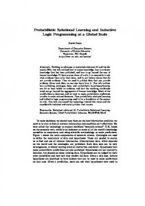
1.3 Objectives of the Thesis

E F F E C T I V E N E S S

1

Optimization

2

Encoding

3

Genetic Operators

4

Diversity

Evolutionary Algorithm Learner

6

7

Background Knowledge Sampling

Parallelization

5 Numerical Attributes

E F F I C I E N C Y

Figure 1.1: Components of an evolutionary learning system. As already stated in the previous section, the aim of this thesis is to design a ILP system that incorporates standard ILP strategies and GAs techniques. The issues of efficiency and effectiveness are central in our research. These issues are addressed along the dimensions illustrated in figure 1.1, and briefly explained in the sequel. The main features of the system for achieving effectiveness and efficiency are illustrated in figure 1.1 and explained in the following. First we will address the features regarding the effectiveness of the system and then those regarding the efficiency. Effectiveness 1. Incorporate into a GA an optimization phase based on ILP operators for optimizing individuals of the current population. This helps to guide the GA search towards regions of the search space containing good individuals (exploitation). 2. Develop a representation close to the Prolog syntax. This choice is motivated by the fact that such a representation makes the application of relational operators used in ILP and the evaluation of individuals easier. 3. Develop genetic operators that bias the search toward better hypotheses. Standard GA operators act blindly, that is they do not incorporate knowledge information about the problem. The operators we introduce act greedily. They take into consideration various possibilities, and choose the one yielding the best improvement in terms of fitness.


4

4. Develop techniques for promoting diversity in the population and good coverage of positive examples. When learning concepts with a GA based system, it is fundamental that the population be diverse and that as many examples as possible be covered. We want to assure that these two aspects are met by the population evolved by our system. 5. Introduce methods for handling numerical attributes. Many learning problems use data containing numerical attributes. Numerical attributes affect the efficiency of the learning process and the accuracy of the learned theory. Efficiency 6. Develop techniques for reducing the computational cost (in terms of time) of the learning process. More precisely, employing mechanisms for controlling the computational cost of fitness evaluation and the computational cost of the genetic search. 7. Exploit the natural parallelism of the GAs. We want to parallelize the system in order to reduce to the computational effort for carrying out the process. Points 1,2,3,4 and 6 are discussed in chapter 5. We address point 5 in chapter 6, while chapter 8 regards point 7.

1.4 Overview of the Thesis The thesis is structured in the following way. In chapter 2 we give a brief introduction to inductive logic programming. We begin by explaining the limits of a propositional representation, used for representing concepts, examples and background knowledge, and why in some cases a first–order representation is needed. We then present the basic concepts of inductive logic programming. We end the chapter by giving two examples of standard algorithms for inductive logic programming. In chapter 3, the basic notions of evolutionary computation are given. We begin by individuating four paradigms in which evolutionary computation can be divided, and by giving some history of the field. We then discuss various aspects of evolutionary computation when applied to ICL. The reasons for which the entire hypothesis space can not be considered and some method for limiting the portion of the hypothesis space to consider are then presented. The concepts of diversity, species and niches are then given. The chapter ends with an explanation on how evolutionary computation and other heuristics can be combined in order to obtain better results. Chapter 4 gives an overview of state of the art ILP algorithms based on evolutionary computation. Five systems are briefly presented. The first three

1.5. NOTATION

5

presented systems adopt the same encoding, while the other two adopt different solutions for representing candidate solutions. A description of all the genetic operators that are used by the systems is given. In chapter 5 we describe in detail the system subject of this thesis. All the basic features are presented and discussed in this chapter. We start by giving a general explanation of the system. Then we present one by one all the components, starting from the particular biases adopted for limiting the search space, and ending with the way in which a final solution is extracted. The way in which the system handles numerical values is the subject of chapter 6. We propose three alternative ways in which this can be done. In this chapter a standard way for dealing with numerical values is also briefly introduced. A number of experiments for testing the various components of the introduced system and for comparing the performance of the system with other systems are presented in chapter 7. With these experiments we have evaluated the effectiveness of some solutions adopted by the system. In chapter 8 a simple parallelization of the system is described, and some experiments are conducted for evaluating the effectiveness of the parallelization. Two case studies are presented in chapter 9. The first study does not require a first–order representation. This case regards the analysis of a medical dataset. Two problems are extracted from this dataset. The first problem is to extract rules for individuating whether a patient is satisfied by his or her relation with his or her doctor. The second problem consists in extracting rules for individuating psychiatric patients and non–psychiatric patients. If such rules can be found, this may mean that in psychiatry the doctor–patient relation is perceived in a different way. The second case study requires a first–order representation, and regards the acquisition of knowledge for individuating traffic problems on a road network. Finally, in chapter 10 we give some conclusions for this thesis.

1.5 Notation The following notation is adopted in this thesis:

denotes a set of examples;

denotes a single example; denotes a set of positive examples; denotes a set of negative examples;

denotes an individual of the population; denotes a clause; denotes the empty clause;


6

denotes a literal;

denotes a predicate; denotes a term;

denote variables. We follow Prolog notation, so in general terms starting with a capital letter denote variables, while terms starting with a lower case letter denote constants;

denotes a substitution;

! $" #

&#

denotes a query;

denotes an hypothesis;

denotes set of positive examples covered by % , where % can be either , ! or the ; denotes set of negative examples covered by % , where % can be either , ! or the ;

('*),+ .- denotes the set of individuals covering the example ; ('*)0/2143 " /$5 & /76 denotes the number " / of positive and & / of negative examples covered by an individual ; 8:9 denotes the background knowledge; ;+ % - denotes the fitness of % , where % can be either ! , or ;

Chapter 2

Inductive Logic Programming Learning from examples in FOL, also known as Inductive Logic Programming (ILP) (Muggleton and Raedt, 1994), constitutes a central topic in Machine Learning, with relevant applications to problems in complex domains like natural language and molecular computational biology (Muggleton, 1999). Learning can be viewed as a search problem in the space of all possible hypotheses (Mitchell, 1982). Given a FOL description language used to express possible hypotheses, a background knowledge, a set of positive examples, and a set of negative examples, one has to find a hypothesis which covers all positive examples and none of the negative ones (cf. (Kubat et al., 1998; Mitchell, 1997)). This problem is NP-hard even if the language to represent hypotheses is propositional logic. When FOL hypotheses are used, the complexity of searching is combined with the complexity of evaluating hypotheses (Giordana and Saitta, 2000). In this chapter we give a brief introduction to ILP. In section 2.1, we start by motivating the choice of first–order logic for describing a learning problem. Section 2.2 gives an introduction to ILP. In particular we first give some basic definitions of FOL, which are needed in the following of this thesis. We then address the problem of verifying if a given hypothesis covers an example. The way in which the space of all possible hypotheses can be ordered is then discussed. The ordering presented is exploited by many systems for ILP. In section 2.3 we give two examples of systems that can solve ILP problems. Section 2.4 concludes this chapter by summarizing the treated arguments.

2.1 Representation Language When we want to solve a problem with a computer, the first thing that should be done is to translate the problem into computational terms. In our case this means to choose a representation language and an encoding. 7

CHAPTER 2. INDUCTIVE LOGIC PROGRAMMING

8

The choice of a representation language for representing hypotheses may vary from a fragment of propositional calculus to second–order logic. While the former has a low expressive power, the latter is rather complex, and for this reason is seldom used. In this chapter we only address the representation language issue, while we will address the encoding issue in chapter 3. Car 1 2 3 4 5

Price low high low average high

Conditions average bad average good good

Age average new old new new

Power (cc)

=@?0?0? AB=@C0?0? =?D?0?FEG=D=?D? =@H0?0?FEG=@I0?D? =*HJ?D?KEL=ID?0?

Color Blue Black Red White Black

Buy Yes No No Yes Yes

Table 2.1: Features of a second hand car.

2.1.1 Propositional Representation We talk about propositional representation, when a problem can be represented by a fixed number of attributes, each of which represents a specific feature of the problem. Let us illustrate this case through an example. Suppose we want to buy a second hand car. If we are not experts in cars, we may take into consideration only a limited number of features, for example the price, the general condition, the age, the power of the engine and the color of the car. We may decide whether to buy a car or not basing our decision only on these features. Each car that we see represents an example of our problem, which is to learn the concept of when to buy a car. Each example is described by five attributes, which identify the features we consider. We could go to visit some second hand cars dealers, and collect a number of examples. We can organize the data we have collected like in table 2.1. In this case we have checked five cars. The first car had a low price, average conditions, it was of average age, had a low power and was blue, and we thought the car was a good deal. The other four cars are described in the same way. So each object is described by a limited and fixed number of attributes. We can then infer a rule for buying a car. An example of such a rule could be if conditions(good or average) and age(new or average) then buy the car.

2.1.2 First–Order Logic Representation The motivation for using first–order logic is that for some problems, e.g molecular biology (Muggleton, 1999) and natural language, propositional logic can not represent adequately the data structures. As an example, consider the molecule represented in figure 2.1. A molecule consists of several atoms, each of which is described by some properties, e.g., the molecular weight of the atom, or the charge of the atom. In addition to

2.1. REPRESENTATION LANGUAGE

9

Figure 2.1: A molecule consists of a non-fixed number of connected atoms. Each atom is described by its own set of properties.

properties relative to a single atom, there are relations among atoms. A first kind of relation is represented by links between two atoms. If two atoms are linked to each other we say that there is a bond between them. Atoms can be associated in more than one bond, and there are different types of bonds. Another example of relation among atoms are structures that can exist inside a molecule. A structure can be seen as a relation that involves all the atoms that belong to a particular structure present in the molecule. For example, from the molecule represented in the figure, it is evident that some atoms form a “ring” structure. If we want to represent such a molecule with propositional logic, we first have to fix a maximum number of attributes, which describe the properties of atoms. Not all the atoms in the molecule possess the same properties. It follows that many of these attributes will not have any value, because they describe properties that are not relative to all the atoms. Then for every relation among atoms there should be an attribute for every possible tuple of the relation. The number of attributes for a relation explodes and is polynomial in the number of available objects. Another problem is that for representing the molecule, one should also fix an order of its atoms. Without an ordering there is an exponential number of equivalent representations of a structure. These problems prohibit an efficient attribute–value representation. Instead, with first–order logic, we do not have to fix a maximum number of attributes, nor having an attribute for each possible tuple of a relation. Each atom can be described only by the properties relative to it. Relations can be represented by n–ary predicates, whose arguments are the atoms involved in the relation, and possibly the relation type. ' + For * example, '*T VU a",bound *- . between two atoms M , MON could be represented as P &RQ M MSN P &RQ


10

2.2 ILP When the language used to express examples, background knowledge and hypotheses is (a fragment of) first–order logic, ICL is called Inductive Logic Programming. ILP can be placed in the intersection between machine learning or data mining and logic programming (Muggleton and Raedt, 1994). ILP shares with the former fields the aim of finding patterns in the data and to develop tools and techniques to induce hypotheses from observations (examples). These patterns can be used to build predictive models or to get some insight of the data. ILP shares with logic programming the use of FOL for the representation of hypotheses and data. Intuitively we can then define the aim of ILP in the following manner:

W

Definition 2.1 Given are: a set of positive examples , a set of negative exX and background knowledge 8W9 of the concept amples to be learned, ex! such that ! pressed in FOL. Then the aim of ILP is to find a hypothesis ! : X covers all Y and none of the ZY . is a logic program. The basic components of FOL are called terms. Terms can be constants, variables or functions. A constant is a name that denotes some particular object in some domain. For example “4” is a constant that denotes the number four in the domain of natural numbers. A variable is a name that can denote any object of a domain. A function symbol denotes a function of arity n taking n arguments from a domain and returning one object of the For example are terms

domain. if f is an arbitrary function symbol of arity n and of the ;+ - is a term indicating a function. In addition same domain, then to terms we have predicate symbols. A predicate symbol stands for the name of a relationship between objects. Each predicate symbol has an associated arity.

Definition of.arity terms. Then + . 2.2 - aresymbol

\ n and - andLet[ + be Japredicate literals. are called the arguments of the literal.

+

M P - is a positive Literals can be positives or negatives. For+ example, + literal, which + is true if M P is true, while [ M P is a negative literal, which is true if M P - is false. We refer to a positive literal also as an atom. In this thesis, we consider hypotheses which are logic programs. A logic program is defined in the following way: Definition 2.3 A logic program is a finite set of Horn clauses. Definition 2.4 A is a clause of the form ] Horn \ clause are literals. is an atom and

^@

, where ]

In the sequel we consider clauses containing only atoms in the body (so no negation). We say that the part to the left of the arrow is the head of the clause, while the part on the right of the arrow is the body of the clause. Moreover

2.2. ILP

11

if the arguments of a clause literals are all ground terms we say that the clause is a ground clause. If a + clause consists of only the head called fact. A fact + `_ it- .isThe first fact states can be ground , e.g., M P - , or not ground, e.g., that the object M is in some relation, identified by the predicate symbol , with another object P , while the second fact states that every object + of + the domain _ `_ -b- . The is in relation with the object , and we can express this as a is read for symbol a is called universal quantifier, and the combination a : X : 8 9 every object X. In this thesis, , and are sets of ground facts. A clause has two interpretations, a declarative interpretation (universally quantified FOL implication), which defines the meaning of the clause, and a procedural one, which defines how to solve the clause.

" Example f + M - is: 2.1 The declarative interpretation of the clause

+ - dc + e -

a ` g + c + - f + M -ihj" + -b-

and its procedural interpretation is: in order to solve "

+ -

solve

c + -

and f

+ M -.

Example 2.2 The following is a logic program:

= 77 k`k`lDlDlnlnmmo,o,pp b+b+ 33 6G` q s` r 6 - 3 Gq tr 6 - k`lDlnmo,p + sr@ r - H

kl0lum\ovp +b3 Gq r 6

This is formed by two clauses. Clause 3 Glogic q r 6 - program kl0lum\ovp + r 1` isga fact. r - is its body. k`lDlnmo,p is the head of the clause 2, while ` r r are variables. is the only predicate symbol of this logic program.

During the learning process we will often need to check whether or not an induced clause covers an example. In the same way, at the end of the learning process we have to check if a whole logic program covers an example. To this aim the programming language Prolog is used. Prolog is an implementation of the logic programming paradigm. In the following we will see how this can be done, but first we have to introduce some more notions of FOL. The first notion we need is the notion of substitution. A substitution is used for instantiating a variable to a particular term of the domain.

w1yx 5 \b 5 ,z

Definition 2.5 A substitution is a finite w{ a term X{ , =~L ~ from

{ , {}1 | mapping &. variables to terms that assign to each variable Example 2.3 tions.

1jx 5 M ` 5 P z , N 1x 5 '* b 5 z

are examples of substitu-

Applying a substitution to a term , denoted as , is the result of the

simultaneous replacement of each occurrence of a variable in appearing also in with the correspondent term.


12

>1x 5 ` 5 z

1;+

>1;+

- and - . If Example 2.4 Let , then the were not simultaneous we would obtain the wrong result ;+ replacement - . Having two literals, it is sometimes possible to render them equal with an application of a substitution. If such a substitution exists, it is called unifier . In general there can be many unifiers, and among them a most general one can be identified.

Definition 2.6 Let two substitutions. Then F , N ,N ifbethere . we say that .K1is more general than N , exists a substitution such that N.

}

Definition 2.7 Let a substitution. We say that is } and N and N be1 two N . literals, } and N are unifiable a unifier for iff We also say that via . is the most general unifier (mgu) if is more general of all the other and N . unifiers of

}

+

+

Example 2.5 Let and N be " P - and " M P - respectively. } } and N Then is a unifier for and N . Moreover is the mgu for . We can question a logic program through the use of queries:

Definition 2.8 A query to a logic program is a clause of the form { where , =(~G~ & , are literals.

+

W1Bx 5 M z

^b

+ `

- can be interpreted as the inquiry -? A query When we pose a query to a logic program, a resolution procedure, called SLD (Selection rule driven Linear resolution for Definite clauses) is applied in order to verify if the query is satisfied by the logic program. The SLD resolution uses the procedural interpretation of the clauses forming the logic program for looking if the query has a successful derivation. If such a derivation exists then the answer will be “yes” otherwise the query fails and the answer will be “no”. A SLD is a sequence of derivation steps. If we pose a query SLD ` to a logic .derivation program , then a derivation step will consist of the following operations: { , =Z~~ & , in the query; such that its head can be unified with { ; select a clause in select the mgu for the query and the head of ; { replace in the query with the body of the clause, and apply mgu to the

1. select an atom 2. 3. 4.

resulting query;

In steps 1 and 2, the order in which atoms in the query have to be solved (selection rule) and the order in which clauses of the logic program are used in the derivation need to be specified in order to render the resolution deter

ministic. If the derivation ends with the empty clause, denoted by , then it

2.2. ILP

13

is a successful derivation. If the derivation ends with a query in which the selected atom is not unifiable with any clause in the logic program, then it is a derivation of failure. A derivation can be also infinite. is a logic program from which a query can be derived In general, if B . in zero or more resolution steps, then we denote this by An important property of resolution is that only logical consequences can be derived. This results is known as soundness of resolution. In general, a formula logically implies another formula any model for is also q 1 . Awhenever a model for , which we denote by model for a formula is an interpretation of the logical language under consideration that makes the formula true. For Horn clauses, we can restrict our attention to so–called least Her determines brand models. Every Herbrand model for a logic program a set of ground facts that are true in . The least Herbrand model of a logic , denoted as n is the unique set that contains exactly all ground program . Thus logically implies atoms that are true in all Herbrand models for 1 q a ground atom ] ( ] iff n contains ] . Once we have defined a selection rule, the totality of SLD derivations for a given query and logic program can be represented by a SLD tree. Each branch of a SLD tree is a SLD derivation via the selection rule. The nodes of the tree are queries with a selected literal. Each node in the tree has exactly one son for each clause that unifies with the selected literal of the query contained in the node. In Prolog the procedural aspect is implemented using a depth–first search strategy through the clauses defined by a logic program, and by choosing always the first unresolved literal in the query. Prolog builds all possible derivations for the query until it finds a successful one, or until all possible derivations have been tried. In the latter case the query fails.

is the following simple logic program: \kJum\ + u - luk.mou + u - kJ ¡m + - = H ¢luk.`m\o$ + V£.¤@¥¦ - ¢luk.`m\o$ +¨§ kD©`ª«@m¬*m - uI ¢luk.`m\o$ + m¬*mD*¥\¦ - ®Xk. ¯m + °£J - ±C ®Xk. ¯m + ¥\¦ - ²O®Xk. ¯m +³§ k0©ª - ´ \mXk. ¡m + m¬.m -

Example 2.6 Suppose that

\k.µnm + @¥¦ -

and we pose the query cessful derivation found by Prolog is:

to

. Then the first and only suc-

\k.µnm + *¥\¦ - ¶ E ·`hº ¸ ¹ " M c @& + PV»» - MO» + - ¶bE ¼gh ¸ ¹ N MO» + '* - ¶¾E ½\h ¸ ¹

where the selected literal in each derivation the se 1Áx 5 isPV»Âunderlined, _ { step of´ ,the lected clause is shown like , =~¿À~ and » z , N 1Áx 5 '* z ,


14

.K1Ãx z . N . K1Äx 5 '* 5 PV»» z is the computed answer substitution. In this ; bÅ c + P V»» - N *1; M bÅ c + '* PV»Â» - is the computed instance of the case M

query. Note that if we exchange the second and the fourth clause then the first derivation found by Prolog for the query will be of failure. \kJum\ + V£.¤*¥\¦ In the same way, we can verify that also the ground query x + G Æ \ . k µ n m ° J £ ¤ @ ¥ ¦ z

has a successful ( ) , while the query - fails. Finally, \k.µnm + m¬*mD@¥¦ derivation if we want to know who is the father of who \k.µnm + u - . The computed answer substitutions we x*pose the query will 5 °£J¤u 5 ¥\¦ z and x*5g§ k0©ªv$ 5 m\¬.m z . be We now have all the instruments for verifying the conditions given in definition 2.1. We can invoke Prolog every time we need to check if a logic program covers an example by posing queries. If Prolog finds a successful derivation for the query than the example is covered, otherwise Here we exploit the itisisanot. completeness of the resolution, that says that if logic program and ] a q 1 ] ;«; ÇÆ x ] z . ground fact, then

Example If is the first clause of the logic program shown in example 2.6, 8W9 is2.7formed and by the other same logic program, then we have \k.µnm + °£J¤facts @¥¦ of- isthecovered seen that the example found - posedProlog \k.µnm + °£Jby¤@¥,¦ because a successful derivation for the query to the logic and 8:9 . In the same way, we know that program formed by the union of 1 + \ J k u \ m V . £ ¤ * \ m . ¬ m -. does not cover N The two main advantages of ILP are: 1. the use of a FOL representation; 2. easy incorporation of a background knowledge of the domain; The first point is important because, as we have seen, many domains can only be expressed in first–order logic and not in propositional logic. The second point is important because the use of domain knowledge is essential for achieving intelligent behavior. FOL offers an elegant formalism to represent knowledge and hence to incorporate it in the induction task. The background knowledge is a knowledge common to several examples.

2.2.1 Ordering the Hypothesis Space The ILP problem can be seen as the problem of searching a hypothesis space for a hypothesis that matches the conditions mentioned in definition 2.1. However, a drawback of a first–order logic representation is that the hypothesis space associated to this representation is usually much larger than the search space associated with a propositional representation. This is because the number of first–order logic candidate solutions is much higher than the number of propositional logic candidate solutions. For this reason the hypothesis space is typically limited by a set of inductive biases, as we will see in sections 2.3.1

2.2. ILP

15

and 2.3.2 and in chapter 3. Another aspect that is used is an implicit ordering of the hypothesis space. In fact, the search space can be structured with a general-to-specific ordering of hypotheses.

!w

!

!

more general than a hypothesis N , and N Definition 2.9 A hypothesis !s , if all theisexamples ! is more specific than covered by N are also covered by !s .

!s be \k.µnm + $ - lnkJmou + u - MO» + - . and ! N be \Example kJum\ + 2.8 °£J Let - ul k.mou + V£. - kJ ¡m + - v!s is more general than ! N , be! !w will cover all the cause it will cover more examples than N . In particular ! ! examples covered by '* N . In fact N covers only examples for which the second

. argument is equal to !w

+ - , ! N be " + M - and ! be " + M P - , then we have N and ! and that ! N is more general that ! .

Example 2.9 Let be " s ! ! that is more general than

We can imagine the hypothesis space structured in this way. For example, if and we have only the predicate symbol " of arity two, the two variables and the two constant M and P , as in the example 2.9 our hypothesis space, consisting of just one atom, can be viewed in figure 2.2 as a lattice with the general to specific ordering.

ÉÊ É " + M ` Ë Ë ÍÎ Í +" M È ÉÊ M -É

É É " Í ËÍ ËÉ É

É ÉÍ ÉÍ ÉÍ + ÍÎ M Í Ï Ï ÏÉ É É Ï ËÉ Ë«É Ì " +M P -

" + ÉÍ ÍÉ ÓË ÓË ÓË Ó Ó Ë Ë Ë«Ì Ó Ó È+ ` " " + P ` É Ï Ñ Ë É Ï Ï Ï Ï É ÏÉ ÑÒ ÑÏÉ ÉÏ ÉÏ ÉÊ É É É Ï«" Ð + P M -

G

Ó Ó «Ó Ô " + P ÉË ÉË ÉË É Ï Ï Ï«Ð Ë«Ì È " +P P -

È

S

Figure 2.2: Hypothesis space for a simple language. The general to specific order is indicated by the arrow on the right of the tree structure. In the figure another means “more general”. instance + ` - For ` -thjfrom - is more "an+ arrow " + M a literal - meanstothat " + `literal general than " M . Many systems for ILP exploit this ordering of hypotheses in the operators they use for moving in the search space and for deciding the direction in which the search is performed. The operators vary from system to system, depending on the approach used, the problem to solve, the ideas of the authors and so on. An operator basically receives a hypothesis, changes it in some ways and returns the changed hypothesis. Some systems start the search from a specific hypothesis, which is then generalized during the learning process. This approach is called bottom-up. Alternatively a top-down approach can be used.

16


In this case the learning process starts with a general hypothesis which is then specialized to fit the training examples. An operator used in many ILP systems, is the inverse resolution. To give a flavor of how this operator works, we will describe it for the propositional form, while for details about the inverse resolution in FOL the reader can refer to (Muggleton, 1995). in this method is inverting the resolution What isN , done rule. Given rules and the resolution operator constructs a clause . £ ¦ o . £ 7 Ö × g Ø ° J k . Ù ¦ o u . £ X m which is derived from and N . For example, if is Õ Õ×ØgÖup.Ù Õ Ø V . k . Ù ¦ o n J £ } m × g Ø u Ö J p Ù J £ ¦ o J £ 7 Ö R and N is [ then will be Õ Õ Õ and . . The inverse resolution operator then produces N starting from The inverse resolution operator is not deterministic. This means that in general there are multiple choices for N . A way for limiting the number of choices is to restrict the representation language to Horn clauses and to use inverse entailment. The idea inverse entailment is to change1 the entail8:9ÛÚ!Üq 1 behind 8W9jÚ [ q [ ! . The into the ment constraint equivalent form previous constraint says that from the background knowledge and the negation of the classification of an example, the negation of a hypothesis explaining the example can be derived. Thus, from the modified constraint one can use ! a process similar to deduction to derive a hypothesis . This operator will be used by the system described in section 2.3.2. Other examples of operators used for moving in the hypothesis space are represented by the operators used by evolutionary systems. We will see examples of evolutionary operators in chapter 3.

2.3 Two Popular ILP Systems To conclude this chapter, in the next two sections we briefly describe two well known systems for solving ILP problems: FOIL (Quinlan, 1990) and Progol (Muggleton, 1995; Muggleton, 1996). We have chosen to present FOIL because it represents probably the most popular system for ILP, and Progol because of its application to a number of real life ILP problems.

2.3.1 FOIL FOIL searches the hypothesis space using a top-down search approach and adopts an AQ-like sequential covering algorithm (Michalski et al., 1986). The system first induces a consistent clause and stores it. All the positive examples covered by the learned clause are removed from the training set, and the process is repeated until all positive examples are covered. When a clause needs to be induced, the system employs a hill climbing strategy (for an explanation of hill climbing the reader can refer to e.g., (Russel and Norvig, 1995)). FOIL starts with the most general clause, consisting of a clause with an empty body and head equals to the target predicate. All the arguments of the head are distinct variables. In this way this initial clause classifies all examples as positive. The

2.3. TWO POPULAR ILP SYSTEMS

17

clause is then specialized by adding literals to its body. Several literals are considered for this purpose. The literal yielding the best improvement is added to the body. If the clause covers some negative examples then another literal is added. This process is called hill climbing because it proceeds with small steps toward a local best hypothesis. In figure 2.3 a scheme of the algorithm adopted

+

A LGORITHM Ý(Þ 1 Initialize the clause 2 while the clause covers negative examples 3 do Find a “good” literal to be added to the clause body; 4 Remove all examples covered by the clause; 5 Add the clause to the emerging concept definition; 6 If there are any uncovered positive examples then go to 1; Figure 2.3: The scheme of the algorithm adopted by FOIL. by FOIL is presented. In steps 2 and 3 the hill climbing phase is performed. The representation language of FOIL is a restricted form of FOL, that omits disjunctive descriptions, and function symbols. Negated literals are allowed in the body of clauses, where the negation is interpreted in a limited way (negation by failure). The evaluation function used by FOIL to estimate the utility of adding a new literal is based on the number of positive and negative examples covered before and after adding the new literal. More let be the clause to has to be added and ß theprecisely, which a new literal clause created . The information gain function used is then the following: by adding to

à\o\£ Õ Jk ¦o 1>á _â + » '@ã ä åSæ Eç» '@ã å ä å å äåSæ åSæ ä where "$è "$è æ &R Zè ß &Rè æ is the number and negative examples á _ of the positive covered by and , respectively, is the number of positive examples cov ered by that are still covered after adding to . The add operator considers literals of the following form:

é + w* N sê -

+ wJb N \bsê - , where { ’s are variables of

and [ the clause or new variables;

ë é { 1 W é { 1 _

X{1 | W ë , for variables of the clause; { 1 | _ , where { is a variable in the clause and _ and or

appropriate constant;

é { ~ ë , { A ë , { ~ )

{

)

{

ë

is an

and A , where and are clause variables that can assume numeric values and v is a threshold value chosen by FOIL.


18

There is a constraint on literals that can be introduced in a clause: at least one variable appearing in the literal to be added must be already present in the clause. Another restriction adopted by FOIL, is motivated by the Occam’s razor principle (Blumer et al., 1987). When a clause becomes longer (according to some metric) than the total number of the positive examples that the clause explains, that clause is not considered as a potential part of the hypothesis any more. There is also another bias on the hypothesis space, and it is the upper bound represented by the most general clause initially generated. In fact all the clauses that are generated are more specific than the initial one.

2.3.2 Progol Progol uses inverse entailment to generate one most specific clause that, together with the background knowledge, entails the observed data. This clause is to bound a top-down search through the hypothesis space with the constraint that only clauses more general than the initial bound are considered.

+ c '@ãO'

A LGORITHM »8:- 9 ® 1 ì 1 If return ; 2 Let e be a selected example in ; 3 Construct a most specific clause í for using inverse entailment; 4 Construct clause from í ; 8:a 9 “good” 5 Add to ; 6 Remove from all the examples that are now covered; 7 Go to 1; Figure 2.4: Covering algorithm adopted by Progol. The emerging hypotheses are added to the background knowledge and the algorithm is repeated until all the positive examples are covered. Progol uses a sequential covering algorithm, illustrated in figure 2.4, to carry out its learning task. For each positive example that is not yet covered, it first searches for a most specific clause, here denoted by í , which covers (line 3). For doing this it applies i times the inverse entailment, where i is a parameter specified by the user. In line 4 a ]Zî strategy is adopted for finding a good clause starting from the most general clause. According to this strategy, a number of clauses are constructed starting from the initial clause. The clause that is considered to be the best is then chosen and the process is repeated. Progol uses -subsumption for ordering the hypothesis space. A clause E subsumes N iff there exists a substitution of aisclause N ( esuch ï2 Nthat the is set literals of contained in the set of literals of ), ( more ç N ). The refinement operator maintains general than N , written also

the relationship clause . Thus the search í for every considered í , there exists is limited to the bounded sub-lattice í . Since Ä ï a substitution such that í . So for each in , there exists a literal

2.4. CONCLUSIONS

ß

ð1 ß

19

in í such that refinement operator has to keep track of . ß The and a list of those literals in í that have a corresponding literal in . Any clause that subsumes í corresponds to a subset of literals in í with substitutions applied. Among all the refinements the one that is considered the best is chosen, according to an evaluation function, and the process is repeated. is:The evaluation function used to measure the goodness of a candidate clause

;+ - 1 " è E + & èñ » ã Å èòñ Å è ãÅ where » è is the length of , defined as the number of literals in minus 1, Å and è is the expected number of further atoms that have to be added to the Å body of the clause. è is calculated by inspecting the output variables in the

clause and determining whether they have been defined. The output variables are given by a user supplied model.

A first bias on the hypothesis space is represented by the upper bound and by the lower bound í . A second constraint is the use of the head and body mode declarations together with other settings to build the most specific clause. With a mode declaration, the user specifies for each atom used the modality in which an argument can be used. So for example it can be specified that a particular argument is an input variable, or an output variable, or again a particular constant. Progol imposes a restriction upon the placement of input variables. Every input variable in any atom has to be either an input variable in the head of the clause or an output variable in some atom that appeared before in the clause. This imposes a quasi-order on the body atoms and ensures that the clause is logically consistent in its use of input and output variables.

2.4 Conclusions This chapter provided an brief introduction to ILP. We have first seen how for some classes of problems a propositional representation is not adequate. This motivates the use of first–order logic for representing data. In chapter 9 another example of problem for which a first–order representation is needed is given. ILP can be seen as a search problem through a hypothesis space, where structures are represented in first–order logic. The objective of the search is to find a hypothesis that covers all the positive examples and none of the negative ones. We have seen how Prolog can be used for checking whether a given hypothesis covers an example or not. A first–order representation has a great expression power, but this implies that the hypothesis space to search is huge. A strategy for overcoming this is to consider the general-to-specific ordering of the hypothesis space. In this way the hypothesis space can be structured using the concept of generality given in definition 2.9. This ordering allows to search through the hypothesis space in a more efficient way, by means of specialization and generalization operators. The description of two standard ILP algorithms that take advantage of the general-to-specific ordering of the hypothesis space concluded this chapter.


20 Algorithm

Quality function

FOIL

Information Gain

Progol

"$è , &Rè , » ã Å è , Å è

Language FOL without function symbols and disjunctive description

í

Operators Add literals with at least one variable already in clause Inverse entailment Refinement operator

" è and & è are the Table 2.2: Summary of features of FOIL and Progol. In table ãÅ number of positive and negative examples covered by , respectively. » è Å è is the length of and is an estimate of how many literals still need to be added to . In table 2.2, we summarize the main features of the two algorithms. In particular we summarize the features that are considered when assessing the quality of a candidate clause, the language adopted by the two systems and the operators used. For assessing the quality of a candidate clause, FOIL uses the information gain obtained when a new literal is added to the body of the clause. The literal yielding the best gain is added to the body of the clause. Progol uses a similar strategy. Once the refinement operator has generated a number of candidate solutions the one with higher quality function is chosen and further refined. The quality function used by Progol uses information regarding the coverage of the candidate solution, its length and an estimate of how many refinement steps have to be performed in order to obtain a final clause. The language adopted by FOIL is a restricted form of first–order logic, where function symbols and disjunctive descriptions are not allowed. The language adopted by Progol vary from clause to clause, and is determined by the most specific clause built with the inverse entailment operator. Both systems adopt a greedy search strategy for finding good candidate solutions. This gives the systems a good exploitation power, i.e., they are very good at fine-tuning candidate solution, but have rather poor exploration power. This may prevent the systems to escape from local optima.

Chapter 3

Evolutionary Computation Evolutionary Computation (EC) is a population–based stochastic iterative optimization technique based on the Darwinian concepts of evolution described in the “The origin of species” (Darwin, 1859). Inspired by these principles, like survival of the fittest and selective pressure, EC tackles difficult problems by evolving approximate solutions of an optimization problem inside a computer. An algorithm based on EC is called an evolutionary algorithm (EA). EC has been applied to find solutions of problems in a variety of domains, e.g., planning (Goldberg and Robert, 1985; Fogel, 1988; Jakob et al., 1992), design (Bentley and Corne, 2001; Bentley, 1999; Divina et al., 2003a), scheduling (Davis, 1985; Yamada and Nakano, 1992; Corne et al., 1994), simulation and identification (Roosen and Meyer, 1992; Gehlhaar et al., 1995; Tanaka et al., 1993), control (KrishnaKumar and Goldberg, 1990; Spencer, 1993) and classification (Holland, 1987; Fogel, 1993; Keijzer, 2002). In this chapter we give some basic notions and principles of EC. The chapter is structured as follows. In section 3.1 we illustrate EC by means of a simple example. In section 3.2 the four paradigms in which EC is usually divided are explained. In section 3.3 we discuss the various components of EC applied to the ICL problem. We start by discussing the representation language and encoding that can be used. We then address the problem of how to evaluate the goodness of an individual, and which aspects of an individual are usually taken into account when assessing the goodness of an individual. Variations operators are then discussed, and some examples are given. In section 3.4 we see how and why the portion of the hypotheses space searched can be limited by means of inductive biases. Section 3.5 addresses the notions of species and niches formation, and the problem of maintaining diversity in the population evolved by an EC system. In section 3.6 we briefly motivate and present the concept of hybrid EC. Section 3.7 presents a summary of the discussed aspects. For a more detailed introduction to EC the reader can refer to (Bäck et al., 2000a; Yao, 2002; Eiben and Smith, 2003a). 21

CHAPTER 3. EVOLUTIONARY COMPUTATION

22

3.1 Introduction to Evolutionary Computation Given an optimization problem, all EAs typically start from a set, called population, of random (candidate) solutions. These solutions are evolved by the repeated selection and variations of more fit solutions, following the principle of the survival of the fittest. We refer to the elements of the population as individuals or as chromosomes. So each individual encodes a candidate solution. Solutions can be encoded in many different ways. A typical example is represented by binary string encoding, where each bit of the string has a particular meaning.

õGö ó 1ô G õGö ó 3ô G

õGö ó 2ô G õGö ó 4ô G

õGö ó 1ô ÷ G õGö Ñ ó 3ô G

Ñ

÷

÷Ñ

Ñ ÷

Ñ

õGö Ñ óG2ô

÷

÷ õGö óG4ô

Figure 3.1: Two candidate solutions for the problem of example 3.1.

Example 3.1 Suppose we have a graph made of four nodes, and that each node can be connected to each other. We consider the problem of connecting the nodes in an optimal way, according to some criterion. Two candidate solutions are given in figure 3.1. We could encode these solutions in binary strings in the following way: we fix an order for the possible connections, and associate a bit in the binary string to each possible connection. If a bit relative to a connection is set to 1 then the connection is present in the graph. In total we need 6 bits for representing candidate solutions. We may then consider the following order for connections: (1-2),(1-3),(1-4),(2-3),(2-4),(3-4). The solution depicted on the left hand side of figure 3.1 is then encoded by the string 110011, while 001111 is the binary string relative to the solution proposed on the right hand side of figure 3.1. The binary strings of example 3.1 represent the genotype of the individuals with phenotype represented by the two graphs of figure 3.1. In general, with the term phenotype we refer to an object forming a possible solution within the original context, while its encoding is called genotype. To each genotype must correspond at most one phenotype, so that the chosen encoding can be inverted, so that genotypes can be decoded. Individuals are typically selected according to the quality of the solution they represent. To measure the quality of a solution, a fitness function is assigned to each individual of the population. Hence, the better the fitness of an individual, the more possibilities the individual has of being selected for

3.1. INTRODUCTION TO EVOLUTIONARY COMPUTATION

23

reproduction and the more parts of its genetic material will be passed on to the next generations of individuals. Example 3.2 The fitness for individuals of example 3.1 could be a measure of how well the connection criterion is met by individuals. The selected individuals are modified by means of some variation operators, described in section 3.3.4. From the reproduction phase, new offspring are generated. Offspring compete with the old individuals for a place in the next generation. Typically offspring replace some of the worst individuals in the population, based on the fitness. Another replacement strategy is to use the concept of age, so older individuals are replaced by new individuals.

ø th generation ú ùú ù ú ú ùù ù ú ú ú ùú úú ú ú ú ú ú

û

Variations

ü ønýÿþ th generation ú ù ù ù û ú ùù ù ú ú ú ú ú ú ú

Figure 3.2: In the th generation selected individuals are represented by black circles. Offspring are inserted in the next generation replacing bad individuals. Offspring are represented by . A graphical representation of an evolutionary step is given in figure 3.2. The oval on the left hand side represents the old population at the th generation, while the right hand side oval represents the new population. Individuals in the th generation are represented by circles, where black circles represent individuals that have been selected for reproduction. These individuals mate by means of some + genetic variations and produce offspring, represented in the figure by . In the ñ = - th generation the created offspring have replaced some of the old individuals. The process is iterated until a stopping criterion is met. Examples of stopping criteria are setting a maximum number of generations or iterating the process until a good enough individual is generated. For generating new individuals typically two kind of operators are used: crossover and mutation. In simple terms crossover swaps some genetic material between two or more individuals, while mutation changes a small part of the genetic material of an individual to a new random value. Example 3.3 Suppose two individuals from the problem presented in example 3.1 are selected, and let these individuals be those represented in figure 3.1

1 0= =? q ?u=0= N 1 ?0?n= q D= =0=

Then an application of crossover may generate the two new individuals:

24

õGö ó 1ô G õGö Ñ ó 3ô G

Ñ

Ñ

Ñ

Ñ

õGö Ñ óG2ô


õGö ó 1ô ÷ G

õGö ó 4ô G

õGö ó 3ô G

÷ ÷

õGö ó 2ô G

÷ ÷

÷ õGö óG4ô

Figure 3.3: The two offspring obtained by an application of one-point crossover to the individuals of example 3.1.

ß

ß 1 D= =? q =0=D= ßN 1 ?D?n= q n? =D=

encodes the situation depicted on the left hand side of figure 3.3, and encodes the situation shown on the right hand side of figure 3.3.

ßN

In the above example a so called one-point crossover has been used for creating two new individuals, from two selected individuals, called parents. q The operator selects a point inside the two strings, denoted by in the example, and produces the offspring by exchanging the substrings of the parents. We will see other examples of crossover in section 3.3.4. The combined application of selection and variation generally leads to improving fitness values throughout generations (Eiben and Smith, 2003b). Evolution is often seen as the process of adaptation to an environment. So fitness can be seen as how the environmental requirements are matched. The better the fitness of an individual the better the individual matches these requirements, and this increases viability, which means that the individual will have more chances to reproduce. So at each generation the population will become more and more adapted to the environment. If we are solving a problem with EC, this means that the population will get closer and closer to the solution.

3.2 Four Paradigms of EC Four main paradigms of EC can be identified (Eiben and Smith, 2003a): Evolution Strategies (ES) was introduced in (Rechenberg, 1973). ES typically use an individual representation consisting of a vector of real numbers. ES originally relied most on mutation as main exploratory search operator, but nowadays ES use also crossover. Evolutionary Programming (EP) was first introduced in (Fogel et al., 1966). EP was originally introduced for developing finite state automata for solving specific problems. Nowadays EP is often used to evolve individuals consisting of real-valued vectors. EP does not use crossover.

3.2. FOUR PARADIGMS OF EC

25

Genetic Algorithms (GAs) were introduced by John Holland in (Holland, 1975). GAs typically rely on crossover for exploring the search space. Mutation is considered as a minor operator, and is applied with very low probability. The classic representation used in GAs is a binary string one, however nowadays other kind of representations, such as real-valued strings, are also adopted. Genetic Programming (GP) was introduced in (Koza, 1992). GP is often described as a variant of GAs. In GP individuals represent some sort of computer programs, consisting not only of data structures, but also of functions applied to those data structures. Individuals typically are tree structures. Within each paradigm several different algorithms exist, with different features. For this reason the distinction between paradigms is not always so straightforward. More and more methods developed for a particular paradigm are also adopted by other ones.

+

A LGORITHM Z]ðEç 1 initialize population; 2 evaluate each individual in population; 3 repeat 4 select parents; 5 recombine pairs of parents 6 mutate the resulting offspring; 7 evaluate offspring; 8 insert offspring in the population; 9 until (stopping criteria) 10 Extract solution from population; Figure 3.4: A general scheme of a GA or a GP. A general scheme of a GA or GP is shown in figure 3.4. In the scheme, the first operation done is the initialization of the population. This can be done at random or with some different strategies. Then each individual of the population needs to be evaluated. Individuals are then evolved (the repeat statement). In step 4 a number of individuals are selected from the population. Selected individuals are allowed to generate offspring. Offspring are generated with the application of crossover and mutation in steps 5 and 6. Both crossover and mutation are applied with a given probability, called crossover and mutation rate respectively. They are then evaluated and inserted in the population. The process is iterated over a number of generations, until a stopping criterion is met.


26

3.3 Various Components of EC In the following we address various aspects of EC when used for ICL. In particular we discuss the representation of individuals, how to assess the quality of individuals and the operators that can be used for selecting individuals and moving in the search space.

3.3.1 Representation Language and Encoding In chapter 2, we have seen how important the choice of a representation language is. Once we have a representation language, we need to decide how to encode candidate solutions. An individual can encode a single rule or a set of rules, e.g., a logic program. Whatever the representation used, rules need then to be encoded into individuals. At this aim, various solutions can be adopted, e.g binary strings, real-valued strings, tree structures, high level encoding, etc. In chapters 4 and 5 we will see different solutions adopted for encoding rules.

3.3.2 Evaluation of Individuals In simple terms what characterizes a hypothesis (candidate solution) as good is how well it performs on the training examples and a prediction of how well its behavior will be on unseen examples. For instance, a hypothesis covering several positive examples and no negative examples could be considered as a good hypothesis. A fitness function is used to measure the goodness of a hypothesis. Several properties can be used for defining a fitness function, like: completeness, consistency and simplicity.

!

!

Definition 3.1 Let be an hypothesis. the positive examples.

!

!

is said to be complete iff

Definition 3.2 Let be an hypothesis. cover any negative examples.

!

is said to be consistent iff

covers all

!

does not

Completeness and consistency are two properties that almost all evolutionary inductive learning systems incorporate in the fitness function. E inconsistent region

D

A

C concept to learn

incomplete hypothesis

B

Figure 3.5: Illustration of incompleteness and inconsistency.

3.3. VARIOUS COMPONENTS OF EC

27

Example 3.4 An illustration of both an incomplete and an inconsistent hypothesis is given in figure 3.5. The to be found is represented by the area 8 .concept The oval in the figure represents an incomplete identified by the points ] but consistent hypothesis, since it fails to cover all the region identified by the target concept, but it does not cover any portion of the that does not be8 region long to the target concept. Instead, the rectangle ] represents a complete but inconsistent hypothesis, since it covers all the region relative to the target concept, but it also covers some portion of the region that does not belong to the target concept. Simplicity is a concept often used following the Occam’s razor principle, which advocates to prefer the simplest hypothesis that fits the data. One rationale explanation for this is that there are fewer short hypotheses than long ones, and so it is less likely that one will find a short hypothesis that coincidentally fits the data. There are many ways for defining simplicity, e.g.,: Short rules. Prefer shorter rules over longer ones. The length of a rule depends on the representation used, and so the same rule could be considered short by a learner and long by another one. MDL. This is a more general concept, since it uses a notion of length that does not depend on the particular representation used. According to the Minimal Description Length (MDL) principle (Rissanen, 1989) the best model for describing some data, is the one that minimizes the sum of the length of the model and the length of the data given to the model. Here by length we mean the number of bits needed for encoding a model or the data. Information gain. Information gain (Quinlan, 1986) is a measure of how a change in a hypothesis affects its classification of the examples. This principle when incorporated in the search strategy of a method like in decision trees, biases the search toward shorter rules.

3.3.3 Selection At each generation, a number of individuals are selected in order to reproduce and generate in this way a new generation. Individuals can be selected in many different ways. Selection is a stochastic process: fitter individuals have higher chances of being selected, but also weak individuals have a chance to become a parent. Examples of selection mechanisms are ranking selection, tournament selection and roulette wheel selection. For more details on selection mechanisms the reader can refer to (Bäck et al., 2000a; Bäck et al., 2000b; Goldberg and Deb, 1991; Blickle and Thiele, 1995). Ranking selection was proposed in (Baker, 1985). Every individual of the population is given a rank between 0 (less fit) and 1 (most fit). The higher the rank of an individual the higher the probability the individual is selected. In tournament selection n individuals are randomly selected from the population

28


and the fittest is selected. The parameter n determines the tournament size. A common value for n is 2.

+

) T á

R OULETTE W HEEL S ELECTION Þ á &RQ Q MO» á ) T R & Q Q 1 á ' = number of Þ MO» á _ c = array ofr dimension 2 {

{ ; &R á*áD+ { ' ; &R á@áF{1 3 r¾r / á _ ' c 1 { r¾·r 4 + Ú + ~ á .- { r¾r /"! 5 for A>= á _ ' c { 1®á _ ' c { ñ { r¾r 6 do 1 ñ = 7 c M &RQ '*Û1 random number between 0 and 1 8 á _ ' c { < c M &RQ '* ~ á _ { 9 return such that

'c{

Figure 3.6: á Algorithm roulette wheel selection mechanism. á _ ' c array istheassociated _ ' c { of theimplementing { to the relative individual . Each entry

Also in the roulette wheel mechanism n individuals are randomly selected from the population. A roulette wheel is built, where the sector associated to each of the n selected individuals is proportional to the fitness of the individual. Individuals with higher fitnesses have more probability of being selected, having wider sectors associated to them. The roulette wheel selection mechanism can be implemented by the algorithm shown in figure 3.6. First á _ the 'c, sum of all the fitnesses of the individuals is computed. Then a vector, is constructed, which represents the sectors of the roulette wheel. A random number is generated, the individual whose sector is the one individuated by the random number is selected. In chapter 4 and in chapter 5 we will see some examples of application of the roulette wheel selection.

Example 3.5 Suppose that three individuals , N and are randomly selected from the population. Let the fitnesses the three individuals be the á _ ' c is of ones shown in figure 3.7. The array then equal to 0.6 0.9 1.0 where and 1.0 are the{ upper bounds that delimit each sector. Each ená _ 0.6, ' c { 0.9 try is associated to , =e~ ~ I . A random number between 0 and 1 is generated and an individual is selected. It can be seen that has more chances of being selected, since its sector is wider. The array can be seen as the roulette wheel shown in figure 3.7, the dimension of the sectors is á _ where

' c { . The equal to the dimension of the sectors random seed can be seen as the ball used in a roulette wheel. The roulette wheel is spun and the individual associated to the sector where the ball has stopped is selected.

3.3. VARIOUS COMPONENTS OF EC

; &R *á áS+ ; &R *á áS+ ; &R *á áS+

- 1 ? N- 1 ? - 1 ?

29

±

Ñ Ñ # # N

I

=

Figure 3.7: An example of roulette wheel for three individuals,

, N

and

.

3.3.4 Variation Operators From selected individuals, offspring are generated, by means of the application of some variation operators to the parents. The most common variation operators are crossover, or recombination, and mutation. Crossover operators take two or more individuals as an input, and return two or more offspring. Offspring are obtained by swapping some parts of the parents. The choice of what parts of each parent are combined, and how these parts are combined depend on random drawings. The principle behind crossover is that by mating two individuals with different but desirable features, an offspring that combines both of these features can be created. Mutation operators receive a single individual. A small part of the individual is changed, and the new mutated individual is returned. Mutation has the role of guaranteeing that the search space is connected. In the following we will see an example of classical mutation operator. In chapter 5 other mutation operators are introduced. Variation operators can be divided into two classes: standard GA operators and GP operators. The first class of operators, GA operators, act on bit strings. We have already seen an example of crossover, called one-point, in example 3.3. Other examples of crossover operators are the two-point crossover, where two points inside the parents are used, and the uniform crossover, which combines bits sampled uniformly from the two parents. Example 3.6 An example of two-point crossover is the following: given the two parents

1 0= =D= q =0=D=0=0=D=0=D= N 1 ?0?D? q 0? ?D?0?0?D?0?D?

q =0=0= q ?0?0?

two points are randomly selected inside the strings. The points are denoted by q . With the application of the two-point crossover we obtain the two offspring:

ß 1 0= =D= q ?0?D?0?0?D?0?D? ßN 1 ?0?D? q 0= =D=0=0=D=0=D=

q =0=0= q ?0?0?

Example 3.7 An example of uniform crossover is the following: given the two parents

1 = q= N 1 ? q?

q= q?

q= q?

q= q?

q= q?

q= q?

q= q?

q= q?

q= q?

q= q?

q= q?

q= q?

q= q?


30

an application of a uniform crossover may produce the following two offspring:

ß 1 ? q = ßN 1 = q ?

q= q?

q= q?

q? q= q? q= q? q=

q= q?

q= q?

q? q? q? q= q= q=

q? q= q= q?

Example 3.8 An example of a classical mutation operator is the following: given the individual

1 =0=0=D= ?0?D?0?0?D?n=D=0=0=

a mutation operator can change the fourth bit and the resulting individual is:

ß,1 =0=D=? ?D?0?0?D?0?u=0=0=D=

The second class of operators, GP operators, act on tree structures. A crossover operator will then create offspring by exchanging subtrees of the parents. Example 3.9 If the two selected individuals are those shown on the left of the arrow in figure 3.8 then a crossover may produce the two offspring shown on the right of the arrow.

$

&

$ & %

Ñ(% '

) ' )+*

÷

' &

*

'

$ & %

% $

û $

'

&

$ & %

Ñ(% '

' & '

) ' ),*

$ & %

÷

*

% $

'

Figure 3.8: Example of GP crossover. The dark part of the two parents are swapped.

Example 3.10 If a selected individual is the one shown on the left of the arrow in figure 3.9, then an application of a GP style mutation may produce the individual shown on the right of the arrow.

3.4 Biases on the Search Space If we want to assure that a solution is found, it is obvious that the unknown target concept must be contained in the portion of the hypothesis space that is searched. Using a hypothesis space capable of representing every learnable concept could seem the solution, but this would lead to a very large search space. To illustrate this, consider a learner that uses examples described by a set of attributes. In general, in this setting, an unbiased hypothesis space

3.5. DIVERSITY, SPECIES AND NICHES

$

&

$ & %

Ñ% '

) ' )+*

û *

$

31

&

$ & %

'

Ñ% ' '

Figure 3.9: Example of GP mutation. The dark part of the left tree has been mutated by deleting one leaf.

q q

contains H.- /0- possible concepts, where is the cardinality of the example set. For instance, if a set of attributes can describe 90 different examples of the concept to be learned, then there are H21 distinct target concepts that a learner might be called upon to learn. This is a huge space to search, and for this reason some biases have to be used in order to limit the search to a portion of the hypothesis space. To limit the size of the search space two main kind of biases are used (Freitas, 2002): Search bias. This bias determines how an algorithm prefers one hypothesis over others. Example 3.11 The fitness function is a search bias, because it biases the algorithm towards fitter hypotheses. Language bias. This kind of bias imposes a constraint on what kind of hypotheses can be represented by the algorithm. The hypothesis space is limited to the resulting set of representable hypotheses. Example 3.12 If the language used for representing candidate hypothesis is a restricted form of FOL, where only constants and variables are allowed to appear in a clause, then clauses of the form:

where

;

" + ` - f + M ;+ -b- +;+ - g -

is a function symbol, are not part of the language.

3.5 Diversity, Species and Niches A typical feature of a successful natural system is the presence of different species that can survive in different niches of the environment. The more species can survive in a system, the more successful the system is. Each species can exploit different resources of the system and cooperate or compete with other species. In the same way, within a population maintained by an EA, different species can survive in different niches. A species can be determined in

32


different ways, as we will see in the following. However the idea of a species in EC is similar to the idea of species in nature: a species differs from another one for some particular features specific of that species. A motivation for maintaining different species in the population is that in this way computational resources are exploited more effectively by avoiding useless replications and redundancies. Moreover maintaining diversity in the population allows to have individuals spread across the hypothesis space, so that all the areas of the hypothesis space can be searched, and there are no overcrowded regions. This can be seen also as having individuals spread across several niches in the fitness landscape. Problems in which diversity in the population needs to be assured are common in ICL. This because it is often important to assure that the population does not converge to a single super– individual, which covers many examples. Moreover it is important to assure that there are no overcrowded areas in the hypothesis space, but that all the promising regions are explored. Different methods for achieving species and niches formations, as well as for maintaining diversity in the population, have been proposed. Among these crowding (De Jong, 1975) and sharing function (Goldberg and Richardson, 1987) are two popular methods. Crowding is a variant of a simple GA with respect to the replacement of older individuals. Instead of substituting the worst individuals in the population, new generated individuals will replace the individuals that are most similar to them, according to a similarity measure. In this way subpopulations are likely to grow, because similar individuals compete with each other. With sharing function, the fitness of an individual is reduced depending on the number of existing individuals similar to it. In this way the selection probability is modified, with the goal of inhibiting the excessive growth of the genetic pressure of a subpopulation. The function used for determining the similarity between individuals can act on a genotypic level or on a phenotypic level. At a genotypic level only the structure of the encoding is considered. An example of a function that can be used for determining the similarity between two individuals encoded by bit strings at a genotypic level is the Hamming distance. The Hamming distance is given by the number of 1s resulting by XORing the two bit strings. The Hamming distance can be interpreted as the number of bits which need to be changed to turn one string into the other. At a phenotypic level the distance between two individuals is given by their distance in their semantic domain. Sharing function is a computationally expensive method, since it requires to compute the distance between each pair of individuals of the population. We will see other examples of mechanisms for promoting diversity, as well as species and niches formation in EC applied to ICL in chapter 4.

3.6. HYBRID EC: MEMETIC ALGORITHMS

33

3.6 Hybrid EC: Memetic Algorithms Memetic algorithms (MAs) (Moscato, 1989) combine evolutionary-based methods with other techniques that are known to be good for solving a particular class of problems. These techniques usually consist of one or more phases of local search, or of the use of problem-specific information in the operators used in the evolutionary method, as we will see in the following. The choice for the introduction of MAs is motivated by the fact that EAs are good at exploring the hypothesis space, but are less good at exploitation. This means that EAs can rapidly find good solutions, but they are not as good at “fine-tuning” these solutions to (near) optimality. This is partially due to the stochastic nature of the variations operators adopted in EAs. Moreover in many problems to which EAs are applied, there is a good amount of knowledge and of user experience available. In such cases, benefits can often be obtained when this information is used inside an EA, in the form of specialist operators and/or good solutions, provided that the search is not biased too much that the generation of new solutions is prevented. In these cases the combination of an evolutionary and heuristic method, performs often better than either of the original methods alone.

Known Solutions Constructive Heuristics Selective Initialization Local Search

Use of problem-specific information in operator

Initial Population

È Mating Pool S e l e c t i o n

È

Crossover

Offspring

È

Local search Use of problem-specific information in operator

Mutation

Offspring

Local search Modified selection operators

Figure 3.10: Evolutionary phases where knowledge or other operators can be used within the evolutionary cycle. Figure 3.10 shows in which phases of the evolutionary process knowledge and information about the problem can be incorporated. The first place where knowledge can be incorporated is the initialization of the population. EAs typically initialize the population to random candidate solutions. The initial population could be instead initialized to some known good solutions. These solutions could be known beforehand or be the results of some heuristics. Local

34


search can be also applied to randomly generated solutions, so that the initial population consists of a set of points that are locally optimal with respect to the operator used in the local search. Local search can be described as an iterative process of examining the set of points in the neighborhood of the current solution, and replacing it with a better neighbor, if one exist. Another way , called selective initialization, is to generate a large set of random solutions and then select a subset of these solutions. Initializing the population to non-random solutions can have interesting benefits. Using existing solutions can prevent wasting of computational efforts needed to reach already known solutions. Another advantage is that an initial population of non-random solutions can bias the search towards regions of the search space containing good solutions, increasing in this way the effectiveness of the search. “Intelligent” crossover and mutation operator can be used instead of classical evolutionary variation operators. The “intelligent” operators can exploit problem- or instance-specific information in order to produce better offspring. An example of “intelligent” operator is the mutation operator proposed in (Divina et al., 2003a). A GA is used for evolving a set of Postscript instructions (a set of folds), that when sent to a printer, printed on a sheet of paper (and folded according to the instructions), result in a ”flying form” capable of staying in the air for the maximum amount of time possible. A mutation operator used in that GA exchanges the order of the folds, exploiting the information on how single folds are encoded into the genotype. The operator exploits in this way some knowledge about the problem. Other examples of “intelligent” operators are given in chapter 5. The most common use of hybridization within EAs, is the application of one or more phases of local search acting on the offspring created by mutation or crossover. In this way there is the chance that if variation operators generate a solution that is close to the optimum, this solution can be improved in such a way that the optimum can be reached. Information about the problem can be used also in the selection operator. This can promote diversity in the population, avoiding in this way the premature convergence around some suboptimal point of the search space. Premature convergence of the population is a problem that afflicts many MAs. This is due to the application of local search. If the local search phase continues until each point has been moved to a local optimum, then this leads to an inevitable loss of diversity within the population. An example of selection operator that incorporates knowledge about the problem is given in chapter 5. A last point, not listed in the figure, where knowledge about the problem can be easily incorporated, is in the decoding of individuals. Here knowledge can be applied in order to perform an intelligent decoding, producing better phenotypes.

3.7. CONCLUSIONS

35

3.7 Conclusions The aim of this chapter was to provide the reader with the basic notions of evolutionary computation, and in particular to provide the notions on various aspects of EC when used for ICL. EAs work by the repeated application of selection, recombination and mutation of fit individuals. What distinguishes EAs from local search algorithms, is the fact that EAs do not operate only on one candidate solution. Instead EAs operate on a number of candidate solutions, called population, at the same time. The use of a population determines a nonuniform probability distribution function. This function governs the generation of new candidate solutions starting from a given population. The probability distribution function reflects possible interactions among candidate solutions. Maintaining a population not only gives the possibility to EAs of escaping from local optima, it also gives the possibility to cope with large and discontinuous search spaces. This is important for ILP, where the hypothesis space to search is huge and where noise in the data can be present.

36


Chapter 4

EC applied to ILP Evolutionary computation has proved to be successful in solving comparatively hard optimization problems, as well as problems like ICL (Goldberg, 1989; De Jong et al., 1993). Moreover GAs, GP and ES have some features that render them an attractive alternative to greedy rule induction algorithms for tackling ILP problems. First, GAs, GP and ES have the capability of escaping from local optima, while greedy algorithms may not show this ability. Secondly, these methods have an intrinsic parallelism and can therefore exploit parallel machines much more easily than classical search algorithms. Finally these methods tend to cope better than greedy rule induction algorithms when there is interaction among arguments (Freitas, 2002). Depending on the representation used, two major approaches can be individuated: the Pittsburgh and the Michigan approach, so called because they were first introduced by research groups at the Pittsburgh’s and Michigan’s university, respectively. In the former case each individual encodes a whole solution (in this case a logic program), while in the latter case an individual encodes a part of the solution (e.g., a single clause). Both approaches present advantages and drawbacks. The Pittsburgh approach allows an easier control of the genetic search, but introduces a large redundancy that can lead to hard to manage populations and to individuals of enormous size. The Michigan approach, on the other hand, allows for cooperation and competition between different individuals, hence reduces redundancy, but requires sophisticated strategies, like co-evolution, for coping with the presence in the population of super individuals. Moreover, in the Pittsburgh approach, at the end of the evolutionary process, the best individual represents the solution to the problem, while in the Michigan approach, some mechanisms have to be used for extracting a subset of the population forming the solution to the problem. A number of systems based on EC have been proposed to solve ILP problems. In the following we give a brief description of some of these systems. The order in which the systems are presented reflects the complexity of the representation adopted, starting from binary strings and ending with a tree representation. For an extended overview of evolutionary systems for ILP the 37

CHAPTER 4. EC APPLIED TO ILP

38 reader can refer to (Divina, 2001a).

4.1 REGAL REGAL (RElational Genetic Algorithm Learner) (Neri and Saitta, 1995; Giordana and Neri, 1996) exploits the explicit parallelism of GAs. In fact it consists of a network of genetic nodes fully interconnected and exchanging individuals at each generation. Each genetic node performs a GA. A supervisor node is used in order to coordinate these subpopulations. The system adopts a Michigan approach, each individual encodes a partial solution, i.e., a clause. N and 3 N The language used by REGAL is an intermediate between 3 (Michalski et al., 1983; Michalski et al., 1986), in which terms can be variables or disjunctions of constants, and negation restricted + *occurs bX,9in - a, where *form. \XAn areatomic formula of arity n has the form 9 is a disjunction of constant terms, denoted by 3 ) . )546 , orvariables and the negation of such a disjunction. For example, these are well formed formulas: Ønk`lum +76 3 g¦Âk.o Õ ¡mDm©\Vk.o Õ ¡m 6 - , pJ¦ ØVk.ov©m +86 :9 3= @? 6 - , o,k.Xm +76 [ 3BA k.¦Â£n C ¦D\¦Â£ 6 is either a triangle meaning, e.g., for the first rule, that the shape of or a rectangle. Before introducing how individuals are actually encoded by REGAL, we first have to introduce the concept of language template used by REGAL. Informally, the template is a formula E belonging to the language, such that every admissible conjunctive concept description can be obtained from E by deleting some constants from the internal disjunctions occurring in it. The predicates in the template can be divided in predicates in completed form and those not in completed form.

+ w.\v 3 ) J\ )54F6

- is in completed form if Definition 4.1 A predicate 3 ) 54K6 ) . the set , which constitutes its internal disjunction, is such that the .X . predicate can be satisfied for any binding of the variables Ønklnm + 6 3 g¦Âk.o ¡mD`m`©Vk.o ¡mD 6

Õ Õ - is in completed form. The symFor instance, bol * means “everything which does not appear in the internal disjunction”. A language template E must contain at least one predicate in completed form. Indeed, given a language the search space explored by REGAL is ! + E - oftemplate, restricted to the set formulas that can be obtained by deleting some constants from the completed terms occurring in E . This is because predicates not in completed form have the role of constraints and must be satisfied by the specific binding chosen for the variables in E . On the other hand, predicates in completed form are used to define the search space. Deleting a constant from a completed term makes the term more specific. ! + E - , only predicates in completed form Since the search space is limited to need to be processed, and so encoded. REGAL uses bit strings for this purpose, where a string is divided into substrings. Each substring corresponds to a literal, in the same order as they appear in the language template. Each bit

4.1. REGAL F

1

F7J

1

LK

1

NM áS+ E r N

1 h

39

m¦ 7 + 3 u 6 - Úç©£. ¡£J + 3 `m`p«@¥ ¨ÖumD 6 - ÚeØnk`lum + e 3 ØIH\ÖuÕ kJmDg¦Âk.I o Õ ¡mDC @©¦© ¡m7 6 - ÚÀ\k. + e 3 = H I bu C 6 ©£. ¯£. + e 3 mpv@¥ ¨ÖumD 6 - ÚeØnklnm + 3 ØIH\ÖukJmDg¦Âk.o Õ ¡mD*©\¦© ¡mO 6 Úv\kJ + ` 3 = H I u C 6 G m¦ 7 + 3 u 6 - Úç©£. ¡£J + 3 `m`p 6 - ÚeØnklnm + 3 ØIH\ÖukJmD@©¦© ¡m 6 Õ I C [ Úv\kJ + ` 3 = H 6 G m¦ 7 + 3 u 6 - Úç©£. ¡£J + 3 `m`p 6 - ÚÀ\kJ + 3 6 Õ I C [ = H G

h h

1

1

1

1

1

1

1

1

1

1

1

1

1

1

0

0

0

1

0

1

1

1

0

0

0

0

0

1

1

1

1

1

1

1

1

0

0

0

0

r

Figure 4.1: In the figure E is the subset of E consisting of the predicates in completed form. The bit strings are divided in substrings each of them corresponding to a predicate in completed form, appearing in the same order than in E . weight is not encoded since it is not in completed form.

){

corresponds to a term. If the bit corresponding to a given term in a predicate is set to 1, then it means that ) { belongs to the current internal disjunction, whereas, if it is set to 0 it does not belong to the internal disjunction. An example of a language template and of the representation of formulas is given in figure 4.1. The template is supplied by the user. This implies that the user has some knowledge about the form of the rules that have to be learned. We will see different approaches in section 4.4 and in chapter 5. When the system evaluates a formula on an example, each variable in the formula has to be bound to some object in the description of the example. Then the predicates occurring in the formula are evaluated on the basis of the attributes of the object bound to their variables. A formula is said to be true on an example iff there exists at least one choice such that all the predicates occurring in the formula are true. The user has to specify how to evaluate the semantics of the predicates before starting to run REGAL on a specific applica2P , to be maximized, is given by the function tion. ;+ - 1>The ;+ fitness & / - 1Äof+ = anñ individual b ]O

, where is a measure of the simplicity / 1 of the formula, ] is a user tunable parameter with default value of 0.1 and & is the number of negative examples covered by . Individuals are selected for reproduction by means of the Universal Suffrage (US) selection mechanism (Giordana and Neri, 1996). This selection mechanism represents the base of the selection mechanisms used in the system presented in chapter 5. The US selection mechanism works as follow: 1 Namely

z is the number of 1s in the string divided by the length of the string.


40

+

N ODAL G ENETIC A LGORITHM Node Q + 1 Initialize the population ]SR ? and evaluate it 2 while not solve + âvq ]SR - q individuals from the network and store 3 do receive T U + 4 them in ] + 8

5 Select R - 8 from ]- OR + - Æ ] + - with the US operator +

6 Recombine+ R using+ crossover and mutation - with the new individuals in 8 R +

7 Update ] R + - and ] U 8 Send ] on the network 9 Send the status to the supervisor 10 Check for messages from the supervisor -

Figure 4.2: Genetic algorithm used by a node Q in the distributed version of REGAL. The algorithm is repeated until the node receives a solve signal from the supervisor.

{ =(~G ~ &

1. the operator randomly selects n positive examples ,

{

;

2. for each an individual is selected as { follows. A roulette wheel is performed among individuals covering . The dimension of the sector associated to each individual is proportional to its fitness. The winner of the { tournament is selected for reproduction. If is not covered then a new { individual covering is created using a seed operator.

{

Example 4.1 Suppose that there are five positive examples , = ~2(~ C , and that example is randomly selected in the first step of the US selection oper is covered ator. Suppose ; moreover that by three individuals , N and , + 1 ; + 1 ; + 1 ± N - ? I - ? = . Here we suppose that the with fitnesses ? fitnesses are normalized. Then the roulette wheel built for the three individu als looks like the one given by figure 3.7, and has the greater possibilities of being selected. Species formation is achieved with the US selection operator, in fact only individuals covering the same examples compete with each other. REGAL adopts four crossover operators: the classical two-point and uniform crossovers described in chapter 3, and a generalizing and specializing crossovers. The generalizing crossover works by OR-ing some selected substrings of the parents, while the specializing crossover works by AND-ing them. The probability of applying the first two classical crossovers is higher when the two selected individuals have a low fitness. Conversely, the higher the fitness the more likely is to apply the other two crossovers. This choice is justified by the observation that two-point and uniform crossovers have an high exploration power, while the generalizing and specializing crossover can be used for refining individuals that are already good. The mutation operator is a classical bit mutation operator, and can affect all the bits of the string.

4.2. G-NET

41

A first bias for limiting the hypothesis space is represented by the language template. The set of examples that is assigned to a particular node represents another bias. A node will develop individuals that belong to the species determined by the examples assigned to the node. In figure 4.2 a scheme of the genetic algorithm for a node Q is presented. In line 3 the node receives a number of individuals from the network, these individuals will be used for avoiding the lethal mating problem, i.e., matings that are bound to produce bad offspring. The execution will end when the node receives a solve signal from the supervisor. During the learning process the supervisor periodically receives and stores the best solution found by each genetical node. At the end of the learning process, since REGAL adopts a Michigan approach, a solution has to be extracted from the rules received by the supervisor. For this purpose first the set V is constructed, as the union of all positive examples covered by+the clauses are sorted in decreasing - received 1 " èYX ;clauses. + - . TheThe order according to W minimum number of best clauses able to cover V represent the solution.

4.2 G-NET G-NET (Genetic Network) (Anglano et al., 1998) is a descendant of REGAL. As its predecessor, G-NET is also a distributed system, with a collection of genetic nodes and a supervisor. G-NET adopts a co-evolution strategy by means of two algorithms. The first algorithm computes a global concept description out of the best hypotheses emerged in various genetic nodes. The second algorithm computes the assignment of the positive examples to the genetic nodes. The assignment strategy consists in addressing the search on positive examples that are covered by poor hypotheses, without omitting to continue the refinement of the other hypotheses. G-NET is based on the same theory of species and niches formation and on the same language adopted by REGAL. G-NET differs from REGAL by the fitness function. In fact G-NET uses two functions. A first one is used at a global level, while a second function is used at local level, so for evaluating a ! is evaluated in the following clause in a genetic node. A global hypothesis way:

;[Z^+ ! - 1 0\^]_ E¢ + [ " V ñ & V - Eç + ! \^]_ where is the MDL (see section 3.3.2) of the whole learning set ! " V and [ is the number of positive examples not covered by . The formula used for evaluating an individual at the local level is the following:

; + i - 1

\^]_

E¢

+ i - ç E

+ [ " / - ñ +; Z + ! ß - E ; Z + ! b- -


42

!

! ß

In the above formula is the current global hypothesis, is the hypothe! sis obtained by adding to . G-NET adopts three kinds of mutation operators. One of the mutation operators is used in order to generalize an individual, another one is used for the specialization and a third mutation operator is used for creating new clauses, so it can be also seen as a seeding operator. The crossover is a combination of the two-point crossover with a variant of the uniform crossover, modified in order to perform either generalization or specialization of individuals. Both crossover and mutation operators enforce diversity, so that it is assured that in a genetic node there are no equal clauses.

4.3 DOGMA DOGMA (Domain Oriented Genetic MAchine) (Hekanaho, 1996; Hekanaho, 1998) employs two distinct levels. On the lower level the Michigan approach is adopted, while on a higher level the Pittsburgh approach is used. On the lowest level the system uses fixed length chromosomes, which are manipulated by crossover and mutation operators. On the higher level chromosomes are combined into genetic families, through some special operators that can merge and break families. The representation adopted by DOGMA is the same representation used by REGAL. The fitness function combines two different functions. One is based on the MDL principle, and the other is based on the information gain measure. The ! consists of the hypothesis cost, i.e. total description length of a hypothesis ! the length of the encoding of , and the exception cost, which is the encoding ! of the data that is erroneously classified by . The unit of length used is a binary digit. To turn the MDL principle (see section 3.3.2) into a fitness function, ! is compared against the total exception the MDL of the current hypothesis length with the following function:

;

\^` V + !ò - 1 ^= E acb5d \e` ¸VN/ b ¸ / + !gf0 In the above formula, stands for the total exception length, f i.e. \^`

the description length of an empty hypothesis that covers no examples. h is a weight factor that is used to guarantee that even fairly bad hypotheses have a positive fitness. This function alone can not be used as a fitness function. In fact the function under rates hypotheses that are almost consistent and very incomplete. This would lead to a prevalence of fairly large, but very incomplete clauses, since these are mostly preferred by the function to fairly small, but almost consistent clauses. In this way the population would become overly general and very inconsistent. For this reason, the function based on information gain is used. This function promotes small and almost consistent clauses. ! !ji The information gain of a hypothesis compared to another hypothesis measures how much information is gained in the distribution of correctly and

4.4. SIA01

43

!

compared to the distribution of incorrectly classified positive examples of !ki . The fitness function based on the information gain uses this gain measure: l

kJ¦o + !

`!ò - 1 » '@ã(m+ " V ñ = - X + Þ & ;v'7+ ! i - EÿÞ & ;v'7+ ! -- ;v'7+ !ò - 1 E » '@ã ä> p . Hypotheses = (default !q value 1.2) and Þ & äIp p i i

where Pon , a default hypothesis that classifies all examples as are compared against positives. The fitness function based of the information gain is then defined as follows:

;5Z^+ !ò` - 1

Z

h

Z X

VNxzyU{ V r suw v V zx yU{ V}|t~/ t rtsuwv / 4

A ? is a tunable parameter, and ! 4

¸

#

¸ ¸

¸

where h is a hypothetical hypothesis that correctly classifies all examples. Finally the fitness function used by DOGMA is the following:

; \ Z1 À¦o +;

+ !ò - ;5Z+ !ò` -b; \^` and ; Z . that chooses the minimum between \^`

To enhance diversity and to separate different kinds of clauses, the system uses speciation of chromosomes. This can be done randomly or by dividing individuals into species according to which parts of the background knowledge they may use. Speciation has three applications in the system. First it is used for controlling the mating of chromosomes of different species. Secondly, speciation can control what part of the background knowledge individuals can use. Finally, speciation is used when merging chromosomes into families. Chromosomes of the same species cannot be merged in the same family. DOGMA uses the crossover operators used by REGAL, a classical mutation operator, and a seeding operator which, given a randomly selected example, randomly creates a bit string and then adjusts it in order to cover that example. The remaining operators work on the family level. A break operator splits randomly a family into two separate families. In opposition to the break operator, a join operator joins two families into one. If there are two chromosomes of the same species then one of them is deleted. In addition to these operators, a makefamily operator is used for forming families by selecting useful chromosomes of different species from the population. The order in which the operators are currently applied is given in figure 4.3. DOGMA follows the metaphor of competing families by keeping genetic operators, such as crossover and mutation, working on the lower level, and by building good blocks of chromosomes, while lifting selection and replacement to the family level. Fitness is also lifted to the higher level.

4.4 SIA01 SIA01 (Supervised Inductive Algorithm version 01) (Augier et al., 1995) uses the sequential covering principle developed in AQ (Michalski et al., 1986). The


44

+

M AKE - NEXT- GENERATION } 1 families in } æ Select N 2 Mate chromosomes _ } æ 3 \ Crossover _ 4 Mutate \ 5 } Break families 6 N Join }uÆ families 7 Make families N 8 ß Evaluate + } / 9 Replace families ß / 10 return -

Figure 4.3: Algorithm used by DOGMA for the creation of a new population ß starting from an old population . system adopts a bottom-up approach. For creating the initial clause, SIA01 randomly chooses an uncovered positive example and uses it as a seed. Then it finds the best generalization of this clause according to some evaluation criterion. This is done by means of a GA. To obtain a new generation the algorithm applies to each individual in the population a genetic operator, and then the newly created individual may be inserted in the population. The size of the population can grow in this way until a certain bound is reached. A scheme of the GA used for searching the best clause is represented in figure 4.4. A high level representation, similar to the one adopted by the system introduced in this thesis (chapter 5), is used for encoding clauses. SIA01 uses predicate symbols and their arguments A £J ¡£. + Ù0m\ ¯£ G - I$Ö@l0lu£.g + s - Ù.`k.À¦Âp + - as genes. For instance the clause , will be encoded in the following individual: Pyramid

X

Color

X

yellow

Support

Y

X

The fitness function used takes into consideration the consistency of the clause, its completeness, its syntactic generality and some user’s preferences:

;+ - 1 + =ÊeE - X ñ ñ ] ; ' b Å cAB =^á E ? the above formula is the absolute completeness and as ä P In, where q.Çq is the total number of positive examples. itisisthedefined absolute - / 2 P qX q is the total number of N / consistency and it is defined as where

-/ -

negative examples. is the maximum noise tolerated, is the syntactic gen erality of and ] is the clause’s appropriateness to the user’s preferences. , ] , and are user tunable parameters. A mutation operator and two crossover operators are used for creating new individuals. The mutation operator selects a relevant gene and performs one of the following operations:

4.5. GLPS

45

+

GA i ÞD]F?n= 1 Pop = Seed 2 repeat 3 for a ¢Y Pop 4 do if has not already produced offspring 5 then create one offspring by mutation of ß 6 create two offspring by crossover with ' ß 7 put the offspring in " ß ' ç Y " 8 for a 5 '" 9 do if Y á + ' ",- < MS% 10 then if 11 or fitness is better than the worst fitness in Pop 12 then insert in Pop 13 until fitness(best ) has not changed since last n generations Figure 4.4: The scheme of the GA adopted by SIA01. population that has not yet produced any offspring.

é

ß

is an individual in the

é

if the gene encodes a predicate symbol then change it with a more general predicate symbol, according to the background knowledge. If it is not possible to generalize anymore drop the predicate. the U c M Q couldthen ' & *For

' " without Q E example predicate symbol be changed into modifying the arguments of the predicate;

é

if the gene encodes a numerical constant then the mutation can create an interval, or if the gene is already an interval the operator can enlarge it;

é

if the gene encodes a symbolic constant, then the operator may create an internal disjunction or generalize an existing disjunction;

é

if the gene encodes a symbolic constant this constant can be turn into a variable. This change is reported in the whole individual; if the gene encodes a variable the operator may replace it with another variable.

The first crossover, which is used by default, is a restrained one-point crossover. The restriction is that the chosen point in the clause has to be before a predicate. If the seed contains only one predicate then the standard one-point crossover is used.

4.5 GLPS The Genetic Logic Programming System (GLPS) (Wong and Leung, 1995) is a GP system, where an individual represents a program, following the Pittsburgh approach. The reproduction phase involves selecting a program from


46

õcup(X) G ö ô 0 óG OR & %

&

0 &

õGö óAND ô 1 G &

&

& %

3 stable(X)

%

%

% }

paper cup(X) 2

õLö ô 0 óL AND

õLö ó ô L

stable(X)

&

&

& %

1 bottom(X,Z)

%

liftable(X)

} % flat(Z) 2

0 AND

&

&

1 has(X,Z)

& %

% %

handle(Y) 2

% liftable(X) 4

Figure 4.5: A forest of AND-OR trees. The numbers next to each node are the identifier numbers of the nodes. the current population of programs and allowing it to survive by copying it into the new population. The selection is based either on tournament or on fitness proportional selection, where individuals are sorted according to their fitness and the first n individuals are selected. The system uses crossover to create two offspring from the selected parents. GLPS does not use any mutation operators. After the reproduction and crossover phase, the new generation replaces the old one. Next, GLPS evaluates the population assigning a fitness value to each individual and iterates this process over many generations, until a termination criterion is satisfied. The system adopts a restriction on the representable clauses: function symbols can not appear in a clause. Logic programs are represented as a forest of AND-OR trees, being the leafs of such trees positive or negative literals containing predicate symbols and terms of the problem domain. For example, figure 4.5 represents the logic program:

= Ä©Ö@l + - Øg°kD¥\ ¡m + - ³¦ °kD¥\ ¡m + - H Ä ©Ö@l + - lnklnm ©Ö@l + - I >Øg°kD¥\ ¯m + - ¥£.V£. + I - B^k. + - XB ¨¦ Vk0¥ ¡m + - nk.Ø + $ - uk.o,p7 ¡m + -

In the figure the identifier of each clause is reported next to the relative = and tree H, or branch. For instance, the left most tree represents both clauses where the left subtree starting at node 1 is relative to = and the right subtree is relative to H . With this representation it is not difficult to generate an initial population randomly. A forest of AND-OR trees can be randomly generated and then the leaves of these trees can be filled with literals of the problem. Another way is to generate the initial population using some other systems, like FOIL. The fitness function used by GLPS is a weighted sum of the total number of misclassified positive and negative examples. The weight is used for dealing with uneven distribution of positive and negative examples. An ad-hoc crossover operator is used, which can operate in various modalities: individuals are just copied unchanged to the next generation, individuals

4.6. DISCUSSION Algorithm REGAL G-NET DOGMA SIA01 GLPS

47 Encoding bit strings (initial template) bit strings (initial template) bit strings (initial template) high level representation AND-OR trees

Approach

Fitness features

Michigan

con + sim

Michigan

2 functions. con + sim + MDL

Michigan & Pittsburgh

MDL + Gain

Michigan

con + com + gen + pref

Pittsburgh

con + com

Table 4.1: In the table con stands for consistency, com for completeness, sim for simplicity, pref for user’s preferences, gen for syntactic generality. MDL is the Minimum Description Length Principle. Gain is the information gain.

exchange a set of clauses, a number of clauses belonging to a particular rule are exchanged between the individuals, a number of literals belonging to a clause are exchanged.

4.6 Discussion We end this chapter with a brief comparison of the presented systems for what regards the encoding, the fitness function, the selection operator, the variation operators and biases adopted for limiting the search space. Table 4.1 summarizes the encoding adopted by the systems, the approach used (either Michigan or Pittsburgh) and the properties used in the fitness function. Table 4.2 summarizes the variation operators and the type of selection operator adopted. Representation REGAL, G-NET and DOGMA use the supplied template to map clauses into bit strings. This implies some knowledge of what the user expects to discover, which cannot be always taken for granted. The use of the initial templates also imposes another limitation. All the rules handled must follow the initial given template, which is constant and cannot change during the learning process. Also with this approach, some problems can arise when dealing with numerical values. In fact the binary representation of the model can become quite long and this may slow down the process. The bit string representation used by these three systems does not allow them to perform some operations that are typical FOL operations, e.g., changing a constant into a variable. The high level representation adopted by SIA01 is more flexible, where the shape of clauses learned can vary during the learning process. In fact the particular shape of each clause is determined by the positive example used as seed in the initialization phase.


48 Algorithm

Type of crossover Mutation Selection uniform, two-point REGAL classic US generalizing, specializing uniform, two-point lifted on DOGMA classic generalizing, specializing family level generalizing, specializing generalizing G-NET tournament two-point specializing restrained 1-point 4 generalizing inds that haven’t SIA01 classic 1-point modalities produce offspring reproduction GLPS none tournament exchange info

Table 4.2: A summary of the characteristics of the various operators adopted by the presented systems. inds means individuals.

GLPS does not require an initial template either, so the shape of the initial clauses is not fixed. Fitness Function The system that adopts the simplest fitness functions is GLPS. It takes into consideration only the completeness and the consistency of individuals. The function adopted by SIA01 is more elaborated. In addition to completeness and consistency, simplicity is considered, and the user can express some preferences for some type of clauses. However, consistency and completeness are the features that have the biggest influence on the fitness assigned to an individual. The function used by REGAL considers only simplicity and consistency. Completeness is not considered because the US selection operator already promotes complete individuals. This reduces the complexity of the evaluation. GNET uses two fitness functions, one used at a local level, in the genetic nodes, and another one used at a global level. G-NET also makes use of the MDL principle in its fitness functions. Unlike REGAL, at a local level G-NET considers also the global behavior of clauses. This is achieved by evaluating how well a clause combines with others in order to form a global solution. This is a good strategy, since G-NET is a distributed system. DOGMA combines the information gain and the MDL principle. Information gain is used for promoting small and almost consistent clauses. This is done because using only the MDL would result in an under rating of hypotheses that are almost consistent but very incomplete. This would lead DOGMA towards a population with a majority of large and very inconsistent clauses. In this way the population would be too general and very inconsistent. Selection Operators The US selection operator adopted by REGAL allows the system to achieve species and niches formation without the need of any

4.6. DISCUSSION

49

distance measure. This because only individuals covering the same examples compete with each other for being selected. Moreover a good coverage of positive examples is encouraged. However, some mechanisms exploiting the distributed implementation of the system, have to be adopted for avoiding the presence of super individuals in the subpopulation evolved in the nodes. In the next chapter we describe a way for avoiding this problem in a non parallel system. G-NET adopts a similar strategy for promoting species, but uses a tournament selection. In DOGMA the selection is raised to the family level and is simply based on the fitness of the families. SIA01 adopts a different method of selection, which is not based on the fitness of individuals. In fact at each generation all individuals that have not produced an offspring are selected for reproduction. GLPS can use either tournament selection or a fitness proportional selection, where n individuals with higher fitness are selected. Variation Operators REGAL and DOGMA adopt the same variation operators. Two crossovers are used to generalize and specialize individuals. In addition to these, uniform and two-point crossovers are used in order to make bigger steps in the hypothesis space. G-NET introduces some novel ILP operators. Both the crossover and the mutation operators, can be used in three modalities. For the crossover these modalities are: generalization, specialization and exchanging modality. The latter one is implemented by a classical two-point crossover. The generalization modality tends to be used when both parents are consistent, and otherwise the specialization modality is more likely to be applied. For the mutation a similar strategy is applied. With this strategy when in a node a clause is often chosen the search turns into a stochastic hill climbing. What is done by these three systems when they generalize or specialize a rule, is basically dropping or adding conditions. This is because the systems adopt an internal disjunction in order to define the values that a variable can assume. SIA01 has the possibility to perform some operations which are more FOL oriented. The mutation operator used by SIA01 can perform a variety of operations, e.g., changing a numeric constant into an interval or turning a constant into a variable. An interesting feature is that the operators are designed in a way that guarantees that individuals of the population are syntactically different from each other. SIA01 relies mostly on mutation. This is because the high level representation adopted makes the design of an effective crossover operator difficult. In opposition, GLPS does not make use of any mutation operators, so the reproduction phase is carried out only by the crossover operator, which can exchange rules, clauses or just literals.

50


Biases REGAL, DOGMA and G-NET limit the hypothesis space by means of an initial template. Only clauses that can be derived from the initial template are considered during the search of a satisfying concept. SIA01 considers clauses limited to the possible generalizations of the initial clause that was built starting from a seed example. Therefore, SIA01 uses different biases for each individual, depending on the example that is used for creating the individual. In this way individuals are not constrained into a fixed shape. GLPS restricts the search to individuals than can be represented with trees having a maximum depth specified by a user tunable parameter.

All the systems presented in this chapter are very good at exploring the search space, but are not as good at exploitation. The exploration power they have gives the systems the capability of efficiently searching the hypothesis space, and the ability of escaping from local optima. However, they are not very good at fine tuning candidate solutions. This is different from what happens in the systems presented in chapter 2, where the two presented systems perform a greedy search through the hypothesis space. This gives them a good exploitation power but a rather poor exploration power. In order to overcome the limits and to exploit the good aspects of both approaches, in the next chapter we introduce a hybrid evolutionary system that tries to combine the good features of both approaches, in order to obtain a system that is good at both exploration and exploitation. This system uses a selection mechanism similar to the one adopted by REGAL and a high level representation inspired by SIA01. Only mutation operators are used for evolving individuals. In particular the mutation operators used can generalize and specialize a clause by means of some ILP operations, e.g., turning a constant into a variable. Moreover the particular mutation operators adopted do not act at random, but act greedily, by considering a number of mutation possibilities and applying the one yielding the best improvement in the fitness of the individual being mutated.

4.7 Conclusions In this chapter we have seen examples of how EC can be applied to solve ILP problems. We first have motivated the choice of using EC at this aim. In particular we have given motivations on the use of GAs or GP, which have features that render them suitable for ILP tasks. We have then presented five EAs for ILP. REGAL adopts a binary string representation, and genetic operators that can be used for generalizing or specializing clauses (by means of dropping or adding some conditions to the clause). REGAL introduces the US selection operator, which promotes species and niches formation without the need of using any distance measure. This operator is the base of the selection operators introduced in the next chapter. G-NET and DOGMA are highly based on REGAL, especially for what regards

4.7. CONCLUSIONS

51

the representation adopted. However they differ for the fitness functions they adopt, and in the case of G-NET also for the genetic operators used. An high level representation is what characterizes SIA01. Clauses are represented by using a list of predicates, variables and constants. This representation allows the system to perform ILP aimed operations, e.g., turning a constant into a variable. This kind of operations are not directly possible to perform in systems with a representation like the one used by REGAL. The last system presented, GLPS, adopts a Pittsburgh approach, by representing logic programs as a forest of AND-OR trees.

52


Chapter 5

Evolutionary Concept Learner In this chapter we describe the hybrid evolutionary system for ILP ECL (for Evolutionary Concept Learner) (Divina and Marchiori, 2001; Divina and Marchiori, 2002; Divina, 2001b). ECL evolves a set of chromosomes representing clauses, where at each iteration fitter chromosomes are selected, mutated, and optimized. ECL follows the Michigan approach. Clauses are encoded in a high level language that allows the system to perform ILP aimed operations. In particular four mutation operators are used, two for generalizing clauses and two for specializing them. One of the novelties with respect to previous approaches is the introduction of two stochastic mechanisms for controlling the complexity of the construction, optimization and evaluation of clauses. The first mechanism allows the user to specify the percentage of background knowledge that the algorithm will use, in this way controlling the computational cost of fitness evaluation. The second mechanism allows one to control the greediness of the operators used to mutate and optimize a clause, thus controlling the computational cost of the search. Furthermore ECL introduces a variant of the US selection operator, that helps the system in promoting diversity in the population while maintaining at the same time a good coverage of the positive examples. Finally, ECL is enhanced with methods for dynamic handling of numerical attributes. This last aspect is treated in chapter 6.

5.1 Motivations We are interested in learning knowledge expressed in first–order formulas containing variables. In particular we are interested in knowledge represented by a fragment of first–order logic, called Horn clauses that do not contain negative literals nor function symbols. This knowledge can be directly used in programming languages based on logic programming, e.g., Prolog. The approach used in the majority of first–order based learning systems, e.g., the systems presented in chapter 2, is to use specific search strategies, like 53

54

CHAPTER 5. EVOLUTIONARY CONCEPT LEARNER

the general-to-specific (hill climbing) search (Quinlan, 1990) and the inverse resolution mechanism (Muggleton and Buntine, 1988). However, the greedy selection strategies adopted for reducing the computational effort render these techniques often incapable of escaping from local optima. We have seen in chapter 4 that an alternative approach based on evolutionary computation can be used for inductive learning in FOL. This approach is motivated by two major characteristics of EAs, as we have seen in chapter 4: their good exploration power, that gives them the possibility of escaping from local optima, and their ability to cope well when there is interaction among arguments and when arguments are of different type. However the use of stochastic variation operators is often responsible for the rather poor performance of EAs on learning tasks which are easy to tackle by algorithms that use specific search strategies. These observations suggest that the two approaches are applicable to partly complementary classes of learning problems. More important, they indicate that a system incorporating features from both approaches would benefit from the complementary qualities of the approaches. In fact, EAs are characterized by good exploration qualities, but by rather poor exploitation qualities. On the other hand standard ILP techniques have good exploitation quality but have less exploration power. This motivates us to investigate a framework based on EAs for ILP that incorporates effective search strategies, like those used in ILP systems presented in chapter 2. A common problem with ILP systems is the computational effort required for establishing the coverage of hypotheses, consequently, evaluation of individuals is the most costly operation in an EA for ILP. Therefore, we want to adopt some methods for improving the efficiency of evaluation of individuals. In particular, we intend to reduce the amount of time required by evaluation by a sampling of the background knowledge. This will result in using only a portion of the background knowledge available for a problem during the learning process. Another feature that we want to incorporate in the system is a way for handling numerical values. The standard way for handling numerical values in ICL, is to discretize them into a number of intervals beforehand the learning process. During the learning process the obtained intervals are used instead of the numerical values. In this way numerical values can be treated as nominal. However this strategy is not always the best solution for dealing with numerical values. A system that adopts a simple technique for handling numerical values during the learning process is SIA01. In fact SIA01 can create and modify intervals for numerical values during the learning process. The bounds of the intervals are generated randomly, in a user given range. Other EAs for ILP, like those presented in chapter 4, do not include any method for dealing with numerical values. We believe that this is an important limitation. In fact ILP problems in which numerical values are present are common. In these cases, a good way for dealing with numerical values is essential for achieving good results.

5.2. THE LEARNING ALGORITHM

55

5.2 The Learning Algorithm The algorithm considers Horn clauses. Constants and variables are the only terms allowed to appear inside a clause, so functions can not appear inside a clause. ECL takes in input a set of positive examples, a set of negative examples and background knowledge and outputs a logic program describing the concept to be learned. Examples and background knowledge consist of a set of ground facts. Figure 5.1 shows an example of input taken by ECL if we want to learn the simple concept of father. From the first positive exam§ kD©`ª is family ¥¦ ple we know that the father of ¥\¦ , and from the first negative example \ m . ¬ m is not the father of . The background knowledge for this we know that problem consists of facts describing family relations between people and other features of people, such sex. For instance background knowl§ k0as ¥¦ , thatfrom m¬*m the ©ª the edge we can find that is a parent of is a woman, and so on. Information that is irrelevant to the learning task may as well appear in the background knowledge. For example in the background knowledge shown in ¦D¦Â£ is married to ¥m\µ . This information is useless the figure, it is stated that for the task of learning the concept of father. a single clause of this form: + - . In thebyfollowing \kJuThe m\ + concept $ - lnofkJmfather ou + ucan - Xbek. ¡mdescribed we will see how ECL can reach this solution starting from the input showed in figure 5.1. Positive Examples father(jack,bill). father(giacobbe,noe). father(jack,eve). father(matt,jane). father(matt,luck). father(tizio,caio). father(tizio,sempronio). father(lucio,cesare). father(lucio,lucia). father(cesare,nerone). father(cesare,cleopatra).

Negative Examples father(eve,bill). father(eve,clint). father(matt,bill). father(matt,eve). father(jane,matt). father(jane,luck). father(caio,bill). father(caio,eve). father(caio,matt). father(sempronio,tizio). father(cesare,lucio). father(nerone,cesare). father(cleopatra,cesare). father(noe,cesare). father(giacobbe,sempronio).

Background Knowledge parent(jack,bill). parent(jack,eve). parent(eve,bill). parent(matt,clint). parent(matt,luck). parent(eve,clint). parent(tizio,caio). parent(tizio,sempronio). male(sempronio). married(tizio,beth). relative(jack,bill). male(jack). male(bill). female(eve). female(cleopatra). male(clint). male(caio). male(tizio).

Figure 5.1: Example of input of ECL for the simple family relation concept of father. Since the output of ECL can be directly used in Prolog, in the following we can also write a clause in Prolog syntax, where is substituted with E .


56

ECL works only with positive and negative examples, so it works with two classes of examples. When the examples belong to & classes, & AÃH , then ECL is run on each class , =s~BK~ & , using the th class as positive examples, and the union of the other classes as negative examples. So a set of rules is learned for each class. To the rules induced, a classification procedure similar to the one of CN2 (Clark and Boswell, 1991) is applied: all rules whose conditions apply to a testing example are taken and the number of training examples of each class covered by the rules are summed up. The class with the largest sum is assigned to the testing example.

+

A LGORITHM 1 Sel = positive examples 2 repeat 3 Select partial BKì 4 Population = 5 while not terminate 6 do Adjust weights of Sel 7 Select n individuals using Sel 8 for each selected individual 9 do Mutate 10 Optimize 11 Insert in Population 12 Store Population in Final Population x z 13 Sel = Sel - positive examples covered by clauses in Population 14 until max iter is reached 15 Evaluate Final Population using BK 16 Extract a solution from Final Population Figure 5.2: The overall learning algorithm ECL. In the selection a variant of the US selection operator is used. Figure 5.2 gives the overall scheme of ECL and figure 5.3 gives a graphical scheme of ECL. In the repeat statement the algorithm constructs iteratively a Final Population as the union of max iter populations. The user can set the value of max iter through the use of a parameter supplied to ECL before starting the learning process. At each iteration, part of the background knowledge is chosen using a stochastic search bias described below. A Population is evolved by the repeated application of selection, mutation and optimization (the while statement). These operators and the evaluation of individuals use only the chosen part of background knowledge. In chapter 2, we have seen how we can verify if a clause covers an example. In order to evaluate individuals, ECL poses a query for each example to be tested to the logic program formed by the union of the clause encoded by the individual and the partial background knowledge in use. Prolog is then used for verifying whether these queries have successful derivations or not. If a query relative to an example has

5.2. THE LEARNING ALGORITHM

57

a successful derivation, then the example is covered by the clause, otherwise it is not. At each generation & clauses are selected by means of a variant of the US selection operator, described in the following sections. The selected clauses are then modified using mutation and optimization operators, and are inserted in the population. The population is let grown in this way until a maximum size has been reached. When the maximum population size is reached, newly generated individuals will substitute some individuals of the current population. To this aim a tournament mechanism of size four is adopted. We adopt this strategy instead of replacing the worst individual in the population for efficiency reasons, in fact the population is not kept sorted. Four mutation operators are used. Two mutation operators can generalize clauses, while the other two can specialize clauses. The optimization phase consists of a repeated application of mutation operators to the selected individual. When the construction of the Final population is completed, a logic program is extracted using a procedure that builds a solution that is as accurate as possible. In the following sections we address each feature of ECL in detail.

¡

Population

Select BK

È Select Ex/BK, Examples based on BK

È

run GA on BK and Ex/BK

È

w

Select Individuals

È

Mutate Individuals

È

Optimize Individuals

È

Evaluate Individuals

È

Add Population evolved by GA to Final population

Í ÈË Ë Í Í Ë ËÍ No ÍË Ë Ë max iter Í Ë Í Í

¢£

Yes

È

Insert in Population

Extract Prolog program from Final population

Figure 5.3: A schematic description of ECL.

58


5.3 Stochastic Search Biases ECL uses two stochastic mechanisms, one for selecting part of the background knowledge in step 3 of figure 5.2, and one for selecting the degree of greediness of the operators used in the evolutionary process. + 6 A parameter " PI¤ (" P¤ real number in ? = ) is used in a simple stochastic sampling mechanism which selects an element of the background knowledge with probability " P¤ . In this way the user can limit the cost of the search and fitness evaluation by setting " PI¤ to a low value. This because only a part of the background knowledge will be used when assessing the goodness of an individual. This leads to the implicit selection of a subset of the examples (only those examples that can be covered with the partial background knowledge selected will be considered). Individuals will be evaluated on these examples using only the partial background knowledge. In this way an individual can be wrongly evaluated because a subset of the examples is used, and also because those examples can be wrongly classified, in case they are covered using the whole background knowledge, but are not covered using the partial background knowledge. Example 5.1 Suppose we have selected from the luk.`m\o$ + Xk.background \ ³Öu©`ª - , luk.knowledge mou +¨§ k0©ªv*¥\¦ of- , figure+¨§ 5.1 only the following five facts: kJ ¡m kD©`ª - Xk. ¡m + ¥\¦ - \m\Xk. ¡m + m\¬.m - . Let 1 \kJum\ +¨§ kD©`ª« - luk.mou +¨§ k0©ªv - MO» +¦¥ ,M _ ¤ - be the ,individual that has to be evaluated. Then the positive ex\k.µnm +¨§ kD©`ª«@¥¦ - will be correctly ample+¨§ classified, while the positive example \k.µnm k0©ªv*m\¬.m - will be wrongly classified as negative. However if the whole background knowledge were used then both the examples would be correctly classified by . This is different from other mechanisms used for improving the efficiency of fitness evaluation, like (Glover and Sharpe, 1999; Teller and Andre, 1997; Sebag and Rouveirol, 1997), where training set sampling is employed for speeding up the evaluation of individuals. The construction, mutation and optimization of a clause uses four greedy generalization/specialization operators (described later in an apart section). Each greedy operator involves the selection of a set of constants, variables or atoms, depending on the particular mutation operator. The size of this 1 = set \can ). be supplied by the user by setting a corresponding parameter ( The elements of the set are then randomly chosen with uniform probability. Each element of the set represents a mutation possibility. Each possibility is tested, and the one yielding the best improvement in the fitness of the individual is applied. In this way the user can control the greediness of the operators, where higher values of the parameters imply higher greediness. Finally ECL uses also a language bias which is commonly employed in ILP systems for limiting explicitly the maximum length of clauses. These search biases allow one to reduce the cost of both the search and fitness evaluation, but the price to pay may be the impossibility of finding the

5.4. FITNESS FUNCTION AND ENCODING

59

best clauses.

5.4 Fitness Function and Encoding The fitness function assigned to an individual is the inverse of its accuracy. So the fitness of an individual will be:

;+ i- 1 ]

_\_ = +

i-

1

q q ñ q q " / ñ + q q E & / -

(5.1)

The aim of ECL is to minimize the fitness. ECL uses a high level representation one used by SIA01 (see + ` - dc + similar - f + to the section 4.4), where a rule " M - can be described by an individual of the following form:

"

,

c bg

,

f M

,(t,Z,b)

where the framed atoms are active while the atom between brackets is not. Atoms that are not active are not considered when the clause is evaluated. However they can be activated during the evolutionary process. In this way it is easy to represent rules of variable length, and process atoms , to» @& access ã bÅ + - and , is defined as the contained in the rule. The length of a clause number of active atoms in . For instance the length of the above clause is three.

5.5 Selection Operator In step 7 of the algorithm shown in figure 5.2, individuals can be selected by three selection operators: the standard US selection operator or two variants of it. The standard US selection operator is described in chapter 4. The first variant of the US selection operator is called Weighted US (WUS) selection operator (Divina and Marchiori, 2002), while the second is called Exponentially Weighted US (EWUS) selection operator (Divina et al., 2002; Divina and Marchiori, 2004b). The second variant is used by default.

5.5.1 Why the Two Variants of the US Selection Operator? The US selection operator has various good characteristics. With the US selection operator individuals with a high coverage and with good fitness are favored. This is because individuals with a high coverage participate in more roulette wheels, and individuals with high fitness have wider sectors in the roulette wheel tournaments in which they participate. In this way a good coverage of positive examples is promoted. Speciation is obtained through the use of the US selection operator. In fact only individuals covering the same examples compete with each other for being selected.


60

The selection operator is called “universal suffrage” because positive examples can be viewed as voters and chromosomes as candidates to be elected. All examples have the same right (probability) of voting. The US operator does not distinguish between examples that are harder to cover, and this can favor the emergence of so called super–individuals that cover many (easy) examples. Super–individuals will be often selected, and this may lead to a population characterized by a low diversity. This phenomenon can negatively affect the solution, since there are less clauses to choose from, in order to build the final solution. In REGAL this problem is tackled by using the distributed architecture of nodes where each node evolves a single population acting on a different set of examples, and the nodes co-evolve in order to favor the formation of different species. A supervisor process can shift the focus of the genetic search performed by each genetic node that constitute the system by simply assigning a different set of training examples to the nodes. In this way the system promotes diversity. However this strategy is not adopted in ECL, because ECL was not born as a parallel system. For this reason the two following operators are introduced.

5.5.2 WUS Selection Operator The first variation of the US selection operator is represented by the WUS selection operator. The difference between this operator and the standard US selection operator lies in the first step of the selection. In the WUS operator examples do not have the same voting power, i.e., examples are no longer chosen at random. A weight is associated to each example, where smaller weights are associated to examples harder to cover. More precisely the weight for an { example is equal to:

=ò~ :~

q ' q

{ 1 q (q '* )v' + q{ - q "

(5.2)

" the population size and the number of positive , being examples. If the population is empty, then each example has the same weight. Examples are now chosen with a roulette wheel mechanism, where the sector associated to each example is inversely proportional to its weight. So the fewer individuals cover an example, the more chances that example has of being selected in the first step of the selection. 5.5.3 EWUS Selection Operator The WUS selection operator selects with higher probability examples that are harder to cover, by means of the weights assigned to each example. The EWUS selection operator continues this line, with the difference that now the weight

5.5. SELECTION OPERATOR

{

{ =~Lt~

of an example ,

61

, is given by the following formula:

{ 1

- è § ! ë - è § U¨ -

(5.3)

Examples are still selected with a roulette wheel mechanism, where the sector associated to each example is proportional to its weight. In this way the selection pressure toward examples harder to cover will be much higher than in the WUS selection operator. In both the WUS and the EWUS operators, the second step of the selection is the same as the one performed by the US operator. In both the WUS and the EWUS selection operators, at the beginning of each generation the weights assigned to the positive examples are updated (step 6 of the algorithm of figure 5.2).

N , and five inExample 5.2 JSuppose we have three positive examples ( * ' , ) + Û 1 x ( * ' . z © }ª dividuals: Let N , )v+ N - 1 x N © z , ('*)v+ - 1Bx }ª z .N Then each .example has the same probability of being selected in the first step of the US selection operator. The weights assigned to each example by the WUS and the EWUS operators are those reported in table 5.1. Operator WUS EWUS

+ -

0.4 0.2477

+ N -

0.6 0.0901

+ -

0.2 0.6653

Table 5.1: Weights assigned to each example by the WUS and the EWUS operator.

{

The selection probability relative to each example , =Z~{ ~LI , in the WUS operator is inversely proportional to the weight assigned to . The difference between the WUS and the EWUS operators is that in the former operator the weights are linear, while in the latter the weights are exponential. For this reason, N has a small chance of being selected by the EWUS operator, while the chance that N has of being selected by the WUS operator is higher. Another observation is that is the example that will likely be selected by the EWUS operator. Also in the WUS operator has a probability of being selected higher than the other examples. However this probability is much smaller in the WUS operator than in the EWUS operator.

5.5.4 Discussion on Selection With the introduction of the two weighted variants of the US selection operator we wanted to achieve the following aims:

62

CHAPTER 5. EVOLUTIONARY CONCEPT LEARNER 1. Good coverage of positive examples. 2. Diversity in the population.

One would usually like to have the final hypothesis found by the GA to cover as many positive examples as possible and as few negative examples as possible. The fitness function deals with the coverage of positive examples. The variants of the US selection operator deal also with the second aspect. By having the learning system focusing more and more on difficult examples to cover, it is easier to have each positive example covered by at least one individual. It is also easier to have more diversity in the population. Maintaining a good diversity in the population would also lead to a good coverage of examples. Generally it is a good idea to have the population spread across the hypothesis space, so that all the areas of the hypothesis space can be searched. We have seen some methods for maintaining diversity in section 3.5. Those methods implied the use of some distance measure in order to establish the similarity between individuals. Establishing a distance measure is not an easy task when the rules are expressed in FOL. The US selection operator promotes species and niches formation without the need of any distance measure. The US selection operator considers all the examples as equally important. In this way the search can focus mainly in the areas where the concentration of hypotheses covering many (easy) positive examples is higher, and seldom touches less inhabited areas of the hypothesis space, because hypotheses in these areas may cover few (difficult) examples. With the weighted variants of the US operator, examples difficult to cover will have higher chance of being selected. In this way, if we have many individuals covering the same subset of training examples, those individuals will be seldom selected for reproduction, because that area of the hypothesis space is already crowded. Instead we will select, or create, individuals that occupy, or will occupy, less exploited regions. Formally, the probability that an individual has of being selected can be written as: + 1¬« + +

i-

q { - â { -

ä + q { where , the / probability of being selected conditioned to the selec{ tion of example in " , is equal to ;+ i / è § ! ;+ i ; + i with the fitness of individual . The three US based selection operators + { selection { induce different probability - of of example . + 1 { In the US selection operator . No distinction is made among !

P

- /-

positive examples, so individuals with a high recall are favored in this scheme, because they cover many positive examples. The recall of an individual is defined as follows: Definition 5.1 Let be an individual. Then the recall of is defined as

äP

-/ -

.

5.5. SELECTION OPERATOR

63

A possible effect of favoring individuals with high recall, could be the presence of super individuals, that will dominate the population and will be often selected, leading to a low diversity in the population. Also some examples could stay uncovered, because not selected and difficult to cover. + { - is proportional to ® ! , with { deIn the WUS selection operator fined in equation 5.2. In this way WUS tries to favor not only examples that are uncovered, but in general it favors examples that are difficult to cover. Individuals with a high recall will still have more chances of being selected. However the system will focus more and more on examples harder to cover. In this way it is more probable that at the end of the evolutionary process all positive examples are covered. The weights given to examples by the WUS operator increase linearly with each individual that covers the example. This means that the chances that an example covered by one individual is selected are almost the same as the ones of an uncovered example. EWUS selection operator + { 1 { The { deals with this problem, by choosing , with defined in equation 5.3, which changes exponentially. If there are uncovered examples, then the probabilities that they have of being selected with the EWUS operator are very high, and also examples covered by few individuals are likely to be chosen. In this way a good coverage of positive examples is encouraged, leading also to a good diversity in the population. Individuals with a high recall will be selected more often only if there are not multiple copies of them, because in this case the examples that they cover will have an high coverage rate, and if these individuals do not cover only easy examples.

{

Example 5.3 Suppose the population is formed by four individuals , =Ç~ , and that the clause encoded by is the same as the one encoded by X ~ N , while the other two individuals encode different clauses. Suppose there ¥ ë are five positive examples , =G~ ~ C and that the coverage sets are the following:

('*)v+ ('*)v+ N ('*)v+ ('*)v+ © ('*)v+ ª*

= = = = =

x Nz x N z x z x z x © z

In this case and N have less chances of being selected in the WUS and EWUS selection operators than the other two individuals, because even if their recall is good they cover only “easy” examples. On the other hand is the individual that has more probability of being selected, since it has a good recall and it covers also examples that are not “easy”.


64

5.6 Clause Construction

A clause is constructed when the selection operator selects a positive example which is not yet covered by any clause in the actual population. 8W9 ä m ê denotesThis example is used as seed in the following procedure, where the part of background knowledge selected at step 3 of ECL. 1. The selected example becomes the head of the emerging clause;

8

8:9

ê

ä 8Whaving 2. Construct two sets ] è and è . ] è consists of all atoms in 8 9 ä m êt¯ all arguments appearing in the head; è contains all elements in è] having at least one argument occurring in the head.

3. while »

@& ã bÅ + -

(a) Randomly select an atom from ] è and remove it from ] è . If ] è is 8 è empty then randomly select an atom from (and remove it from 8 è ). Add the selected atom to the body of the emerging clause .

4. Generalize as much as possible by means of the repeated application of the generalization operator “constant into variable” (described in section 5.7). Apply this operator to the clause until either its fitness increases or a maximum number of iterations is reached. In the former case, retract the last application of the generalization operator. In step 3, » is the maximum length of a clause, supplied by the user. If » was not supplied then the first condition of the while cycle is dropped, and no constraint on the length of the clause is imposed. 8 ß In the second step, there is also the possibility to consider a third set è , m ê : 8 9 ä having at least consisting of all theß atoms of appearing in 8 è one Æ 8 argument èß . ] è Æ 8 è . When 8 è is constructed 8 q è è becomes q AÁ» , the atoms of ] è that were not At the end of the procedure, if ] 8 8 è è contains all the atoms that are not added to are moved into . Thus considered to be in the body of the , called non–active atoms.

m 1 \k.µnm +¨§ k0©ªv*¥\¦

- from figure 5.1 is seExample 5.4 Suppose the example ( * ' v ) + 1 ì . lected, and let . Then a new clause covering must be created. Suppose we use all the background knowledge and 1 .that Á1Û; M bÅshown figure From c +¦¥ M _ in - 5.1, ¤ PV»Â» let » From the first step we have that x lnkJm\o$ +¨§ kD©`ª«@¥¦ - m\ ¯k.¦¬*m +¨§ kD©`ª«@¥¦ - z , and the second step we have that ] è is °²± 1Äx luk.mou +¨§ k0©ªv*m\¬.m - " c @& + ) M PV»» - kJ ¡m +¨§ k0©ª - luMOk.» m+ ouPV »Â+¨» § - k0z ©. ªv*¥\¦ start adding atoms to the body of . We add and

) +¥ we c »M Now è . ] è is now Mì _ ¤ PV»Â» - , since they are the 8 only atoms present in ] +¦¥ _ equal to , so we select an atom from è , let it be MO» M ¤ - . We then add it 8 è . to and remove it from ã + 1 1 b

Å @ & step is \k.µnNow m +¨§ k0©» ªv*¥\¦ - lnkJm\o$ +¨§ kD» ©`so ª«@¥the ¦ - final m\ ¯k.¦¬*result m +¨§ kD©`ª«of@¥¦this - initialization k0 ¡m +¨§ kD©gª - . We still need to perform step 4 of the initialization procedure. We can generalize the

5.7. MUTATION AND OPTIMIZATION

x`§ k0©ª 50 z

65

x ¥\¦ 5 z

, and . No further generalizations clause by applying \kJum\ + u - are possible, and the final result is already the target concept: luk.mou + u - m\ ¯k.¦¬*m + $ - Xk. ¯m + - .

5.7 Mutation and Optimization For moving in the hypothesis space ECL makes use of four mutation operators, and takes advantage of the general-to-specific order of the hypothesis space. In fact, two mutation operators are used for generalizing clauses, and two for specializing. Here we use the concept of generality as defined in section 2.2. A clause can be then generalized by either deleting an atom from its body (the atom is deactivated) or by turning a constant into a variable. With the inverse operations a clause can be specialized. These mutation operators do not act completely at random, but consider a number of mutation possibilities and among these possibilities the best one is applied. The number of mutation possibilities considered are determined by * © the values of four parameters . Table 5.2 shows for each mutation { operator the associated parameter , =(~G~ . Mutation Operator Atom Deletion Constant into Variable Atom Addition Variable into Constant

Associated ©

N

{

Table 5.2: Mutation operators with associated parameters for controlling the greediness. In order to determine which mutation possibility is the best, a gain function is used. When applied to clause and mutation operator ³ , the gain function yields the difference between the clause fitness before and after the application of ³ :

ã MS & + ³ - 1>;+ - E ;+ ³ + -b ('*)D/ç1j3 " /,5 & /n6 we indicate the number " / of positive In the / following with and & of negative examples covered by an individual . The four operators

are defined below. Atom Deletion

Consider the set Atm of atoms of the body of randomly chosen. If the number of atoms in the body of is less than then all the . For each ] in ] , compute ã MS & Atm + Econtains - , the gain atoms in the body of of ] when ] is deleted from .


66

ã

+

Choose an atom ] yielding the highest gain MS & E] - (ties are randomly broken), and generalize by deleting ] from its body. Insert the deleted atom ] in a list è associated with containing atoms which are deactivated. Atoms from this list may be added to the clause (activated) during the evolutionary process by means of a specialization operator. Example 5.5 Consider the problem of learning the concept of father from the input given in figure 5.1. Suppose that the parameter is set to H , and that an individual has been selected. Let, moreover, encode the following clause:

\k.µnm + @¥¦ - E luk.`m\o$ + *¥\¦ - Xk. ¡m + - Vluk.mou + ¦D\¦Â£n@¥¦ - kJ ¡m + ¥¦ - ('*)D/e1 3 ? 5 ? 6 . Then an application of the atomFor the selected individual

deletion operator could work as follows. Two atoms randomly + chosen Xk. ¡m + are - and " M c & 0 ' Pg°for being considered for deletion. Let them be »» - . + ( * ' ) / J k ¡ m Deleting does3 not modify , while without the atom 5 ? 6 yielding lnkJmou + ¦Dthe ¦Â£7*¥\atom ¦ - ('*) / becomes = to a better fitness of . So the + u l . k m u o D\¦Â£n@¥¦ ¦ is deleted from the body of the clause. atom Constant into Variable

c

3M of variables present in a new variable. Consider Consider the (' set plus & consisting also the set of constants of randomly If the numN is less than N then (' & consists of chosen. ber of constants of all the constants of . (' & and each in 3ZM c , compute ã MS & + x M 5 z - , the gain of For each M in when all occurrences of x M are replaced by . 5 z Choose a substitution M yielding x 5 the z .highest gain (ties are randomly broken), and generalize by applying M

Example 5.6 Suppose we select the clause

\kJum\ + @¥¦ - E luk.`m\o$ + *¥\¦ - Xk. ¡m + - Xk. ¡m + ¥\¦ - encoded by1 an individual ( ' and suppose that the parameter ´6¢ N 1 is x set x 1 x ¥¦ to5J 1.z z z c & Then"9ò 3M and . The two substitution P V Â » » 1¿x ¥\¦ 5 z are applied to the clause. With the application of , ('*)0/ and 3 5 6 ('*)0/ becomes 3 I 5 ? 6 improving in becomes ? ? . With the application of N , this way the fitness. So N is applied to the clause.

Atom Addition

W

8

Consider theWset of atoms of è (list built at initialization ] consisting è W 8 time) and of atoms of , all randomly chosen. If è contains less than 8

atoms, then ] contains all the atoms of è . The same holds for è .

compute ã MS & + ñ ] - , the gain of when ] is added to For each ] in ] the body of .

5.7. MUTATION AND OPTIMIZATION

ã

67

the highest gain MS & Choose an atom ] yielding broken), and specialize by adding ] to its body. 8 Remove ] from its original list ( è or è ).

+ ñ ] -

(ties are randomly

Example 5.7 Suppose the individual represents the clause

\k.µnm + * ¥\¦ - E lnkJmou + @¥¦ - Xk. ¯m + ¥\¦ - ('*) / 1º3 = 5 = 6 . The atomhas been selected, and suppose that is set to 2. X k. ¡m + - and \m\Xk. ¡m + - to addition operator could consider to add the atoms + - changes ('*) / to 3 = 5 ? 6 , while S M » the body of the\mclause. The addition of + ( * ' ) 3 5 6 / J k ¡ m Xk. ¡m + - is added - changes to ? = . So the atom the addition of

to the body of the clause. Variable into Constant

('

& consisting of © constants (of the problem language) ranConsider the set randomly chosen. If the constants of the domly chosen, and a variable of (' & contains all the available conproblem language are less than © , then stants. For each M in (' & , compute ã MS & + x 5 M z - , the gain of when all occur rences of are replaced byx M .5 M z yielding the highest gain (ties are randomly Choose a substitution broken), and specialize by replacing all occurrences of with M .

Example 5.8 Suppose the individual representing the clause

\k.µnm + u - E luk.`m\o$ + $ - kJ ¡m + - \m\Xk. ¯m + - ('*)0/1j3 ? 5 H 6 . Let (' & 1 has and suppose that © is set to 2. x`§ k0©been ªv@m¬.m selected, z and the variable chosen. Then the operator will apply the sub 61Ûx*5g§ k0©ª z and " 9ÿ1 x*5 m\¬.m z . The application of yields to ´ stitutions ('*)0/w1 3 ? 5 ? 6 , while the application ('*)0/ 1 3 ? 5 H 6 . So is applied of N yield to to the clause.

The optimization phase, performed after an individual is mutated, is shown in figure 5.4. Optimization consists of a repeated application of the greedy operators to the selected individual, until either its fitness or a MS% does ' " á not

`" á increase maximum number of iterations (in figure denoted as ) is reached. ' á `" á is 10, and can be modified by setting a The default value of MD% " relative parameter. If the procedure ends because an application of a mutation operator negatively affected the fitness of the individual being optimized then the last mutation applied is retracted. This control, and the relative action, is performed in the if statement in step 7 of the procedure. ECL does not use any crossover operator. Experiments with a simple crossover operator, which uniformly swaps atoms of the body of the two clauses, have been conducted. However the results did not justify its use. Other EAs


68

+

' á á á `" á - Ú (_ ' & )

, MS% " `" O PTIMIZATION ' á F á 1 _'

" ` " 1 , á & = true' = Â + ' á

`" < MS% " 2 while " 3 do ß = mutate( ) 4 ß) 5 evaluate( ' á K á

" `" 1®' " á `" á ñ = 6 ; á*áS+ ; &R á*áS+ 7 if &R ' i- < _

8 then _ ' & = false & = true 9 else 1 ß 10 11 return

ß-

Figure 5.4: Optimization function used in step 9 of the algorithm of figure 5.2. The procedure takes as input an individual and a maximum number of opti ' á á

" ` " mization steps, MS% .

do not use any crossover operators. For instance EP and ES usually rely only on mutation for carrying out the evolutionary process.

5.8 Hypothesis Extraction The termination condition of the main while statement of ECL, in step 5 of figure 5.2, is met when either all positive examples are covered or a maximum number of iterations is reached. In this case a logic program for the target predicate is extracted from the final population. In a early version of ECL the problem of extracting a solution from the final population was translated into an instance of the weighted set covering problem as follow. Each element of the final population was a column with positive weight equal to

ã Ån /w1®;+ i- ñ =

(5.4)

Each covered positive and uncovered negative example was a row. The columns covering each positive example were the clauses that covered that example. The columns relative to each uncovered negative examples were the clauses that did not cover that negative example. In this way clauses covering few negative examples were favored. The task was to find a set of columns (clauses) with minimal total weight that cover all the rows (hence the positive examples). A fast heuristic algorithm (Marchiori and Steenbeek, 2000) was applied to this problem instance to find a “best” theory. However this approach turned out not to be the best one for this problem, as illustrated in example 5.9. In (Divina and Marchiori, 2002), the problem was then translated differently

5.8. HYPOTHESIS EXTRACTION having weights equal to

69

ã Åu / 1 & / ñ =

(5.5)

and each covered positive example was a row. Again the columns relative to each positive example were the clauses that covered that example. However also this solution had problems in extracting hypotheses that excluded negative examples. This is due to the fact that the procedure considers the weight of the emerging solution only as the sum of the weights of the individuals in the solution, without considering possible overlapping among negative examples covered.

" "N "

Positive

"µ©

"¶ª

('*)v+ " {

N

N

"¶·

©

& &N &

©

&ª

Negative

©

©

© ©

('*)v+ & { N N © © ©

&©

&·

Table 5.3: Coverage of positive and negative examples for example 5.9.

N

Individual

©

weight 5.4 2.50 3 2.33 2.33

weight 5.5 3 3 3 4

Table 5.4: Weights assigned to each individual by the procedures for extracting the final solution using weights defined in equations 5.4 and 5.5.

{

±

Example 5.9 Suppose we have six positive examples , =Z~Lt~ and six negative examples. Suppose that in the final population there are four individuals that cover the training examples as in table 5.3. The weights assigned to each individual by the procedures using the weights given by equation 5.4 and 5.5 are given in table 5.4. Both the procedures based on the weighted set covering algorithm extract a solution formed by only © , since this solution covers all positive examples with minimal total weight. The total weight of this solution is 2.33 in case of weights given by equation 5.4, and weights given by equation · 4 in N 1 case · 1 N © . Inof this 5.5. The accuracy of this solution is case a solution formed 1 . In by and has better accuracy, equal to N both the procedures N


70

based the weighted set covering algorithm, the solution formed by and hasona higher weight than }© . In fact the procedure using weights given by equation 5.4 assigns equal to 4.83 to this solution, while the x . a total z by weight weight assigned to the procedure using weights given by equation 5.5 is 6.

+

' T '

" »M & E XTRACT1>Sì OLUTION ( & MO» ! _' 1 cT 1 , Pop = Final Population, & ' _

2 while Pop and & 3 do Let / 1> | theì most precise individual in Pop 4 if " ! 1 ! Æ 5 then 1 ¯ 6 Pop Pop ! ) < Accuracy( x ! E z ) 7 if Accuracy( 1 ! ! ¯ 8 then ' > 1 _

& ; MO» á 9 / : 10 else Extract " from 11 Recompute the precision of all ' ® 1 ; á _

& MO» 12 else ! 13 return

ßY

Pop using

Figure 5.5: Procedure for hypothesis extraction adopted by ECL. A different approach to the problem was then experimented successfully. A new procedure for extracting the solution was adopted. This procedure is very simple, and illustrated in figure 5.5. In the figure precision is defined as follow. Definition 5.2 Let äP ä P 2P .

be an individual. Then the precision of

is defined as

Precision measures the proportion of examples that are correctly classified, ! while accuracy measures how well classifies the training examples. Another measure that can be used for measuring the goodness of a hypothesis is recall (definition 5.1), which measures the proportion of positive examples that are correctly classified. In step 3 the most precise individual in the population is selected. If two individuals have the same precision then the one covering more positive examples is chosen. If both individuals cover the same number of positive examples then one is randomly chosen. In step 6 the selected individual is extracted from the population. If the accuracy of the solution with the new added individual has dropped (step 7), then the individual is removed from the solution and the procedure stops. If that is not the case, in step 10 all the positive examples covered by the selected individual are extracted from the training examples set.

5.8. HYPOTHESIS EXTRACTION

71

In step 11 the precision of all the remaining individuals in the population is recomputed, as now there are less positive examples. We have seen that a first stopping criterion is represented by the accuracy of the emerging solution. As far as it does not decrease the procedure can be repeated. Other stopping criterion are that the set of positive examples covered by the extracted individual must not be empty (step 4), and that there need to be individuals in the population, otherwise it means that all the population has been added to the emerging solution. With this procedure the first clauses inserted in the solution are the most precise ones. Mistakes in classifying negative examples as positive are therefore unlikely to happen.

" { ( '*)v+ " { - & { ( '*),+ & { " & "N &N " & "© N &© " ª N & ª ('*),+ " { - and ('*)v+ & { - for the example 5.10. Table 5.5:

{

Example 5.10 Suppose we have five positive examples, " , =X~B~ÄC and five &{ negative examples, Final ('*),+ { Population be made of three individuals, * N . Let ('*),+ " { -. Let and - be those given in table 5.5. The precisions for the three individuals are © , = , N ,respectively. At the first iteration of the “extract solution” procedure, ' N is chosen in the third step and is added to ! . It is then removed from " , and the positive examples covered by N are : . The recomputed precision (step 11) for is still © , and for removed from is ? , since / 12ì . The accuracy of ! is N . At the next iteration is now " ½ ! the most precise individual and is added to . Now all the positive examples ! are removed. The accuracy of is 1 , so the procedure it iterated again. is ¿ 1 ì 1 x / ! @ z N is returned selected, but since " ½ , the procedure ends and as the final solution.

Example 5.11 Consider the population and examples given by example and 5.9. , The procedure based on precision extracts a solution composed by · © 1 in this order. This solution has an accuracy of N N. In chapter 7 we experimentally verify that the procedure based on precision is able to extract solutions of better quality than the solutions extracted by the other two procedures based on the weighted set covering algorithm.


72 Algorithm ECL

Encoding high level representation

Approach Michigan

Fitness features Inverse accuracy computed on partial BK

Table 5.6: Encoding, approach and fitness adopted by ECL. Algorithm Type of crossover ECL

none

Mutation Selection 2 greedy generalizing 2 greedy specializing US, WUS, EWUS optimization

Table 5.7: A summary of the various operators adopted by ECL.

5.9 Conclusions In this chapter we have presented the hybrid evolutionary system ECL for ILP. We have described in detail the various components of the systems. The most characterizing features of ECL are the use of greedy mutation operators, the use of a high level representation, the use of a stochastic sampling of the background knowledge and the incorporation of an optimization phase that follows the mutation. Tables 5.6 and 5.7 summarize the features of ECL. The high level representation allows ECL to perform some ILP oriented operations, e.g., turning a particular variable into a particular constant. Moreover it allows the implementation of greedy ILP oriented mutation operators. When a mutation operator is applied to an individual, a number of mutation possibilities are tested, and the one yielding the best improvement in the fitness of the individual is then applied. The number of possibilities considered determines the greediness of each operator. The greediness of each mutation operator can be tuned by setting a relative parameter. Different values of the parameters determine different search strategies: low values yield weak learning methods, like standard EAs, while high values yield more greedy learning methods, like ILP systems, e.g., FOIL. A high level representation has the advantage over a binary string representation of a direct way to define operators for generalizing and specializing a rule, and allows a more flexible form of the rules. Another advantage of an high level representation is that with such a representation it is easy to have individuals of variable length. With a binary representation, some problems can arise when dealing with numerical values. In fact the binary representation of the model can become quite long and this may slow down the process. Another advantage of the adopted representation, is that the user is not required to provide any model of the rules to be learned, as it happens, e.g., in REGAL. In ECL it is the example used as seed that determines the model of the rule. Furthermore, different examples determine different models for the rules, so

5.9. CONCLUSIONS

73

that the model is not an instance of a pre-defined scheme, as in REGAL. The default selection operator, the EWUS selection operator, adopted by ECL promotes diversity in the population, as well as a good coverage of positive examples. An experimental evaluation of the US, the WUS and the EWUS selection operator is performed in chapter 7. At the end of the evolutionary process a solution has to be extracted from the final population. To this aim, a simple procedure is adopted. The procedure first detects the most precise individual in the population, and adds it to the emerging solution. If the accuracy of the solution has not decreased then the procedure is repeated. This procedure solved some problems that were present in previous solutions adopted for this task. In section 5.1, we stated that we wanted to introduce some methods for dealing with numerical values. The way ECL deals with numerical values is the subject of the next chapter.

74


Chapter 6

Treating Numerical Values Real life learning tasks are often described by nominal as well as continuous, real-valued, attributes. However, most inductive learning systems treat all attributes as nominal, hence cannot exploit the linear order of real values. This limitation may have a negative effect not only on the execution speed but also on the learning capabilities of such systems. In order to overcome these drawbacks, continuous-valued attributes are transformed into nominal ones by splitting the range of the values of the attribute in a finite number of intervals. Alternatively, continuous attributes are treated by means of inequalities, describing attribute subranges, whose boundaries are computed during the learning process. This process, called discretization, is supervised when it uses the class labels of examples, and unsupervised otherwise. Discretization can be applied prior or during the learning process (global and local discretization, respectively), and can either discretize one attribute at a time (univariate discretization) or take into account attributes interdependencies (multivariate discretization) (Dougherty et al., 1995). Researchers in the Machine Learning community have introduced many discretization algorithms. An overview of various types of discretization algorithms can be found, e.g., in (Freitas, 2002; Freitas and Lavington, 1998; Kohavi and Sahami, 1996; Liu et al., 2002). Most of these algorithms perform an iterative greedy heuristic search in the space of candidate discretizations, using different types of scoring functions for evaluating a discretization. For instance, the popular Fayyad & Irani’s discretization algorithm (Catlett, 1991; Fayyad and Irani, 1993) considers one attribute at a time, uses an information class entropy measure for choosing a cut point yielding a partition of the attribute domain, applies recursively the procedure to both the partitions, and uses the minimum description length as criterion for stopping the recursion. In this chapter we first illustrate through an example a weak point of univariate discretization, which does not take into consideration the possible interactions among attributes. This motivates the introduction of multivariate discretization methods. A popular univariate discretization method is described. This method is a global supervised recursive algorithm, that uses the class en75

76

CHAPTER 6. TREATING NUMERICAL VALUES

tropy information for discretizing numerical attributes. We then present two methods for dealing with numerical attributes, which have been incorporated in ECL. The first method is a local unsupervised discretization method, here called ECL-LUD and was first introduced in (Divina et al., 2003c). The other method was introduced in (Divina et al., 2003b; Divina and Marchiori, 2004a) and is a local supervised method, of which two variants are proposed. In chapter 7 we will experimentally compare the proposed methods. Both methods treat numerical attributes by means of inequalities. An inequality is introduced in a rule each time a continuous attribute value of an example is considered. Inequalities are then modified during the evolution of rules. The way these inequalities are initialized and modified is different in the two methods. Differently from the propositional case, where an attribute has exactly one value for each example, in ILP a numerical argument can have more values per example. Example 6.1 Consider the molecule shown in figure 2.1. Suppose that that molecule is an example of a learning problem. The molecule is formed by a variable number of atoms. Each atom of each example is described by a number of proprieties, e.g., its charge. In this case an example will have more values for the argument charge, one for each atom composing the molecule. This can negatively influence methods based on class entropy. An example with many values for a numerical argument has a high impact in the calculation of the average class entropy. In order to overcome this problem we propose three methods for dealing with numerical values. Information about class entropy is used only in the initialization of inequalities. However inequalities can be modified during the learning process, and so erroneous initializations of inequalities can be corrected. In section 6.6 we give an overview of some other methods for dealing with numerical values in ICL, and in section 6.7 we summarize the content of this chapter.

6.1 Weak Point of Univariate Discretization A typical example showing a drawback of univariate discretization methods based on class information entropy is the problem of separating the two classes shown in the figure 6.1, where positive and negative examples are labeled ñ

V c and and X . In this problem, every example is described by two attributes M

M V c N uniformly distributed on the interval [0,1000]. The examples are equally divided in two classes. The solution to this learning problem is represented + M V c ~Ã - Ú + M V c N by~ J C D ? ? the two lines in figure 6.1, described by the two rules CJ?D? - and + M V c AÇCJ?D? - Ú + M V c N AðCJ?D? - . Univariate discretization methods based on class information entropy, are not able to capture the interdependencies among attributes. For this reason

6.2. ECL-LUD

77

Figure 6.1: An artificially generated dataset, for which univariate global discretization is unlikely to work.

globally discretizing numerical attributes with such methods, e.g., with the Fayyad & Irani’s algorithm, yields the risk of missing the necessary information to find the correct solution. In fact, any cut point divides the domain of one attribute in two partitions having approximately the same class distribution as the entire domain. Thus a condition on a single attribute does not improve class separation, so the two attributes will be discretized into two unique intervals, and the solution for this classification problem cannot be found. For this reason univariate supervised discretization methods based on information class entropy are unlikely to work. This suggests that in some cases the use of an univariate discretization method could negatively affect the accuracy of the learned theory. An elegant and robust approach for overcoming this drawback is provided by evolutionary algorithms, which can be used for performing local multivariate discretization during the evolutionary learning process. Recent methods based on this approach deal with continuous attributes by means of inequalities. These methods differ among each other mainly in the way inequalities, describing continuous attribute subranges, are encoded, and in the definition of suitable genetic operators for modifying inequalities. A brief description of these methods is presented in section 6.6. Evolutionary learners for ILP, like ECL REGAL, G–NET and DOGMA, generally treat continuous attributes as nominal ones or discretize them prior to induction, e.g., using Fayyad & Irani’s algorithm. SIA01 adopts some method for handling numerical attributes, as it can randomly create and extend an interval for a numerical value.

6.2 ECL-LUD The first method we propose for dealing with numerical values is named ECLLUD (Divina et al., 2003c). With ECL-LUD (ECL with Local Unsupervised Discretization), we handle numerical attributes by using inequalities of the


78

form M¢~ ~P , where is a variable relative to a numerical attribute, and M P are attribute values. An inequality for a numerical attribute is generated when that attribute is selected. Inequalities are then modified during the evolutionary process by using operators defined in the sequel. These operators use information on the distribution of the values of attributes in order to update the interval boundaries of inequalities. Information about the distribution of the values of numerical attributes is obtained by clustering the values of each attribute using a mixture of Gaussian distributions. To this end we use the Expectation-Maximization (EM) algorithm (Dempster et al., 1977). For each numerical attribute the EM algorithm returns n clusters described { { & of Gaussian distributions. ¸ , =ç~ X~ by mean T ! and standard deviation ! _ { A begin P ¹º¹ and an end ¹º¹ of a cluster » are generated by intersecting _ » { with the ones of _ » { and _ » { . Special cases are P !i1 EOthe » distributions of ¹º¹ !1 ñ ~ÇP are contained » . The boundaries M P of each inequality Ms~ and ¹º¹ + MB~ ~ÁP - 1 + M P - indicates the area in one cluster. In the following under the curve of the Gaussian distribution between M and P .

6.2.1 Operators Within each cluster, we use inequalities for restricting the range of values of an attribute variable. An inequality can be modified by the following operations: 1. enlarge the boundaries; 2. shrink the boundaries; 3. shift the boundaries; 4. change cluster of the boundaries; 5. ground the inequality (i.e., restrict its range to a single value).

Þ Mç~ ~yP , and let P ¹º¹ and ¹º¹ be the Formally, consider the inequality _ begin and the end of the cluster » containing Þ , respectively. ß«1

ß

ß

ß

Enlarge This operator applied to Þ returns Þ M ~ ~P where M ~ÇM and PF~ðP ß . The new bounds M ß P ß are computed in the following way:

1ð

T,2x +

` +

z

& P ¹º¹ ~ ~LM - PF~ ~ ¹º¹ - the minimum 1. let & of the probability that is between P ¹º¹ and M and the probability that is between P and . ¹º¹ " ~ & ; ß ß 1 + M ß ~ ~GM - 1 + FP ~ ~ÇP ß - . find two points M P such that "

2. generate randomly " with ?~

3.

Bounds are enlarged by generating probabilities instead of random points inside the cluster because in this way we can exploit the information about the distribution of the data values in an interval.

6.2. ECL-LUD

79

ß1

ß

ß

ß

M ~ ~>P where and Shrinkß This operator to Þ returns Þ ß applied " ~ M + M nBP - M such P ~ " P .1 M ß and P are computed by randomly choosing + Mw~ ~LM ß - 1 + P ß ~ ~ÇP - , and M ß ~ÇP ß . that 1.4 1.2 1 0.8 0.6 0.4 0.2 0 a’

a

b

b’

Figure 6.2: An example of the application of the Enlarge operator.

1

MÇ~ ~ P the inequality describing the interval Example 6.2 Let Þ 3 M P 6 shown in figure 6.2. Then an example of the application of the enlarge operator is shown in figure 6.2. The cluster which Þ belongs to is represented by the normal distribution plotted in the figure. Two points M ß and P ß are generated, where ßi+ M 1 ß ~ ß ~ M - 1 ß + Pò~ ~ P ß - . The resulting enlarged inequality is Þ M ~ ~2P . An application of the ß shrink operator to Þ could generate again Þ . ß1

ß

M ~ Shift This operator, applied to Þ returns Þ points in the cluster containing M P such that ~ðP - .

ß M ß P +ß are + M ß ~ ~ P where ß 1 ~ P M ~

1.4 1.2 1 0.8 0.6 0.4 0.2 0 a

b

a’ b’

Figure 6.3: An example of the application of the Shift operator.

1

Example 6.3 Let Þ MÇ~ ~ P the inequality describing the interval 3 M P 6 shown in figure 6.3. Then an application of the shift operator may


80 returnß the inequality ~LP - .

Þ ßt1 M ß ~ ~ P ß , where + Mç~ ~ P - 1 + M ß ~ 1

ß}1

ß

MG~ ~ P returns Þ M ~ Change Cluster This ßoperator, applied to Þ ~jP ß where M P ß belong to aß different cluster. First, a new cluster ß in the cluster with M ß ~ÇP ß is randomlyis M P chosen at random. Next a+ pair ß ~ÇP ß - is not equal to + Ms~ ~ðP - ). generated. (In general, M ~ 1.4 1.2 1 0.8 0.6 0.4 0.2 0 a

b

cl

a’

b’

Figure 6.4: An example of the application of the Change cluster operator.

1

Example 6.4 Let Þ MÇ~ ~4P the inequality describing the interval 3 M P 6 shown in figure 6.4. Let in the figureß “cl” ß be the end and the begin of the clusters in which points M P and M P are contained, respectively. Then an application cluster operator applied to Þ can return ß$1 M ofß ~ the change ~ÇP ß . the inequality Þ Ground This operator, applied to cluster containing M P .

Þ

returns

Þ ß1 M ß ~ ~M ß , with M ß

in the

6.2.2 Incorporation of the Method into ECL When a new clause is built using a positive example as a seed, or when a clause is specialized, atoms of the background knowledge are added to its body. Each time an atom containing a numerical argument is introduced in a clause, an inequality relative to that argument is added to the clause as well. For example, _ consider the following clause for example HJI :

B1 M c ã + _ H0I - E f + _ JH I M - + _ H0I U - c + _ H0I ´ H0I - stating that exSuppose now that we would like to add the atom _ c ample H0I is in a relation with a numerical value, in this case 8.23. Then we obtain the clause:

M c ã + _ HJI - E f + _ 0H I M - + _ HJI U - c + _ JH I b - ´ HJI~ ~ ´ 0H I

6.2. ECL-LUD

81

The operators for handling inequalities, introduced in the previous section, are used as mutation' operators. an operator chosen then it is applied _ Å _ á times, When & _ Å ' _ á is isa user where supplied parameter. to an inequality & ' _ Å _ á new inequalities are generated and the In this way & one yielding the best fitness improvement is chosen. Shrink and Ground These two operators are applied when specializing a clause. More precisely, when the system is specializing a clause by turning a variable into a constant, if the selected variable occurs in an inequality then either Shrink or Ground are applied to that inequality.

Enlarge This operator is applied when the system decides to generalize a clause. ECL has two generalization operators: delete an atom and constant into variable operators. When delete an atom is selected and the atom chosen for deletion describes the value of a numerical attribute, then both the atom and the inequality relative to the described attribute are deleted. If delete an atom is not selected and there are inequalities in the body of the clause chosen for mutation, then the system randomly selects between the constant into variable and enlarge operators.

Change Cluster and Shift These operators are applied with a probability (typical value ? H ), if in the selected individual there are inequalities.

"_

The shrink and ground operators are specialization operators. In fact, if the shrink or the ground operator ï ",è and Þ &Rcontained Zß is applied to "anßè inequality è æ ï &Rè . inAnd, then for the resulting clause , we have Zthat ß is more specific than . from definition 2.9 we can conclude that On the other hand, the enlarge operator is a generalization operator. In ß is the fact if is the clause to which the enlarge operator is applied, and ï "$è æ and &Rè ï &Rè æ . resulting clause, then "vè The other two operators, change cluster and shift, can be viewed as exploration operators. In fact it is impossible to predict the effects that an application of one of these two operators can have on the set of examples covered by a clause. ECL-LUD is an unsupervised local discretization method. Information about the distribution of examples is obtained through a number of Gaussian distributions that describes an equal number of clusters for each numerical attribute. Other clustering algorithms, e.g., K-means clustering (MacQueen, 1967) or Minimal Spanning Tree clustering algorithm , could be used for obtaining clusters. However the EM algorithm has the desirable feature of describing the clusters by means of Gaussian distributions, which are used in the operators adopted by ECL-LUD for modifying inequalities.


82

6.3 Boundary Points Boundary points represent candidate cut–points for discretization. They are used in the Fayyad & Irani’s discretization algorithm, described in the following section, as well as in the methods developed for ECL and described in section 6.5. Boundary points have been introduced and analyzed in (Fayyad and Irani, 1992). A boundary point is defined as follows: Definition 6.1 Given a numeric attribute ] and a set of positive and negative examples, the values of ] occurring in the examples are sorted in increasing order. A boundary point is the midpoint of two successive values of ] occurring in examples of different classes. Here we call boundary points also the smallest and biggest value of ] , denoted by EO» and » , respectively. Each pair of consecutive boundary points describes an interval, which can be of three types: negative if its values occur only in negative examples, positive if they occur only in positive examples, and mixed if the interval contains just one value, and this value occurs both in a positive and a negative example. An example is shown in figure 6.5.

é¼

¼½¼¾¼½¼

mix

pos

éLéLé

neg

é¼

mix

éLé

¼¾¼½¼½¼¾¼

neg

pos ¼

Figure 6.5: An example of boundary points of an attribute: denotes a value occurring in a positive example, while é a value occurring in a negative one.

Definition 6.2 Let ] be a numerical attribute. We+ then define the set of bound8: ] - , as the sequence of boundary points relative to ] , and we indicate it as ary points of ] sorted in increasing order.

8W +

Definition 6.3 Let ] be a numerical attribute, and ] - the relative set of W 8 boundary points. We then+ define a interval as an interval defined by two 8W ] - . successive elements of Boundary points are sufficient for finding the minimum of class information entropy, a measure used in the Fayyad & Irani’s discretization algorithm.

6.4 Fayyad & Irani’s Discretization A standard approach for dealing with numerical attributes is to discretize them into intervals, and then use the intervals instead of the numerical values. To this end, the Fayyad & Irani’s algorithm is widely used. In (Dougherty et al.,

6.4. FAYYAD & IRANI’S DISCRETIZATION

83

1995; Kohavi and Sahami, 1996) a study of some discretization methods is conducted, and it is shown that Fayyad & Irani’s discretization method represents a good way for globally discretizing numerical attributes. This supervised recursive algorithm uses the class information entropy of candidate intervals to select the boundaries of the discretization intervals. Given

a set of instances, an attribute " , and a partition bound , the class information

entropy of the partition induced by is given by:

+ " - 1 & c ' " U + - q q Jq q ñ & c ' " U + «N - q qRN q q (6.1) where is the set of instances whose values of " are in the first half of the partition and N the set of instances whose values of " are in the second half' of q q c " U the partition. Moreover denotes the number of elements of and & is defined as:

& c ' " U + - 1 E " â » '@ã N + " - E " â » '@ã N + " (6.2) " " with and the proportion of positive and negative examples in respectively. + " - is se For a given attribute " the boundary î which minimizes lected as a binary discretization boundary. The method is then applied recur sively to both the partitions induced by the selected boundary î until a stopping criterion is satisfied. The MDL principle is used to define the stopping & c '" U + - E criterion. Recursive partitioning a set of instances stops if ä + 1 + " - is smaller than » '@ã N ¿ ¿ within

ñ À ¿ ¸ ¸ , where Â " - » '@ã N + I ê E¤H - E Á 3 ¤ â & c ' " U + - Ã E ¤ â & c ' " { U + - E ¤DN â & c ' " U + «N - 6 and ¤ { is the number of class labels represented in .

The algorithm works without a predefined number of intervals. Instead, it recursively splits intervals at the cut–point that minimizes the entropy, until the entropy decrease is smaller than the increase of MDL induced by the new point. The method is applied to each numerical attribute of the domain. The attributes are split into a number of intervals, and each interval is considered as one value of a nominal attribute. If for treating numerical values, we use the intervals found with the Fayyad & Irani’s algorithm, then we refer to ECL as ECL-GSD (ECL with Global univariate Supervised Discretization). So in ECL-GSD a number of intervals are used as nominal values for each numerical attribute. Definition 6.4 Let ] be a numerical attribute. Then we define the set of dis + cretization points relative to ] , and we indicate it as ] , as the sequence of discretization points obtained using the Fayyad & Irani’s algorithm sorted in increasing order.

+

Definition 6.5 Let ] be a numerical attribute and ] - the relative set of discretization points. We then interval as an interval defined by two + ] define -. consecutive elements of


84

6.5 ECL-LSDc and ECL-LSDf ECL-LUD is an unsupervised local discretization method. For this reason it can not take advantage of the class information of examples. In order to change an inequality, ECL-LUD takes into consideration only the density distribution as estimated by the Gaussian distribution of the relative cluster. In order to exploit class information, we here introduce a local supervised method for dealing with numerical values in ECL. Also this methodT handles numerical attributes by means of inequalities of the form »À< ]º~ , where »< T are specific elements of 8W + ] - . However, inequalities are initialized and modified in a different way the same operations are performed in + ] - ishow 8: from ECL-LUD. An element of called left-good if it is not the left boundary 8W + ] - interval, and right-good of a negative + if it is not the right of a 8W ] - interval. For example, in figure

* ª boundary negative 6.6, are left-good,

. N © · are right good. We will consider only inequalities »Z< ]Û~ T and T with » and left- and 8: + ] right-good, - interval. describing intervals that do not start or end with a negative in figure 6.6. Then Example 6.5 Assume the boundary points of ] are those

. For example the first rule is exactly the same rule that the one we have derived from the decision three obtained by C4.5 following the path [var29=4,var18=4]. These rules also confirms the fact that the belief of the patient that his doctor understands his problems (var29) is an important factor for the satisfaction of the patient. Another aspect that seems to be important for a good relation doctor–patient is the frequency with which the patient is seen by the same doctor (var18). Patients that are seen most of the times by the same doctor tends to be more satisfied. This could be because satisfied patients go always to the same doctor, or because the continuity in the care leads to satisfaction of the patient. The output of HIDER* is shown in Figure 9.4. Decision rules provided by HIDER* presents an original feature: they are hierarchical, so the application of each one must be in specific order. The confidence inspired by the doctor (var35) and whether the patient visits often the same doctor (var17) seem to have relevance in this rule set. In addition, the fact that the same doctor treats always the patient and that the patient would not like to change to another doctor have influence on the classification. Service Problem In this problem we want to induce rules to distinguish psychiatric patients from non–psychiatric patients. Psychiatric patients differ from other kind of patients in demographic features. Disorders as schizophrenia, alcohol and drugs abuse are more frequent in the population with a lower social status. Bipolar disorder type I (DSM-IV, 2000) is more frequent among people with lower educational level. Dementia is more frequent among the elderly (Kaplan et al., 1994). Perhaps these differences go further than the demographic data. Thus it would be interesting to know if psychiatric patients perceive the doctor–patient relation differently than others. For this problem there are 43 positive examples (psychiatric patients) and 47 negative examples (non–psychiatric patients). The background knowledge is made of 3198 facts. The class of each example is determined by the unit to which a patient belong. There are less facts in the background knowledge

9.1. ANALYSIS OF DOCTOR–PATIENT RELATIONSHIP

143

because some attributes were excluded from this problem, e.g., the diagnosis for the disease of the patient was excluded, for obvious reasons. The quality of the solutions found are shown in table 9.2. 1: 2: 3: 4: 5: 6: 7: 8: 9:

case(X) ÷ case(X) ÷ case(X) ÷ case(X) ÷ case(X) ÷ case(X) ÷ case(X) ÷ case(X) ÷ case(X) ÷

var18(X, ø 0,1 ù ), var31(X, ø 0,1 ù ). var19(X,4),var27(X, ø 0,1,2,3 ù ). edad(X,Y),var25(X, ø 0,1 ù ),(32.5 û Y ü var15(X, ø 1,2 ù ),var33(X,0). laboral(X, ø 0,1 ù ),var30(X,3). var31(X,0),var32(X, ø 0,1,2 ù ). laboral(X, ø 2,3 ù ). var14(X,2),var15(X, ø 0,1,2 ù ). var17(X,4),satisfecho(X, ø 0,1 ù ).

[9/0] [8/0] 36.5). [4/0] [10/1] [11/2] [17/2] [12/4] [8/2] [6/2]

Figure 9.5: Results for the service problem obtained by ECL.

The solution induced by ECL for the service problem is shown in figure 9.5. The first and the second clauses are interesting. The first clause states that if a patient does not like to be visited by the same doctor (var18) and if the patient affirms that he has not be given explanations about his illness (var31) then he is likely to be a psychiatric patient. This rule will be discussed in the following. The second clause considers also if the doctor smiles. However the values this attribute can assume are almost all the possible ones, so we can consider this feature as not important for this clause. Thus we can say that this clause states that if the doctor has contacted the member of the patient’s family (var19), than the patient is a psychiatric patient. This can be explained by the fact that psychiatrists often need extra information from the patient’s environment in order to make a diagnosis: behavioral changes are usually better perceived by the family than by the patient himself. Information about patient’s development as a child can sometimes be provided only by his mother. If the patient is confused, his family could explain what has been really happening to the patient in the last time. On the other hand, in other medical specialties, environmental information is not so crucial for the diagnosis. The decision tree depicted in figure 9.6 represents the solution found by C4.5, while the solution obtained by See5.0rules is given by the rules shown in figure 9.7. In both C4.5 and See5.0rules cases the class predicted by the rules can be either p for psychiatric patients or n for non psychiatric patients. It can be seen that the two systems found a rule that states that if a patient is not given any explanations about his disease (var31) then he is likely to be a psychiatric patient. This rule is found in the first branch of the tree shown in figure 9.6 and in the second rule of figure 9.7. It correctly classifies 26 psychiatric patients but makes 7 mistakes. The first clause found by ECL is similar to this one. From these rules it emerges that explanations given by the doctor to the patient regarding his disease is an important factor for distinguishing between psychiatric and non psychiatric patients. If a patient is not given any explanation then he is likely to be a psychiatric patient. This rule could be explained by the fact that psychiatric patients are sometimes confused, or have little insight

CHAPTER 9. TWO CASE STUDIES

144

var31 = 0: p var31 = 1 | var25 = 0: n | var25 = 1: p | var25 = 2: n | var25 = 3: n | var25 = 4: n var31 = 2: n var31 = 3 | ec = 0: n | ec = 1: p | ec = 2: n | ec = 3: n | ec = 4: n | ec = 5: n var31 = 4 | var27 = 0: n | var27 = 1 | | var38 = 0: | | var38 = 1: | | var38 = 2: | | var38 = 3: | | var38 = 4: | var27 = 2 | | var19 = 0: | | var19 = 1: | | var19 = 2: | | var19 = 3: | | var19 = 4: | var27 = 3: p | var27 = 4: n

[26/7] [9/1] [2/0] [0/0] [0/0] [1/0] [8/1] [0/0] [2/0] [3/0] [0/0] [0/0] [0/0] [0/0] p n p p p

[1/0] [3/0] [0/0] [0/0] [4/0]

p p n p p

[0/0] [2/0] [2/0] [0/0] [0/0] [2/1] [12/0]

Figure 9.6: Decision tree obtained by C4.5 for the service problem.

(realistic conception of their illness). That could mean that even if the doctor has given the patient explanations about their diagnosis, the patient does not perceive it as a valid one and thinks that nobody has informed him. Figure 9.8 shows the results of HIDER* for the service problem. The level of education (estudio) is relevant to know whether an example is positive or not. When the patient has university degree (rule 1) or high school studies (rule 2) is more likely to not be a psychiatric patient. The number of times the patient has been treated by the doctor (var15) is important in rule 2, as well as the will of the patient to have his doctor to talk to his family. Interestingly, the doctor does not apologize when the patient is not a psychiatric one, which suggests that doctors are more concerned about their relation towards patients in a psychiatric ward. Validation In order to validate the results obtained by the four systems, a ten–fold cross validation is used. Ten runs with different random seeds are performed on

9.1. ANALYSIS OF DOCTOR–PATIENT RELATIONSHIP Rule 1: Rule 2: Rule 3: Rule 4: Rule 5: Rule 6: Rule 7: Default

var27 = 1 var38 = 4 var31 = 0 var27 = 1 ec = 1 var31 = 1 ec = 2 var31 = 4 class: n

ú

ú

ú

ú

ú

ú

ú

class class class class class class class

p p p p n n n

145

[8/0] [26/7] [22/10] [22/12] [10/3] [30/13] [19/10]

Figure 9.7: Decision rules obtained by See5.0rules for the service problem.

R1: estudio laboral var24 var27 var29 var37

IS IS IS IS IS IS

NOT 4 NOT 4 NOT 1 0,1,3 NOT 3 NOT 3 ú

estudio laboral conviv var15 var20 var37 class n

IS NOT 3 IS NOT 2 IS 0,1,2 IS NOT 0 IS NOT 2 IS NOT 4 ú [46/2]

class p

[29/1]

class p

[12/0]

ELSE R2:

ELSE ú

Figure 9.8: Decision rules obtained by HIDER* for the service problem.

each fold. Table 9.3 reports the results obtained by the four systems on unseen cases, as estimated by ten–fold cross validation. Standard deviations are shown between brackets. The column label “Rules” reports the average number of rules forming the solution found. C4.5 obtained the worst performance on both problems. Especially for the service problem the performance of C4.5 are much worse than the ones obtained by the other systems. ECL and HIDER* obtained the best accuracy for the satisfaction problem, and for the service problem the accuracy of ECL and HIDER* are comparable to the one obtained by See5.0. The computational cost is the main drawback of ECL and HIDER*, as they are evolutionary–based techniques, being the C4.5 and See5.0 much faster. However, in this sort of problems, the computational cost is not a determinant aspect, the quality of the solution found is the most important factor. Regarding the simplicity of the solutions found, ECL and HIDER* obtained very simple solutions.

146

System ECL C4.5 See5.0 HIDER*

CHAPTER 9. TWO CASE STUDIES Satisfaction Problem Accuracy Time Simplicity 0.78 (0.04) 357.1 4.3 (0.67) 0.72 (0.05) 0.26 18.12 (1.73) 0.76 (0.03) 0.06 6.33 (0.26) 0.77 (0.13) 1734 4.2 (0.4)

Service Problem Accuracy Time Simplicity 0.71 (0.04) 388.91 6.2 (0.98) 0.55 (0.03) 0.10 24.93 (1.34) 0.73 (0.02) 0.06 4.29 (0.03) 0.76 (0.11) 1221 4.0 (0.6)

Table 9.3: Results for ten–fold cross validation. Time is expressed in seconds. In the column labeled simplicity the average number of rules forming the solution is given.

9.1.3 Conclusion for the First Case In this first case study, we have analyzed a new real life dataset regarding the relation doctor–patient. We have derived two problems from this dataset: the satisfaction of the patient from his relation with the doctor and the problem of identifying psychiatric patients. This last problem is important because analyzing the induced rules, experts can check what the differences are in the doctor–patient relationship with psychiatric patients. For the satisfaction problem the systems performed at roughly the same level as far as accuracy is concerned. From the obtained results we can conclude that determining factors for satisfaction with the doctor–patient relationship are the feeling of being understood by the doctor and hearing from the doctor what the diagnosis and its implications are. It seems that other aspects, such as demographic features of the patients, waiting time and the language the doctor uses with the patients, do not determine the satisfaction level. For the service problem, the found rules are not easily explainable. This could mean that psychiatric patients are not so different from other kind of patients in their expectations towards the therapeutic relationship. According to one system, only the level of studies seems to be a differentiating aspect between these types of patients. In this study it was important to apply more than one technique in order to analyze the data. This is because in this way we have the possibility to check if the rules found by a system are in some way complementary to the rules found by the other systems. In our case we have seen that the systems estimated as important the same set of attributes for classification in both the problems addressed. The two evolutionary techniques (ECL and HIDER*) used in this study found better solutions than the others, based on entropy measures. Knowledge models, as those presented in this section, provide important insight to medical researchers in order to better understand psychiatric aspects from patients. In general, these techniques are useful to predict the type of patient and to understand which features become relevant for psychiatric patients, which could be analyzed in detail by doctors to improve the health care.

9.2. DETECTING TRAFFIC PROBLEMS

147

9.2 Detecting Traffic Problems The second case study we address was first proposed in (Dzˇ eroski et al., 1998a; Dˇzeroski et al., 1998b). This problem has an application in expert systems for decision support in road transport management. The goal of such systems is to advise traffic management center operators by proposing control actions to eliminate or reduce traffic problems according to the global state of traffic. In order to assess the global state of traffic, the system periodically receives readings from sensors that are distributed on the road network. The sensors measure magnitudes such as speed, flow (the number of vehicles on that section per hour) and occupancy (percentage of time that the sensor is occupied by vehicles), and other information about the current state of control devices, such as traffic lights. The system then interprets the received signals, detects a possible traffic problem, gives the possible cause and proposes recommendations on how to solve or reduce the problem. The usual approach to building traffic expert systems is to use knowledge based architectures that support the strategies of reasoning followed by operators. This approach requires, among other things, the use of knowledge for detecting traffic problems. Knowledge about different traffic scenarios, e.g., accidents or congestions, can be used to generate or improve the knowledge base for problem detection of the expert system. In this case study we address the problem of acquiring such knowledge for detecting traffic problems. In particular the problems that we consider are accidents and congestions. In the following we first describe the dataset, and then we compare the rules extracted by ECL with the rules extracted by Progol and ICL. This dataset has been used in chapter 7 for both assessing the effectiveness of the various discretization methods that can be used by ECL and for assessing the global effectiveness of ECL. Progol was described in chapter 2, and ICL was briefly introduced in chapter 7. Both Progol and ICL can produce rules that are easy to interpret, as are the rules induced by ECL. On the opposite, the trees induced by Tilde are rather difficult to interpret, and so they will not be presented in this study.

9.2.1 The Dataset The dataset subject of this study was generated with the AIMSUN (Advanced Interactive Microscopic Simulator for Urban and Non-Urban Networks) system (Ferrer and Barcelo, 1993), a software able to reproduce the real traffic conditions of any urban network on a computer. A model of the urban-ring of Barcelona was developed using this simulator. The model includes the same variables that the real information system TRYS (Cuena et al., 1995) records using sensors and was calibrated using information from the real system. TRYS is an expert system for traffic management developed for the cities of Madrid and Barcelona.


148

The road network is represented in an object oriented way, where sections are the basic objects. A number of sensors are associated to each section. Several kind of sections are defined, e.g., off–ramp, on–ramp or highway. The geometry of the road network is described by relations, that describe when a section follows or precedes another section. The information about the sections and the kind of section is a static information. The sensors associated to each section provide a continuous stream of information, sending five readings per minute. Information about the flow (defined as the number of cars that passed the sensor in the last minute), the occupancy (defined as the proportion of time the sensor is occupied, in thousandths) and the average speed of the cars that passed the sensor during the last minute are provided. Saturation is a derived quantity defined as the ratio between the flow and the capacity of the section. The capacity of a section depends on the number of lanes of the section.

Section2

Section1

speed(1,40) occupancy(1,132) saturation(1,100)

Section3 Section4

Figure 9.9: An example of highway divided in three sections and with another section that represent an on–ramp. A number of sensors is associated to each section. These sensors provide readings regarding different magnitudes, as shown for the third section. A graphical example of how information describing the road network is represented is shown in figure 9.9. In the figure a highway and an on–ramp (Section4) are represented. Four sections are shown in the picture, and are identified by vertical dashed lines. For each section sensors provide readings regarding different magnitudes, such as speed, occupancy and saturation. For instance, we know that, at minute one on section Section3, the average speed was 40 Km/h, the occupancy rate was 132 and the average saturation was 100. The created dataset consists of 66 examples of congestions, 62 examples of accidents and 128 examples of sections where no problem took place. The last sections are called non-critical sections. Each example describes the situation at a given time on a given section. For instance accident(Section1,Time) means that there was an accident on Section1 at time Time. In a similar way congestion(Section2,Time) states that there was a congestion on Section2 at time Time. Each section has a type associated to it, which can be highway, off-ramp,

9.2. DETECTING TRAFFIC PROBLEMS

149

on-ramp. This information is represented by a predicate of the following form: tipo(Section,Type). where Type can assume the following values: carretera (highway), rampa incorporacion (on–ramp) and rampa abandono (off–ramp). The relational structure of the road network is described by the following predicate: secciones posteriores(Section1,Section2). that states that Section2 follows Section1, as it happens, e.g., in figure 9.9. This is a many to many relation, as more than one section can follow another section. For instance, in figure 9.9 Section2 and Section4 follow Section1. All this information forms part of the background knowledge. The background knowledge contains also facts relative to sensor readings, which are in the form:

é é

velocidad(Time,Section,Value) this predicate describes the average speed, expressed by Value, on section Section at time Time;

é

ocupacion(Time,Section,Value) this predicate describes the the average occupancy, expressed by Value, of section Section at a given time Time; saturacion(Time,Section,Value) this predicate describes the average saturation, expressed by Value, of section Section at time Time.

Reading relative to 144 minutes were produced, thus Time Y low medium high

Speed O M » T T~ C ² CWà < 3:T MS » ² ~ C 3MO» A C 3

Occupancy :MS» T ~B =@HDC ² =*H0CWý < 3ZT MO » T ~Ç H C 3:MS» AðH ² C 3

3? = I 6.

Saturation : MS» T ~ T H C ²0²O H ý < 3T MO» ²0²7~ C 3:MS» A C 3

Table 9.4: Values for discretization used in the original study. In the original study the argument Value of the three predicates was discretized in three values: high, medium and low. The ranges of values used for the discretization are given in table 9.4, for example speed was considered to be low if the value was lower than 45 Km/h. The use of ILP for this dataset is justified by the presence of information about road geometry. A propositional learner can not exploit this information.

9.2.2 Analysis of the Data ECL was first applied to the entire dataset in order to induce rules for identifying traffic problems. Then the system is validated using ten–fold cross validation, and its performance are compared to those obtained by other systems.


150 accident(þ ,ÿ ) ÷ accident(þ ,ÿ ) ÷ accident(þ ,ÿ ) ÷ accident(þ ,ÿ ) ÷

ÿ ,þ , ),velocidad(ÿ ,þ , ), saturacion( ü , ü . [31,0,0] velocidad(ÿ , , ),tipo(þ ,carretera), saturacion(ÿ ,þ , ),secciones posteriores( ,þ ), â , ü . [28,0,0] oü ÿ þ ÿ ,þ , ), saturacion( , , â ),ocupacion( ü , ü . [16,0,3] ocupacion( ÿ ,þ , ), â ÿ ,þ , @),saturacion( ü , . [36,0,3]

Figure 9.10: The logic program obtained by ECL for describing accidents. In this section we present and compare the rules obtained by ECL, Progol and ICL on the entire dataset. In this case study we use ECL-LSDc (see chapter 6), so where the discretization is not a global discretization, as in (Dˇzeroski et al., 1998a), but is the result of a local supervised discretization described in chapter 6. Only for the speed values utilized when learning rules for the congestion class the discretized values given by experts were used. This is because it was not possible to determine the BP and DP intervals in this case, since speed reading are not associated to sections where a congestions occurred. In fact if there is a congestion on a section the speed is zero or very low. In all the other cases BP and DP intervals were utilized in the local supervised discretization. accident(þ ,ÿ ) ÷ accident(þ ,ÿ ) ÷ accident(þ ,ÿ ) ÷

velocidad(ÿ ,þ ,baja), saturacion(ÿ ,þ ,baja). [27,0,0] secciones posteriores( ,þ ),tipo( þ ,carretera), velocidad(ÿ , ,baja). [29,0,0] ocupacion(ÿ ,þ ,alta),saturacion(ÿ , þ ,baja), secciones posteriores(þ , ), [36,0,0] velocidad(ÿ , ,alta).

Figure 9.11: Rules for the accident class induced by Progol. As explained in chapter 5, the input of ECL consists of a set of positive and negative examples and a background knowledge. In this problem there are three classes of examples: accident, congestion and noncs (for non– critical section). A set of rules is induced for each class. Positive examples of one class are treated as negative examples of the other classes. For instance when learning a theory for the class congestion, the positive examples for accident and for noncs are used as negative examples. Results are evaluated as explained in chapter 5. Figure 9.10 shows the clauses induced by ECL for describing sections where an accident took place. The first rule states that there is an accident on a section at time if the saturation reading is less than I C and if the average speed ± on the section is less than I Km/h. The second rule states that if the saturation (Íu =*H0C and on a level at a given time on a section of highway is less than

9.2. DETECTING TRAFFIC PROBLEMS class(accident) ÷ class(accident) ÷ class(accident) ÷ class(accident) ÷

151

section(X),timemoment(T),tipo(X,carretera), secciones posteriores(Y,X), velocidad(T,Y,baja). [29,0,0] section(X),timemoment(T),ocupacion(T,X,alta), saturacion(T,X,baja),velocidad(T,Y,alta), secciones posteriores(X,Y). [36,0,0] section(X),timemoment(T),velocidad(T,X,baja), secciones posteriores(Y,X), ocupacion(T,Y,alta). [27,0,0] section(X),timemoment(T),ocupacion(T,X,alta), saturacion(T,X,baja),secciones posteriores(X,Y), tipo(Y,carretera),secciones posteriores(Y,Z), ocupacion(T,Z,baja). [22,0,0]

Figure 9.12: Rules generated by ICL for the accident class.

²

previous section the reading of the speed at time is less than ? C then there is an accident on section . The last two rules cover also examples of the non–critical class. However 2 of the negative examples covered by the last clause are covered also by the third rule, so the two clauses cover four examples that belong to the non–critical class. congestion(þ ,ÿ ) ÷ congestion(þ ,ÿ ) ÷ congestion(þ ,ÿ ) ÷

velocidad(ÿ , , ),secciones posteriores( , þ ), ÿ ,þ , ), tipo(þ ,rampa â abandono),ocupacion( oü û ü ), . [0,30,0] ocupacion(ÿ ,þ , ),tipo( þ ,rampa incorporacion), saturacion( , û ü ÿ , þ , ), û çü . [0,27,0] saturacion(ÿ , , ),secciones posteriores(þ , ), ocupacion(ÿ , þ , ),tipo(þ ,rampa incorporacion), , û ü . [0,32,4]

Figure 9.13: Rules obtained by ECL for congestion. Figure 9.11 shows the rules induced by Progol. It can be seen that the first rule imposes conditions on the same measures as the first rule induced by ECL. The conditions are different however, because the rule found by Progol require an average speed lower than 45 Km/h and a saturation lower than 42.5. In this case, the rule obtained by ECL without the discretization covers more cases of accidents. The second rule recalls the second rules induced by ECL. The rule induced by Progol imposes less conditions namely it does not impose any condition on the measurement of the saturation for section . Besides, the condition on speed imposed by ECL requires an average speed value lower than the one imposed by Progol. Figure 9.12 shows the rules induced by ICL. The first and the second rules obtained by ICL are equal to the second and the third rules found by Progol, respectively. The rules obtained by ICL and Progol are more precise than the


152 congestion(X,T) ÷

tipo(X,rampa abandono),velocidad(T,Y,baja), secciones posteriores(Y,X). [0,30,0] congestion(X,T) ÷ secciones posteriores(X,Y), saturacion(T,Y,alta),secciones posteriores(Z,Y), velocidad(T,Z,baja). [0,31,0]

Figure 9.14: Rules induced by Progol for the congestion class. ones obtained by ECL. Figure 9.13 shows the rules obtained by ECL for detecting congestions on sections of road. The first rule states that there is a congestion on a section at u =@HDC ± time , if is a off–ramp, the occupancy rate on at time is between ¨ ² ± ´ and H C and if on a previous section the speed was less that C Km/h, so it was low. The range for the occupancy level includes almost all the possible values, so in this rule the most important factor is the average speed on the previous section. The second rule states that there is a congestion on section if the section is an on–ramp and the saturacion and the occupancy rates are those shown in the rule. class(congestion) ÷

class(congestion) ÷

section(X),timemoment(T), tipo(X,rampa incorporacion), secciones posteriores(X,Y), saturacion(T,Y,alta), secciones posteriores(Z,Y), velocidad(T,Z,baja). [0,31,0] section (X),timemoment(T), tipo(X,rampa abandono), secciones posteriores(Y,X), velocidad(T,Y,baja). [0,30,0]

Figure 9.15: Rules for the congestion class obtained by ICL. The rules obtained by Progol for describing the congestion class are shown in figure 9.14. It can be seen that the first rule is almost the same as the first rule obtained by ECL. The only difference is that the rule obtained by Progol does not impose any condition on the occupancy rate of the section being described. However, as already stated, the accepted range of values of the rule obtained by ECL include almost all the possible values, thus the two rules can be considered as equivalent. Figure 9.15 shows the rules for detecting congestions induced by ICL. The second rule is the same rule found by Progol, while the first one imposed condition on three different sections of road. Also in this case the rules obtained by Progol and ICL are more precise than the rules obtained by ECL, but the recall is lower. Figure 9.16 shows the rules for non–critical sections found by ECL. The first rule imposes conditions on all the three readings regarding the sections being described. The second rule imposes a condition also on the level of saturation

9.2. DETECTING TRAFFIC PROBLEMS noncs(þ ,ÿ ) ÷ noncs(þ ,ÿ ) ÷ noncs(þ ,ÿ ) ÷ noncs(þ ,ÿ ) ÷ noncs(þ ,ÿ ) ÷ noncs(þ ,ÿ ) ÷

153

velocidad(ÿ ,þ , ),saturacion( ÿ ,þ , â), , , ocupacion( ÿ ,þ , ), ü . [0,0,34] velocidad(ÿ ,þ , ),saturacion(ÿ , , ), saturacion( ÿ ,þ , ),secciones posteriores( ,þ ), , ¾ü . [0,0,14] ocupacion(ÿ , , ),velocidad(ÿ ,þ , ),

,þ ), ocupacion( ÿ ,þ , ),secciones posteriores( â , ! , ü . [1,0,72] ü ocupacion(ÿ ,þ , ),tipo(þ ,rampa incorporacion), saturacion( ÿ ,þ , ), ü , ü . [0,1,15] ocupacion(ÿ , , ),velocidad(ÿ , , ), ocupacion(

,þ ), ÿ ,þ , ),secciones posteriores( , .

Hybrid Genetic Relational Search for Inductive Learning - cs.vu.nl

Hybrid Genetic Relational Search for Inductive Learning - cs.vu.nl

Suggest Documents

Probabilistic Relational Learning and Inductive ... - Semantic Scholar

Hybrid Abductive Inductive Learning: a ... - Semantic Scholar

Application of Statistical Relational Learning to Hybrid ...

Knowledge-Based Evolutionary Search for Inductive Concept Learning

Quad Search and Hybrid Genetic Algorithms

An Inductive Analysis of Relational Maintenance Strategies ...

Hybrid Inductive Machine Learning: An Overview of CLIP ... - VCU

A Hybrid Genetic and Cuckoo Search Algorithm for Job Scheduling

A Hybrid Genetic Algorithm with Pattern Search for ... - Google Sites

A Hybrid Tabu Search and Algorithm Genetic for ... - Semantic Scholar

A Hybrid Genetic Scatter Search Algorithm for Solving Optimization ...

From Inductive Learning Towards Interactive Inductive Learning - ortus

Multistrategy Operators for Relational Learning

Relational Learning for Customer Relationship

Active, Inductive, Cooperative Learning

inductive learning method

Relational Data Mining with Inductive Logic Programming for Link ...

Relational Data Mining with Inductive Logic Programming for Link ...

Relational Abstractions For Continuous and Hybrid Systems

Inductive Transfer for Bayesian Network Structure Learning

Inductive Learning Approaches for Improving Pilot ... - CiteSeerX

Feature Discovery for Inductive Concept Learning - CiteSeerX

Inductive Learning Algorithms and Representations for Text

Relational WordNet Model for Semantic Search in