Hybrid global/local optimization methods in simulation ...

Università degli studi “Roma Tre”

Department of Mechanical and Industrial Engineering

Cycle XXVIII

Hybrid global/local optimization methods in simulation-based shape design

PhD candidate

Andrea Serani

Tutor Prof. Umberto Iemma

CNR-INSEAN Tutor Dr. Matteo Diez

June 2016

To Valentina

Acknowledgements First and foremost I want to thank my CNR-INSEAN tutor Dr. Matteo Diez. It has been an honour to be his first Ph.D. student. I appreciate all his contributions of time and ideas shared to make my Ph.D. experience productive and stimulating. The joy and enthusiasm he has for his research is contagious and motivational for me. I am also thankful for the excellent example he has provided as a successful researcher. A special thanks goes to my colleague Dr. Cecilia Leotardi for her support provided during the last three years. I am grateful to my university tutor Prof. Umberto Iemma, to the CNR-INSEAN director Dr. Emilio F. Campana, for his support through the CNR-INSEAN fellowship, and to Prof. Frederick Stern of the IIHR-Hydroscience & Engineering laboratory for his supervision during the three months that I spent as visiting Ph.D. student at the University of Iowa. This work has been partially performed in collaboration with NATO STO Task Groups AVT-204 “Assess the Ability to Optimize Hull Forms of Sea Vehicles for Best Performance in a Sea Environment” and AVT-252 “Stochastic Design Optimization for Naval and Aero Military Vehicles.”. I am grateful to Dr. Woei-Min Lin and Dr. Ki-Han Kim of the US Navy Office of Naval Research, for their support through NICOP grant N62909-15-12016 and grant N00014-14-1-0195. I am also grateful to the Italian Flagship Project RITMARE, coordinated by the Italian National Research Council and founded by the Italian Ministry of Education.

Abstract Simulation-based design optimization methods integrate computer simulations, design modification tools, and optimization algorithms. In hydrodynamic applications, often objective functions are computationally expensive and noisy, their derivatives are not directly provided, and the existence of local minima cannot be excluded a priori, which motivates the use of deterministic derivative-free global optimization algorithms. DPSO (Deterministic Particle Swarm Optimization), DIRECT (DIviding RECTangles), two well-known derivative-free global optimization algorithms, and FSA (Fish Shoal Algorithm), a novel metaheuristic introduced herein, are described in the present work. Moreover, the enhancement of DIRECT and DPSO is presented based on global/local hybridization with derivative-free line search methods. DPSO, DIRECT, FSA, and three hybrid algorithms (LS-DF PSO, DIRMIN, and DIRMIN-2) are introduced, and assessed on a benchmark of seventy-three analytical functions, providing an effective and efficient guideline for their use in the simulation-based shape design optimization context. The suggested guidelines are applied on ten hull-form optimization problems, using potential flow and RANS solvers, supported by metamodels. The optimizations pertain the high-speed Delft catamaran and an USS Arleigh Burkeclass destroyer ship, namely the DTMB 5415 model, an early and open-to-public version of the DDG-51. Three shape modification techniques, specifically the free-form deformation and the orthogonal basis functions expansion over 2D and 3D subdomains, are introduced, along with the design-space dimensionality reduction by generalized Karhunen-Loève expansion. Hybrid algorithms show a faster convergence towards the global minimum than the original global methods and therefore represent a viable option for shape design optimization. Moreover, FSA shows a better effectiveness compared to the other global algorithm (DPSO and DIRECT), allowing for good expectations for its further improvement with a local hybridization, for the future work.

Contents Nomenclature

3

Introduction

5

1

2

3

4

Optimization algorithms 1.1 Particle Swarm Optimization algorithm . . . . . . . . . 1.1.1 PSO formulation . . . . . . . . . . . . . . . . . 1.1.2 DPSO formulation . . . . . . . . . . . . . . . . 1.1.3 Synchronous and asynchronous implementations 1.2 Hybrid global/local DPSO algorithm . . . . . . . . . . . 1.2.1 Line-search method . . . . . . . . . . . . . . . . 1.2.2 LS-DF PSO formulation . . . . . . . . . . . . . 1.3 DIviding RECTangle algorithm . . . . . . . . . . . . . . 1.4 Hybrid global/local DIRECT-type algorithm . . . . . . . 1.4.1 DIRMIN formulation . . . . . . . . . . . . . . . 1.4.2 DIRMIN-2 formulation . . . . . . . . . . . . . . 1.5 Fish Shoal Algorithm . . . . . . . . . . . . . . . . . . . 1.5.1 A brief overview of fish shoal behavior . . . . . 1.5.2 FSA formulation . . . . . . . . . . . . . . . . .

. . . . . . . . . . . . . .

. . . . . . . . . . . . . .

. . . . . . . . . . . . . .

. . . . . . . . . . . . . .

. . . . . . . . . . . . . .

. . . . . . . . . . . . . .

. . . . . . . . . . . . . .

. . . . . . . . . . . . . .

. . . . . . . . . . . . . .

8 9 9 10 10 11 11 13 13 14 15 15 16 16 17

Shape design modification 2.1 Free-form deformation . . . . . . . . . . . . . . . . . . . . . . . . . . . . . . . . 2.2 Orthogonal basis functions expansion over 2D subdomains . . . . . . . . . . . . . 2.3 Orthogonal basis functions expansion over 3D subdomains . . . . . . . . . . . . . 2.4 Automatic grid modification . . . . . . . . . . . . . . . . . . . . . . . . . . . . . 2.4.1 Volume grid modification . . . . . . . . . . . . . . . . . . . . . . . . . . 2.5 Design-space dimensionality reduction by generalized Karhunen-Loève expansion

. . . . . .

. . . . . .

. . . . . .

. . . . . .

. . . . . .

. . . . . .

. . . . . .

. . . . . .

19 20 21 22 22 22 23

Hydrodynamic solvers 3.1 Fluid mechanics equations . . . . 3.2 Hydrodynamic tools . . . . . . . . 3.2.1 WAve Resistance Program 3.2.2 Ship Motion Program . . . 3.2.3 CFDShip-Iowa . . . . . .

. . . . . . . . . . . . . .

. . . . . . . . . . . . . .

. . . . . . . . . . . . . .

. . . . . . . . . . . . . .

. . . . . . . . . . . . . .

. . . . . . . . . . . . . .

. . . . . . . . . . . . . .

. . . . . . . . . . . . . .

. . . . . . . . . . . . . .

. . . . . . . . . . . . . .

. . . . . . . . . . . . . .

. . . . . . . . . . . . . .

. . . . . . . . . . . . . .

. . . . .

. . . . .

. . . . .

. . . . .

. . . . .

. . . . .

. . . . .

. . . . .

. . . . .

. . . . .

. . . . .

. . . . .

. . . . .

. . . . .

. . . . .

. . . . .

. . . . .

. . . . .

. . . . .

. . . . .

. . . . .

. . . . .

. . . . .

. . . . .

. . . . .

. . . . .

25 25 27 27 28 28

Optimization problems 4.1 Analytical test functions . . . . . . . . . . . . . . 4.1.1 DPSO setting parameters . . . . . . . . . . 4.1.2 LS-DF PSO setting parameters . . . . . . 4.1.3 DIRMIN and DIRMIN-2 setting parameters 4.1.4 FSA setting parameters . . . . . . . . . . . 4.1.5 Evaluation metrics . . . . . . . . . . . . . 4.2 Ship design problems . . . . . . . . . . . . . . . . 4.2.1 Delft catamaran . . . . . . . . . . . . . . . 4.2.2 DTMB 5415 . . . . . . . . . . . . . . . .

. . . . . . . . .

. . . . . . . . .

. . . . . . . . .

. . . . . . . . .

. . . . . . . . .

. . . . . . . . .

. . . . . . . . .

. . . . . . . . .

. . . . . . . . .

. . . . . . . . .

. . . . . . . . .

. . . . . . . . .

. . . . . . . . .

. . . . . . . . .

. . . . . . . . .

. . . . . . . . .

. . . . . . . . .

. . . . . . . . .

. . . . . . . . .

. . . . . . . . .

. . . . . . . . .

. . . . . . . . .

. . . . . . . . .

. . . . . . . . .

. . . . . . . . .

29 29 29 33 34 34 36 38 38 40

. . . . .

. . . . .

. . . . .

. . . . .

. . . . .

. . . . .

. . . . .

1

. . . . .

A. Serani

5

6

Numerical results 5.1 Analytical test functions . . . . . 5.1.1 DPSO . . . . . . . . . . . 5.1.2 LS-DF PSO . . . . . . . . 5.1.3 DIRMIN and DIRMIN-2 . 5.1.4 FSA . . . . . . . . . . . . 5.2 Simulation-based design problems 5.2.1 Delft catamaran . . . . . . 5.2.2 DTMB 5415 . . . . . . .

CONTENTS

. . . . . . . .

. . . . . . . .

. . . . . . . .

. . . . . . . .

. . . . . . . .

. . . . . . . .

. . . . . . . .

Conclusions and future work

. . . . . . . .

. . . . . . . .

. . . . . . . .

. . . . . . . .

. . . . . . . .

. . . . . . . .

. . . . . . . .

. . . . . . . .

. . . . . . . .

. . . . . . . .

. . . . . . . .

. . . . . . . .

. . . . . . . .

. . . . . . . .

. . . . . . . .

. . . . . . . .

. . . . . . . .

. . . . . . . .

. . . . . . . .

. . . . . . . .

. . . . . . . .

. . . . . . . .

. . . . . . . .

. . . . . . . .

. . . . . . . .

. . . . . . . .

. . . . . . . .

50 50 50 60 61 65 73 73 79 97

A Test functions

100

B Metamodels

104

List of Figures

105

List of Tables

108

List of Algorithms

109

List of Publications

110

Bibliography

112

2

Nomenclature n ∈ N+ N ∈ N+ Nmax ∈ N+ N p ∈ N+ Ns ∈ N+ x ∈ RN l ∈ RN u ∈ RN f (x) ∈ R h(x) ∈ R g(x) ∈ R δs ∈ R ∇∈R B∈R Fr ∈ R Hw ∈ R Kxx ∈ R Kyy ∈ R Kzz ∈ R LCG ∈ R LBP ∈ R LOA ∈ R Re ∈ R T ∈R Tw ∈ R VCG ∈ R A-DPSO CFD DM DC DIRECT DOF DPSO DTMB EFD EW FEM FFD FSA HSS IW KLE LS-DF PSO NK

algorithm iteration counter number of (design) variable maximum number of function evaluations number of particles (for PSO-based algorithm) number of individuals (for FSA algorithm) design variable vector x lower bound x upper bound objective function equality constraint inequality constraint shape design modification vector displacement beam overall Froude number wave height roll radius of gyration pitch radius of gyration yaw radius of gyration longitudinal center of gravity length between perpendicular length overall Reynolds number draft wave period vertical center of gravity asynchronous deterministic particle swarm optimization computational fluid dynamics Dawson (double model) linearization Delft catamaran dividing rectangle degrees of freedom deterministic particle swarm optimization David-Taylor model basin experimental fluid dynamics elastic wall finite element method free-form deformation fish shoal algorithm Hammersley sequence sampling inelastic wall Karhunen-Loève expansion line-search derivative-free particle swarm optimization Neumann-Kelvin linearization

3

A. Serani

OBFE PF PSO PSS RANS S-DPSO SBDO SEW URANS

NOMENCLATURE

orthogonal basis functions expansion potential flow particle swarm optimization positively spanning set Reynolds-averaged Navier-Stokes synchronous deterministic particle swarm optimization simulation-based design optimization semi-elastic wall unsteady Reynolds-averaged Navier-Stokes

4

Introduction “No, no! The adventures first, explanations take such a dreadful time.” — Lewis Carroll, Through the Looking-Glass

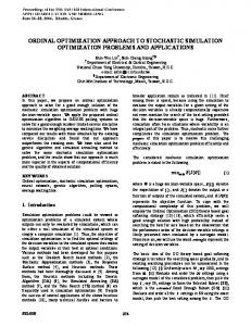
In the last decades, engineering design practices have experienced a paradigm shift, moving from the traditional build-and-test approach to more efficient, effective and versatile simulation-based design (SBD) methodologies. The integration of optimization algorithms with computer simulations has led to simulation-based design optimization (SBDO) procedures, with the aim of assisting and, if possible, guiding the designer in the the decision making process of complex engineering applications. The complexity of the systems along with the need of accurate performance analyses have led to the development and application of high-fidelity simulation codes, based on prime principles. Systems of partial differential equations are generally solved by computationally expensive black-box tools, such as those used in computational fluid dynamics (CFD) or structural finite element methods (FEM). The ever-increasing demand for accuracy and the complexity of structures and systems results to be more and more time consuming, in the simulation process. In several engineering fields, the evaluation of a single design can take as long as many days or even weeks. For this reason, new methods that can speed up the simulation time and the optimization process, saving time and money, are sought-after. SBD optimization procedures have been developed in order to integrate, efficiently and effectively, numerical simulations, design modification tools, and optimization algorithms (see Fig. 1). For this reason, SBDO is actually an essential part of the design of complex engineering systems since the conceptual and early design stages. Despite dramatic advances in computer hardware and software performance, the goal of fast, flexible and accurate simulation and optimization is yet to be achieved. Creating a system that has acceptable performance and provides useful results is a significant challenge. There are plenty of challenging real applications in sciences where optimization is naturally involved, and sophisticated minimization techniques are definitely necessary in order to allocate resources. SBD optimization for shape design has been widely applied to several engineering fields, such as aerospace [1, 2, 3, 4, 5], automotive [6, 7, 8, 9], structural [10, 11] and naval [12, 13, 14, 15, 16] engineering, where the shape design is of primary importance for the vehicle performance (e.g., aerodynamic, aeroelasticity, flight mechanics, hydrodynamics, seakeeping, structures, heat transfer). SBDO methodologies generally require large computational simulations to assess the performance of a design and evaluate the relative merit of design alternatives. In this context, an automated SBDO needs to integrate (i) simulation tools (for structures, fluids, etc.) and (ii) minimization algorithms with (iii) geometry modification and automatic meshing algorithms. To obtain an automated process this three fundamental elements have to be linked together in a robust, efficient, and effective way (see Fig. 1). Despite their importance, there are no satisfactory rules or guidelines for such issues. Obviously, the actual efficiency of an algorithm depends on many factors such as the inner working of an algorithm, the information needed (such as objective functions and their derivatives), and implementation details. The efficiency of a solver is even more complicated, depending on the actual numerical methods used and the complexity of the problem of interest. As for choosing the right algorithms for the right problems, there are many empirical observations, but no agreed guidelines. In fact, there is no universally efficient algorithms for all types of problems [17]. Therefore, the choice depends on several factors and is sometimes subject to the personal preferences of researchers and decision makers. Within SBDO, a nonconvex nonlinear programming problem is solved, where the objective function represents the performance of the engineering system under analysis and is usually of the black-box type, with values provided by computationally-expensive computer simulations. Up to 15-20 years ago, to a large extent, the main interest of theoreticians in optimization was for methods based on the use of derivatives. This was basically due to the following three strong reasons: - in several cases derivatives are available when solving computational problems. In particular, they are always ‘analytically’ available if the nonlinear functions involved are known in closed form [18]), and they can be exactly computed (not simply approximated) at reasonable cost in small-medium scale problems [19, 20]; 5

A. Serani

INTRODUCTION

Figure 1: Simulation-based design optimization framework - strong theoretical results have been developed, both in terms of convergence and computational performance, for optimization methods where derivatives (say of first/second order) are available; - the use of machine resources at a cheaper cost has allowed the solution of problems where derivatives can be suitably approximated by finite differences, using either coarse or fine techniques. On the other hand, engineering design offers a huge number of real-world problems where scientists are continuously asked to apply robust methods, using the most recent theoretical advances. In particular, design problems often include functions which are non-differentiable or where the use of derivatives is possibly discouraged. The following issues motivate the latter statement and give more precise guidelines for analyzing and improving optimization procedures not involving derivatives. • For ‘large scale’ problems, computing derivatives by finite differences might be prohibitively costly, and also Automatic Differentiation [18] might be of difficult application. Furthermore, the computation of derivatives by finite differences proved to be very harmful when the scale of the problem increases. Potential design improvements significantly depend on dimension and extension of the design space: high dimension and variability spaces are more difficult and expensive to explore but, at the same time, potentially allow for bigger improvements. • Most of the codes for complex design problems are ‘parameter dependent’, and the parameters need to be properly assessed. Their correct choice in practice implies that the overall performance of the code needs to be optimized with respect to those parameters. Thus, an implicit optimization problem with respect to these parameters requires a solution, and surely the derivatives of the functions involved are unavailable, being the output of a non-differentiable code. • Most of the design problems need solution procedures where expensive simulations are performed. Typically, simulations are affected by ‘noise’, systematic errors arise and stochastic parameters are used, so that derivatives are essentially unavailable or their use may lead to completely destroy the robustness of procedures [21]. The aforementioned issues contribute to motivate the use of efficient and effective derivative-free global methods, in order to solve a wide range of challenging problems. Derivative-free global optimization algorithms have been developed and effectively applied to SBD optimization, providing global approximate solutions to the design problem [22, 23, 24]. Moreover, shape optimization research has focused on shape and topology parameterizations, as a critical issue to achieve the desired level of design variability, and some recent research focused on research space variability and dimensionality reduction for efficient analysis and optimization procedures [5, 25].

6

A. Serani

INTRODUCTION

When global techniques are used with CPU-time expensive solvers, the optimization process is computationally expensive and its effectiveness and efficiency remain an algorithmic and technological challenge. Although complex SBD applications are often solved by metamodels [26, 27], their development and assessment require benchmark solutions, with simulations directly connected to the optimization algorithm. These solutions are achieved only if affordable and effective optimization algorithms are available. Several global optimization algorithm, such as simulated annealing (SA) [28, 29], particle swarm optimization (PSO) [30], ant colony optimization (ACO) [31], and genetic algorithms (GA) [32] have been deeply investigated in the last years [33, 34], and several new algorithms appeared recently, such as artificial fish-swarm algorithm (AFSA) [35], mesh adaptive direct search (MADS) [36, 37], firefly algorithm (FA) [38], cuckoo search (CS) [39], and bat algorithm (BA) [40]. Derivativefree global optimization approaches are often preferred to local approaches when objectives are non-convex and/or noisy, and when multiple local optima cannot be excluded, as often encountered in SBDO. Although global optimization approaches are a good compromise between exploration and exploitation of the research space, they could still get trapped in local minima and the convergence to a global minimum cannot be proven. If the research region to explore is known a priori, local optimization approaches can give an accurate approximation of the local minimum. Nevertheless, their convergence may be computationally expensive, and the information is usually not available a priori. For these reasons, the hybridization of global optimization algorithms with local search methods is an interesting research field, especially if CPU-time expensive black-box functions are involved, where the qualities of both methods can be efficiently and robustly coupled. It is worth noting that a large variety of derivative-free global and local methods available in the literature are stochastic/probabilistic. These methods make use of random coefficients and have been developed to the aim of sustaining the variety of the search for an optimum. This property implies that statistically significant results can be obtained only through extensive numerical campaigns. Such an approach can be too expensive (often almost unaffordable) in SBD optimization for industrial applications, when CPU-time expensive computer simulations are used directly as analysis tools. For this reason, deterministic approaches have been successfully developed and applied to SBD optimization. The objective of the present work is introduce, assess, and apply several optimization and geometry modification techniques for an efficient and effective use in the SBDO context. Chapter 1 introduce six derivative-free global and global/local optimization algorithms, suitable for an efficient and effective application in the SBDO context. Chapter 2 defines the three shape deformation methodologies used herein and the dimensionality reduction concept. The numerical solvers used for naval engineering application are presented in Chapter. 3. Chapter 4 presents the optimization algorithm parameters to be assess on seventy-three analytical test function, in order to define a useful guideline for each algorithm, and the naval engineering SBDO benchmark problem, used to verify and compare the algorithms performance. The results obtained on the test functions and the naval SBDO problems are presented and discussed in Chapter 5. Finally, Chapter 6 is devoted to the conclusions remark and the possible future work related to this thesis.

7

Chapter 1

Optimization algorithms “Begin at the beginning” the King said gravely, “and go on till you come to the end: then stop” — Lewis Carroll, Alice in Wonderland

Optimization problems can be formulated in several ways. optimization problem as Minimize fi (x), subject to h j (x) = 0, and to gk (x) ≤ 0,

The best-known formulation is to write a nonlinear i = 1, . . . , M j = 1, . . . , J k = 1, . . . , K

(1.1)

where fi , h j , and gk are general nonlinear functions. Here, the design vector x = [x1 , x2 , . . . , xN ]T can be continuous, discrete, or mixed in N-dimensional space. The functions fi are the objective or cost functions, whereas h j and gk are equality and inequality constraints, respectively. When M > 1, the optimization is multi-objective or multicriteria. It is possible to combine different objectives into a single objective, though multi-objective optimization can give far more information and insight into the problem. The present work deals only with single-objective optimization algorithm. Equation 1.1 represents in general a Non-deterministic polynomial-time hard (NP-hard) problem and no efficient (in the polynomial sense) solutions exist for a given problem. Thus, the challenges of research in computational optimization and applications are to find the most suitable algorithms for a given problem in order to obtain good solutions (perhaps also the best solutions globally), in a reasonable timescale with a limited amount of resources. An efficient optimizer is very important to ensure the optimal solutions are reachable. There are several optimization algorithms in the literature, and no single algorithm is suitable for all problems, as dictated by the No Free Lunch Theorems [17]. Optimization algorithms can be classified in many ways, depending on the characteristics that are compared. Algorithms can be classified as gradient-based (or derivative-based) and gradient-free (or derivative-free). The classic methods of steepest descent and the Gauss-Newton methods are gradient-based, as they use the derivative information in the algorithm, whereas the Nelder-Mead downhill simplex method [41] is a derivative-free method because it uses only the values of the objective, not any derivatives. Algorithms can also be classified as deterministic or stochastic. If an algorithm works in a mechanically deterministic manner without any random nature, it is called deterministic. For such an algorithm (i.e. downhill simplex methods), it will reach the same final solution if it starts with the same initial point. On the other hand, if there is some randomness in the algorithm, the algorithm will usually reach a different point every time it is run, even starting with the same initial point (i.e. genetic algorithms). This property implies that statistically significant results can be obtained only through extensive numerical campaigns. From the mobility point of view, algorithms can be classified as local or global. Local search algorithms typically converge toward a local optimum, not necessarily the global optimum, and such algorithms are often deterministic and have no ability of escaping local optima. On the other hand, the optimization procedure always try to find the global optimum for a given problem, and if this global optimality is robust, it is often the best, though it is not always possible to find such global optimality [42]. For global optimization [43], local search algorithms are usually not suitable. Modern metaheuristic algorithms, in most cases, are intended for global optimization. Although global optimization approaches are a good compromise between exploration and exploitation of the research space, they could still get trapped in local minima and the convergence to a global minimum cannot be

8

A. Serani

CHAPTER 1. OPTIMIZATION ALGORITHMS

proven. If the research region to explore is known a priori, local optimization approaches can give an accurate approximation of the local minimum, nevertheless, their convergence may be computationally expensive, and the information is usually not available a priori. Global/local hybrid algorithms tries to couple efficiently and robustly the qualities of both this methods. From the optimization point of view, the choice of the right optimizer or algorithm for a given problem is crucially important. The algorithm chosen for an optimization task will largely depend on the type of the problem, the nature of an algorithm, the desired quality of solutions, the available computing resource, the time limit, the availability of the algorithm implementation, and the expertise of the decision makers. The nature of an algorithm often determines if it is suitable for a particular type of problem. For example, gradient-based algorithms are not suitable for an optimization problem with a discontinuous objective. Generally, if the objective function of an optimization problem at hand is highly nonlinear and multimodal, gradient-based algorithm are inappropriate, whereas global optimizers are more suitable. This chapter provide a brief description of six single-objective deterministic derivative-free global and hybrid global/local optimization algorithm suitable for SBD global optimization problem in ship hydrodynamics. Two algorithms are well-known global optimization approaches, specifically a deterministic version of the particle swarm optimization method (DPSO) [44] and the DIviding RECTangles (DIRECT) algorithm [45]. Other three algorithms are hybrid global/local techniques integrated in DPSO and DIRECT enhancing the global methods with proved stationarity of the final solution; a hybrid DPSO coupled with line search-based derivative-free optimization (LS-DF PSO) [23], two hybrid DIRECT method coupled with line search-based derivative-free optimization (DIRMIN and DIRMIN-2) [24]. The last one is a novel metaheuristic based on the dynamics a fish shoal in search for food, namely the fish shoal algorithm (FSA) [46].

1.1

Particle Swarm Optimization algorithm

Particle Swarm Optimization (PSO) was originally introduced in Ref. [30], based on the social-behavior metaphor of a flock of birds or a swarm of bees searching for food. PSO belongs to the class of heuristic algorithms for single-objective evolutionary derivative-free global optimization. The original PSO makes use of random coefficients, aiming at sustaining the variety of the swarm’s dynamics. This property implies that statistically significant results can be obtained only through extensive numerical campaigns. Such an approach can be too expensive in SBD optimization for industrial applications, when CPUtime expensive (high-fidelity) computer simulations are used directly as analysis tools. For these reasons efficient deterministic approaches (such as deterministic PSO, DPSO) have been developed, and their effectiveness and efficiency in industrial applications in ship hydrodynamics problems have been shown, including comparisons with local methods [22] and random PSO [47]. Moreover, the availability of parallel architectures and high performance computing (HPC) systems has offered the opportunity to extend the original synchronous implementation of DPSO (S-DPSO) to CPU-time efficient asynchronous methods (A-DPSO) [48, 49].

1.1.1

PSO formulation

The original formulation of the PSO algorithm, as presented in [50], reads ( n (x n n n vn+1 = wvnj + c1 r1, j j j,pb − x j ) + c2 r2, j (xgb − x j ) n+1 n+1 n xj = xj +vj

(1.2)

The above equations update velocity and position of the j-th particle at the n-th iteration, where w is the inertia n and r n are uniformly distributed random numbers weight; c1 and c2 are the social and cognitive learning rate; r1, j 2, j in [0, 1]; x j,pb is the personal best position ever found by the j-th particle and xgb is global best position ever found considering all particles. An overall constriction factor χ is used in [51, 52, 53, 54, 55], instead of the inertia weight w. Accordingly, the system in Eq. 1.2 is recast in the following equivalent form h i ( n (x n n n vn+1 = χ vnj + c1 r1, j j j,pb − x j ) + c2 r2, j (xgb − x j ) (1.3) xn+1 = xnj + vn+1 j j In order to provide necessary (but possibly not sufficient) conditions which avoid divergence of particles trajectories, the following condition: χ=

2 q , √ 2−ϕ− ϕ 2 −4ϕ

where ϕ = c1 + c2 , ϕ > 4 (1.4)

9

A. Serani


is indicated in [52], where setting the value of ϕ to 4.1, with χ = 0.729, c1 = c2 = 1.494 is suggested. Note that PSO schemes including both the parameters w and χ have been also proposed in the literature.

1.1.2

DPSO formulation

In order to make PSO more efficient and repeatable for use within SBD, a deterministic version of the algorithm n = r n = 1 in Eq. 1.3, which become (DPSO) was formulated in [22] by setting r1, j 2, j h i ( vn+1 = χ vnj + c1 (x j,pb − xnj ) + c2 (xgb − xnj ) j (1.5) xn+1 = xnj + vn+1 j j In the context of SBD for ship design optimization, as mentioned before, the formulation of Eq. 1.5 was compared to the original in [47]. DPSO is therefore used for all the subsequent analyses. Using the above formulation, it is possible to prove that the necessary (but possibly not sufficient) conditions which ensure that the trajectory of each particle does not diverge [56], is ( 0 < |χ| < 1 (1.6) 0 < ω < 2 (χ + 1) where ω = χ(c1 + c2 ). Introducing β=

ω 2(χ + 1)

and assuming χ > 0 as usually in the literature, the conditions of Eq. 1.6 reduce to ( 0 Nmax return fmin , xmin

Here, U represents the unit hyper-cube, β is the tolerance used in the stopping criterion of the derivative-free local minimizations, γ is the activation trigger defining the starting point of the derivative-free local searches as ratio of the maximum number of function evaluation Nmax , and fml is the minimum value found by the derivativefree local searches. At each iteration n, every hyper-rectangle in Hn is characterized by the length of its diagonal and the value of the objective function at its centroid. Hence, provided that the Lipschitz constant is known, for every hyper-rectangle it is possible to compute a lower bound. An hyper-rectangle is declared potentially optimal (P n ) and then selected for further subdivision if an estimate L > 0 of the Lipschitz constant exists such that it yields the best estimated lower bound among all the hyper-rectangles. The subdivision performed in Step (9) is carried out by dividing the hyper-rectangles along the longest edges, thus guaranteeing that the hyper-rectangles shrink on every dimension in a sufficiently balanced way. The local minimizations at Step (4) are performed by using the derivative-free local optimization algorithm for bound constrained problems proposed in Ref. [75]. It performs derivative-free line searches along the coordinate directions. At every iteration, the maximum of the step-lengths gives a measure of stationarity of the current iterate (see e.g. [21]) and motivates the stopping criterion adopted at Step (4) of DIRMIN. As shown by [65], the DIRMIN algorithm can be efficient, in terms of function evaluations, with respect to the original DIRECT algorithm. The maximum number of function evaluations is used as stopping criterion of DIRMIN. It should be noted that the DIRECT algorithm is obtained from DIRMIN by simply replacing Step (4) with the assignment fml = +∞.

1.4.2

DIRMIN-2 formulation

DIRMIN-2 is a modification of DIRMIN. Rather than performing the derivative-free local minimizations starting from the centroids of all the potentially optimal hyper-rectangles P n , a single derivative-free local minimization is performed starting from the best point produced by dividing the potentially optimal hyper-rectangles. The derivative-free local optimization algorithm proposed in Ref. [75] is used. Details of DIRMIN-2 are given Alg. 6 15

A. Serani


Algorithm 6 DIRMIN-2 pseudo-code 1: 2: 3: 4: 5: 6: 7: 8: 9: 10: 11: 12: 13: 14:

Hn = {U}, with n = 0, c = center of U, fmin = f (c), xmin = {c}, β > 0, γ ∈ [0, 1], Nmax ≥ 0 repeat Set n = n + 1, identify the potentially optimal hyper-rectangles P n in Hn−1 and set fmold = fmin subdivide the potentially optimal hyper-rectangles to build Hn evaluate f at the centers of the new hyper-rectangles let c˜ ∈ arg min{ f (c) : c ∈ Cn }, where Cn the set of the centers of the hyper-rectangles Hn if function evaluations ≥ γ · Nmax then perform a local minimization starting from c˜ until the maximum step-length becomes smaller than the tolerance β , and let fml be the best function value found else set fml = +∞ end if fmin = min fmold , fml , min{ f (c) : c ∈ Cn } , xmin ∈ {x ∈ U : f (x) = fmin } until function evaluations > Nmax return fmin , xmin

Note that, when arg min{ f (c) : c ∈ Cn } is not a singleton, c˜ is the centroid of the first hyperectangle (among those produced at step 4) for which f (˜c) = min{ f (c) : c ∈ Cn }. The rationale behind the definition of DIRMIN-2 hinges on considering the subdivision of potentially optimal hyper-rectangles as a crude kind of local search, which can be improved by the use of a more sophisticated and efficient local minimization algorithm. Also in this case, the DIRECT algorithm is obtained from DIRMIN-2 by simply replacing Step (6) and (7) with the assignment fml = +∞.

1.5

Fish Shoal Algorithm

The fish shoal algorithm (FSA) is a deterministic derivative-free global optimization algorithm, introduced and developed in [46, 76], for solving engineering optimization problems with costly objective functions. The method is intended for unconstrained single-objective maximization and is based on a simplified social model of a fish shoal in search for food. FSA is formulated starting from the dynamics of a single individual belonging to a fish shoal in search for food, and subject to a shoal attraction force and a food-related attraction force. This formulation differentiates FSA from the artificial fish-swarm algorithm [77] and other metaheuristics such as PSO, for the direct use of the objective function value (food-related attraction force).

1.5.1

A brief overview of fish shoal behavior

In biology, fishes that stay in group for social reasons are shoaling. Shoaling offers numerous benefits to individual fish, including increased success in finding food, access to potential mates, and increased protection from predators. Fish shoals might be a group of mixed species and sizes that have gathered randomly near some local resource. Although shoaling fish can relate to each other in a loose way, with each fish swimming and foraging somewhat independently, they are nonetheless aware of the other members of the group as shown by the way they adjust behavior such as swimming, so as to remain close to the other fish in the group. If the shoal becomes more tightly organised, with the fish synchronising their swimming so they all move at the same speed and in the same direction in a coordinated manner, they are schooling. Shoaling fish can shift into a disciplined and coordinated school, then shift back to an amorphous shoal within seconds. Such shifts are triggered by changes of activity from feeding, resting, travelling or avoiding predators. Pitcher et al. [78], in their study of foraging behavior in shoaling cyprinids, have proven that swimming in groups enhances foraging success. In this study, the time it took for groups of minnows and goldfish to find a patch of food was quantified. The number of fishes in the groups was varied, and a statistically significant decrease in the amount of time necessary for larger groups to find food was established. This is directly related to the presence of many eyes searching for the food, because fishes in shoal share information by monitoring each others behavior closely. Feeding behavior in one fish quickly stimulates food-searching behavior in others [79]. Observations on the foraging behavior of captive golden shiner found they formed shoals, which were led by a small number of experienced individuals who knew when and where food was available [80]. If all golden shiners in a shoal have similar knowledge of food availability, there are few individuals that still emerge as natural leaders and behavioral tests suggest they are naturally bolder. Fish generally prefer larger shoals [81]. Larger shoals may find food

16

A. Serani


faster, though that food would have to be shared amongst more individuals. Competition may mean that hungry individuals might prefer smaller shoals or exhibit a less preference for very large shoals. Such foraging behavior of fish shoal can be formulated in such a way that it can be associated with the objective function to be optimized, and this makes possible to formulate novel optimization algorithms.

1.5.2

FSA formulation

Consider an optimization problem of the type Maximize f (x) subject to l ≤ x ≤ u

(1.12)

where f is the objective function, x ∈ RN is the variable vector D normalized into a unit hyper-cuber U, with lower and upper bounds equal to l and u respectively. Now consider a foraging shoal of individuals x j , exploring the research space with the aim of finding an approximate solution for problem in Eq. 1.12. The shoal is modelled as a dynamical system and the dynamics of the j-th individual depends on a shoal attraction force δ j (Fig. 1.4a), and a food-related attraction force ϕ j (Fig. 1.4b), as ϕj m¨x j + ξ x˙ j + kδδ j = hϕ where

(1.13)

Ns

δ j = − ∑ (xi − x j )

(1.14)

i=1

and

Ns

2∆ f (bi , x j ) e(bi , x j ) 1 + kbi − x j kα i=1

ϕj=∑ with ∆ f (bi , x j ) =

f (bi ) − f (x j ) , ρ

e=

bi − x j kbi − x j k

(1.15)

(1.16)

In the above equations, m, ξ , k and h ∈ R+ define the shoal dynamics; Ns ∈ N+ is the shoal size; α ∈ R+ tunes the food-related attraction force (see Fig. 1.4b); x j ∈ RN is the vector-valued position of the j-th individual; f (x) ∈ R is the objective function (representing the food distribution); bi is the best position ever visited by the i-th individual; ρ = f (b) − f (wn ) is a dynamic normalization term for f , with b the best position ever visited by the shoal and wn the worst position occupied by the shoal individuals at the current iteration n. Using the explicit Euler integration scheme, the FSA iteration become m

vn+1 − vnj j ∆t

ϕj = −ξ vnj − kδδ j + hϕ

(1.17)

∆t ϕj −ξ vnj − kδδ j + hϕ m

(1.18)

which yields vn+1 = vnj + j Setting m = 1 finally gives   vn+1 ϕ j) = (1 − ξ ∆t)vnj + ∆t(−kδδ j + hϕ j  xn+1 = xn + vn+1 ∆t j j j

(1.19)

where xnj and vnj represent the individual position and velocity vector of the j-th individual at the n-th iteration, respectively.

17

CHAPTER 1. OPTIMIZATION ALGORITHMS 1

1

0.8

0.8

0.6

0.6 ϕj [-]

|δj| [-]

A. Serani

0.4

0.4 α=0.5

0.2

0.2

0

0

α=1.0 α=2.0

0

0.2

0.4 0.6 ||xi - xj|| [-]

0.8

1

0

0.2

0.4 0.6 ||bi - xj|| [-]

0.8

1

(a) (b) Figure 1.4: Shoal (a) and food-related (b) attraction forces, for Ns = 2 and ∆ f = 1 In Eq. 1.19, the integration step ∆t must guarantee the stability of the explicit Euler scheme, at least for the free dynamics. To this aim, consider the free dynamics of the k-th component of x (or k-th variable), say a. Consider the dynamics of a for the j-th individual a¨ j + ξ a˙ j + kδ j = 0

(1.20)

and finally for the entire shoal

where

    K = −k   

a˙ c˙

=

0 I −K −G

a c

=A

Ns − 1 −1 .. .

−1 Ns − 1 .. .

−1 −1 .. .

··· ··· .. .

−1 −1 .. .

−1 −1

··· ···

−1 −1

Ns − 1 −1

−1 Ns − 1

a c

(1.21)

    ,  

G = ξI

(1.22)

and I is the [Ns × Ns ] identity matrix. The solution of Eq. 1.21 is stable if Re(λ ) ≤ 0

(1.23)

where λ = −γ ± iω are eigenvalues of A. This yields 2γ ∆t ≤ 2 = ∆tmax γ + ω 2 min

(1.24)

Equation 1.19 represents a fully informed formulation, where each individual knows the story of the whole shoal. The FSA pseudo-code is shown in Alg. 7. Algorithm 7 FSA pseudo-code 1: 2: 3: 4: 5: 6: 7: 8: 9: 10: 11:

Normalize x into a unit hypercube U Initialize a shoal of Ns individuals Evaluate the ∆tmax by the linear system’s eigenvalues (Eq. 1.21) while n < Max number of iterations do for j = 1, Ns do Evaluate f (x j ) end for Update x jb , f (x jb ) and the attraction forces Update vn+1 and xn+1 j j end while Output the best solution found

18

Chapter 2

Shape design modification “I – I hardly know, sir, just at present – at least I know who I WAS when I got up this morning, but I think I must have been changed several times since then.” — Lewis Carroll, Alice in Wonderland

Shape design optimization finds the optimum shape for a given structural layout [82]. Obviously, the choice of the shape parametrization technique has a large impact on the practical implementation and often also on the success of the optimization process. Shape deformation methods have been an area of continuous and extensive research within the fields of computer graphics and geometry modelling. Consequently, a wide variety of techniques has been proposed during recent years [83]. The parametrization techniques can be divided into the following categories [82]: basis vector, domain element, partial different equation, discrete, polynomial and spline, CAD-based, analytical, and free-form deformation (FFD). In the context of SBDO, to be successful, the parametrization model must yield a compact and effective set of design variables so the solution time would be feasible. As a general statement it can be said that, in principle, the number (and the type) of parameters implicitly defines the diversity of the admissible shapes: since the larger the variety of potential designs, the larger the improvements it can be hope to find (starting from the original design), the importance of a proper choice of the design parameters is evident [84]. Starting from an initial design, so that all the details of the original shape are known, the adaptation of an existing surface/volumetric simulation grid according to an updated CAD geometry is a key component for performing the optimization in a fully automatic procedure. The importance of such a component further increase when dealing with complex geometry that prohibit automatic mesh generation or when using population-based optimization algorithm, i.e. evolutionary algorithm, which typically require the creation and evaluation of a large number of design variations in order to find a feasible solution [85]. Another issue that has to be addressed is that the computational grid adopted in the analysis must be regenerated or deformed each time there is the need to evaluate a new perturbed design, and this operation has to be performed in background, without any guarantee about the quality of the new mesh. When this has to be done in conjunction with CFD solvers, the regridding issues may become extremely relevant to the performance and the final result of the optimization [84]. In order to avoid the costly mesh generation process for each design variation created during the optimization, one typically aims at adapting an initial simulation mesh alongside with the surface. A type of deformation methods that naturally fulfils the above requirements are so-called space deformations. Deformation (more than regeneration) of the computational grid represents a good approach to the problem: (1) one doesn’t need to regenerate the whole volume grid each time the hull shape is perturbed, (2) the initial hull shape is preserved and (3) one can deform some part of the hull with a prescribed degree of continuity. The fundamental idea behind these methods is to deform the embedding space around an object, thereby deforming the object implicitly. From a mathematical point of view a space deformation is a function δ s : R3 −→ R3

(2.1)

that maps each point in space to a certain displacement. Given a deformation function, a geometry G can be transformed to a deformed geometry G 0 by computing updated point locations x0 = x + δ s (x)

19

(2.2)

A. Serani

CHAPTER 2. SHAPE DESIGN MODIFICATION

for each original point x ∈ G [83]. The following subsections show three different shape modification technique used in the present work, that satisfied the requirements described above. Specifically, free-form deformation (FFD), and orthogonal expansion over 2D and 3D subdomains are presented and described for using in simulation-based shape design optimization in naval engineering. Finally, since the use of the present (and also other) techniques allows the use of a possibly infinite number of variables causing an increase in the optimization costs, a design-space dimensionality reduction technique based on generalized Karhunen-Loève expansion [16, 86] is presented, in order to define a more effective and efficient (from the optimization point of view) design modification space.

2.1

Free-form deformation

Free-form deformation (FFD) is a geometry deformation technique used to model simple deformations of rigid objects, widely used in both academia and industry for SBDO [16, 47, 84, 87]. The technique was first described in [88], and is based on an earlier technique described in [89]. It is based on the idea of embedding an object to be deformed within a parallelepiped/cube lattice (see Fig. 2.1) or another shell object, and transforming the object within the cube as the lattice is deformed. Deformation of the lattice is based on the concept of so-called hyper-patches, which are three-dimensional analogues of parametric curves such as Bézier curves, B-Splines, or NURBS (Non Uniform Rational Basis-Splines). The deformation procedure can be divided in several step: (1) a control lattice point has to be generated and adapted to the deformation scenario, (2) the local coordinates with respect to the control lattice have to be computed for each point to be deformed, (3) express each object point x ∈ G as a linear combination of lattice control points ci jk and basis function Bi so that l

m

x=∑ ∑

n

∑ ci jk Bi (u)B j (v)Bk (w)

(2.3)

i=0 j=0 k=0

where (u, v, w) are the local coordinates of x with respect to the control lattice, and l, m, n are the numbers of control points in each direction. Defining u(x) := (u, v, w),

B p (u(x)) := Bi (u)B j (v)Bk (w)

(2.4)

as well as δ c p := δ ci jk = c0i jk − ci jk where

c0i jk

(2.5)

denotes an updated control point location, the FFD space deformation function can be expressed by δ s (x) = ∑ δ c p B p (u(x))

(2.6)

p

Finally, the deformation is performed by moving the control point and computing the updated object point locations.

Figure 2.1: Example of FFD parallelepiped lattice on the Delft catamaran demi-hull [16] The FFD formulation is independent of grid topology and that independence makes it suitable for a variety of analysis codes, such as low- and high-fidelity analysis tool. On the other hand, the FFD variables may have little or no physical significance for the design engineers, thereby making it difficult to establish an effective and compact set of design variables. 20

A. Serani

2.2


Orthogonal basis functions expansion over 2D subdomains

An effective and efficient shape design modification method in the context of SBDO is introduced in [90]. The shape deformation is performed by the superposition, on the original shape/grid, of bi-dimensional orthogonal basis functions expansion (OBFE 2D). The orthogonal basis functions are linearly independent and are directly defined on the curvilinear coordinates ξ and η of the object (computational grid) ψ i (ξ , η) : G = [0, Lξ ] × [0, Lη ] ∈ R2 −→ R3 , as

i = 1, ..., N

(2.7)

N

δ s (ξ , η) = ∑ αi ψ i (ξ , η)

(2.8)

i=1

where the coefficients αi ∈ R (i = 1, . . . , N) are the design variables, ri πξ ti πη ψ i (ξ , η) := sin + φi sin + χi eq(i) Lξ Lη

(2.9)

and the following orthogonality property is imposed: ZZ G

ψ i (ξ , η) · ψ j (ξ , η)dξ dη = δi j

(2.10)

In Eq. 2.9, ri and ti ∈ R define the order of the function in ξ and η direction respectively; φi and χi ∈ R are the corresponding spatial phases; Lξ and Lη ∈ R define the domain size; eq(i) is a unit vector, so that the design modifications may be applied in x, y or z direction, with q(i) = 1, 2, or 3 respectively. An example of OBFE 2D is shown in Fig. 2.2. 1

1

0.8

1 0.8

0.5

0 0.4

-0.5

0.2

0.2

0.4

0.6

0.8

1

00

-0.5

0.2

0.4

ξ

0.6

0.8

1

1

-1

00

0.2

0.4

0.8

1

-0.5

0.6

0.8

1

-1

ξ

0

0 0.4

-0.5

0.2 00

0.2

0.4

0.6

0.8

1

-1

(ri = 1, φi = 0, ti = 3, χi = 0)

-0.5

0.2 00

ξ

(ri = 1, φi = 0, ti = 2, χi = 0)

0.5

0.6

0.4

0.2

1

η

η

0

-1

0.8

0.6

0.4

1

1

0.5

η

0.6

0.8

(ri = 4, φi = 0, ti = 1, χi = 0) 1

0.8

0.5

0.6

ξ

(ri = 3, φi = 0, ti = 1, χi = 0) 1

0.4

-0.5

0.2

ξ

(ri = 2, φi = 0, ti = 1, χi = 0)

0.2

0 0.4

0.2

-1

0.5

0.6

η

η

0

1

0.8

0.6

0.4

00

1

0.5

η

0.6

00

1

0.2

0.4

0.6

0.8

1

-1

ξ

(ri = 1, φi = 0, ti = 4, χi = 0)

Figure 2.2: Example of 2D orthogonal functions ψ i (ξ , η) This kind of technique can be applied on the whole object or a part of it, and the OBFE 2D design variables can be related to a physical meaning, e.g. Fig. 2.2a shows the movement of volumes from a side to another of the object conditional to the zone of application and the direction of the patch. On the other hand, the limit of this approach is in the direct use of the curvilinear coordinates corresponding to the object grid: the same orthogonal function corresponds to different shape modifications, dependently to grid discretization.

21

A. Serani

2.3


Orthogonal basis functions expansion over 3D subdomains

The OBFE 2D method has been extended to three-dimensional orthogonal basis functions expansion (OBFE 3D) [91], to release the shape modification method from the computational grid topology and to be more effective and efficient in the context of SBDO. The shape deformation is performed by the superposition, on the original shape/grid, of OBFE 3D defined on the Cartesian coordinates x, y, z over a hyper-rectangle ϕ i (x, y, z) : G = [0, Lx ] × [0, Ly ] × [0, Lz ] ∈ R3 −→ R3 , as

i = 1, ..., N

(2.11)

N

δ s (x, y, z) = ∑ βi ϕ i (x, y, z)

(2.12)

i=1

where the coefficients βi ∈ R (i = 1, . . . , N) are the design variables, mi πy li πz ni πx ϕ i (x, y, z) := sin + φi sin + χi sin + θi eq(i) Lx Ly Lz

(2.13)

and the following orthogonality property is imposed: ZZZ G

ϕ i (x, y, z) · ϕ j (x, y, z)dxdydz = δi j

(2.14)

In Eq. 2.13, ni , mi and li ∈ R define the order of the function in x, y and z direction respectively; φi , χi and θi ∈ R are the corresponding spatial phases; Lx , Ly and Lz ∈ R define the hyper-rectangle dimensions; eq(i) is a unit vector. Modifications may be applied in x, y or z direction, with q(i) = 1, 2, or 3 respectively. This kind of method can be applied on the whole object or a part of it, and it is independent of grid topology. On the other hand, there isn’t a direct physical meaning of the object surface modification because the OBFE 3D are non linear on the object surface.

2.4

Automatic grid modification

The shape modification, performed by the techniques previously presented, can be directly reflected in the body surface grid deformation, for this reason they are also suitable in the optimization problems involving solvers that need only a surface grid (e.g. potential flow). On the contrary, when the optimization problem involves volume grid solvers (e.g. RANS or FEM), the surface grid modifications need to be transposed also to the volume grid: the methodology used in the present work is presented in the following.

2.4.1

Volume grid modification

The volume grid (e.g. boundary layer grid) is automatically modified, in order to reflect the shape modification applied to the the body (surface) grid. Assume that the body surface grid is defined with index J = 1 and spanned by indices I = 1, . . . , Imax and K = 1, . . . , Kmax . Accordingly, the volume grid is spanned by I = 1, . . . , Imax , J = 1, . . . , Jmax , and K = 1, . . . , Kmax , with J = Jmax corresponding to the outer surface. Once the grid nodes of the body surface at J = 1 are modified following the shape modification vector δ s (e.g. defined by FFD, OBFE 2D, or OBFE 3D), any arbitrary inner node of the volume grid (J = 2, . . . , Jmax − 1) is modified similarly to Eq. 2.2, as x = x0 + δ

(2.15)

with

l∗ − l l δ s + ∗ δ ∗s (2.16) l∗ l where l is the distance between (original) inner and body surface nodes, with arbitrary J and J = 1 respectively (and same I and K indices); l ∗ is the distance between (original) outer and body surface nodes, with J = Jmax and J = 1 respectively (and same I and K indices); δ ∗s is the modification of the outer surface (J = Jmax ): δ=

δ ∗s = c δ s

(2.17)

with c ∈ R+ 0. ¯ The distance l (and l ∗ ) may be evaluated in the simplest form as the Euclidean distance l: l = l¯ = kx0 − xs,0 k 22

(2.18)

A. Serani


Alternatively, the approximate curvilinear distance lˆ along the grid line at constant I and K may be used [92]: J−1

l = lˆ =

( j+1)

∑ kx0

( j)

− x0 k

(2.19)

j=1

where superscripts indicate grid indices, limited to J for the sake of compactness (since I and K are constant).

2.5

Design-space dimensionality reduction by generalized Karhunen-Loève expansion

Shape optimization research has focused on shape and topology parameterizations, as a critical issue to achieve the desired level of design variability [93, 94, 95]. Some recent research focused on research space variability and dimensionality reduction for efficient analysis and optimization procedures [5, 25]. A quantitative approach based on the Karhunen-Loève expansion (KLE, also known as proper orthogonal decomposition, POD) has been formulated for a pre-optimization assessment of the shape modification variability (see the left box of Fig. 2.3) and the definition of a reduced-dimensionality global model of the design space [16, 96, 97]. The mathematical properties of the dimensionality-reduction by KLE are described in the following. Pre-optimization design space dimensionality reduction

Single/multi-disciplinary shape optimization loop Shape modification and automatic meshing

KLE-based dimensionality reduction

Shape modification tool

Single/multidisciplinary analysis (CFD, FEM, etc.)

Optimization algorithm

Figure 2.3: Scheme for single/multi-disciplinary shape optimization, including pre-optimization design-space dimensionality reduction Consider a geometric domain of interest G, which identifies the initial shape, and a set of coordinates x ∈ G. Assume that u ∈ U is the design variable vector, which defines a shape modification vector δ s . Consider the vector space of all possible square-integrable modifications of the initial shape, δ s (x, u) ∈ Lρ2 (G), where Lρ2 (G) is the Hilbert space defined by a generalized inner product Z

(f, g)ρ =

ρ(x)f(x) · g(x)dx

(2.20)

G

1

with associated norm kfkρ = (f, f)ρ2 , where ρ(x) ∈ R is a weight function. Generally, x ∈ Rm with m = 1, 2, 3, u ∈ RN with N number of design variables, and δ s ∈ Rl with l = 1, 2, 3 (with l not necessarily equal to m). Consider the design vector u as belonging to a stochastic space S with associated probability density function f (u). The associated mean shape modification is evaluated as hδδ s i =

Z U

ρ(x)δδ s (x, u) f (u)du

whereas the variance associated to the shape modification vector (geometric variance) is defined as E Z Z D σ 2 = kδˆ s k2 = ρ(x)δˆ s (x, u) · δˆ s (x, u) f (u)dxdu U

(2.21)

(2.22)

G

where δˆ s = δ s − hδδ s i, and h·i denotes the ensemble average over u ∈ S. If the design shape is defined such that the mean shape corresponds to the original design, then hδδ s i = 0, ∀x, and therefore δˆ s = δ s . The aim of the KLE is to find an optimal basis of orthonormal functions, for the linear representation of the deviation from the mean shape modification vector, expressed by δˆ s (x, u) =

∞

Φk (x)dx ∑ αk (u)Φ k=1

23

(2.23)

A. Serani


‫܍‬ଶ ȳ

‫܍‬ଵ

ऑԢ

!઻ሺ‫ݔ‬ǡ ‫ܝ‬ሻ ‫ ݔ‬

ऑ

Figure 2.4: Scheme and notation for the current formulation, showing an example for m = 1 and l = 2. where αk (x) = (δˆ s , Φ k )ρ =

Z G

ρ(x)δˆ s (x, u) · Φ k (x)dx

(2.24)

are the basis-functions component, used hereafter as new design variables. The optimality condition associated to the KLE refers to the geometric variance retained by the basis functions through Eq. 2.23. Combining Eqs. 2.22–2.24 yields σ2 =

∞

∞

∞

Φk , Φ j )ρ = αk α j (Φ

∑∑

k=1 j=1

∑

2 αj =

j=1

∞

∑

D E (δˆ , Φ j )2 ρ

(2.25)

j=1

The basis retaining the maximum variance is so formed by those Φ that are solutions of the variational problem D E Φ) = (δˆ s , Φ j )2ρ maxΦ ∈Lρ2 (G ) J(Φ (2.26) Φ, Φ )2ρ = 1 subject to (Φ which yields to Φ(x) = LΦ

Z G

D E ρ(y) δˆ s (x, u) ⊗ δˆ s (y, u) Φ (y)dy = λ Φ (x)

(2.27)

where L is the selfadjoint integral operator whose eigensolutions define the optimal basis functions for the linear Φ k }∞ representation of Eq. 2.23. Therefore, its eigenfunctions (KL modes) {Φ k=1 are orthogonal and form a complete 2 basis for Lρ (G). Additionally, it may be proven [16] that σ2 =

∞

∑ λj

(2.28)

j=1

where the eigenvalues λ j (KL values) represent the variance retained by the associated basis function Φ j , through its component α j in Eq. 2.23. Φ k }∞ Finally, the solutions {Φ k=1 of Eq. 2.27 are used to build a reduced-dimensionality space for the shape modification. Assume that n, with 0 < n ≤ 1, is the desired level of confidence for the shape modification variability, Eq. 2.23 may be truncated to the N-th order, provided that N

∞

∑ λk ≥ n ∑ λk = nσ 2 k=1

k=1

with λk ≥ λk+1 . Details of equations and numerical implementations are given in Ref. [16].

24

(2.29)

Chapter 3

Hydrodynamic solvers “Contrariwise,” continued Tweedledee, “if it was so, it might be; and if it were so, it would be; but as it isn’t, it ain’t. That’s logic.” — Lewis Carroll, Alice in Wonderland

The prediction of ship hydrodynamics performance can be broken down into three general areas: (1) resistance and propulsion, (2) seakeeping, and (3) manoeuvring. There are several basic approaches to predict the hydrodynamics performance of a vessel, and they can be classified as: empirical/statistical, experimental (either in modelor full-scale), and numerical (either rather analytical or using computational fluid dynamics (CFD)). In the simulation-based design optimization context, the “simulation” role is performed by the numerical approaches, specifically by low- and high-fidelity CFD solvers. For ship resistance, CFD has become increasingly important and is now an indispensable part of the design process. Typically inviscid free-surface methods based on the boundary element approach are used to analyse the forebody, especially the interaction of bulbous bow and forward shoulder. Viscous flow codes focus on the aftbody or appendages. Flow codes modeling both viscosity and the wave-making are widely applied for flows involving breaking waves. So far CFD has been used to gain insight into local flow details and derive recommendation on how to improve a given design or select a most promising candidate design for model testing [98]. For seakeeping, simple strip methods are used to analyze the seakeeping properties. These usually employ boundary element methods to solve a succession of two-dimensional problems and integrate the results into a quasi-three-dimensional result with usually good accuracy. Although a model of the final ship design is still tested in a towing tank, the testing sequence and content have changed significantly over time. Traditionally, unless the new ship design was close to an experimental series or a known parent ship, the design process incorporated many model tests. The process has been one of design, test, redesign, test, etc., sometimes involving more than ten models, each with slight variations. This is no longer feasible due to time-to-market requirements from shipowners and no longer necessary thanks to CFD developments. Combining CAD (computer-aided design) to generate new hull shapes in concert with CFD to analyze these hull shapes allows for rapid design explorations without model testing. With massive parallel computing and progress in optimization strategies, formal optimization of hulls, propellers, and appendages has drifted into industrial applications. CFD is increasingly used for the actual design of hull and propellers. Then often only the final design is actually tested to validate the intended performance features and to get a power prediction accepted in practice as highly accurate. As a consequence of this practice, model tests for shipyard customers have declined considerably since the 1980s. This was partially compensated for by more sophisticated and detailed tests funded from research projects to validate and calibrate CFD methods.

3.1

Fluid mechanics equations

For the velocities involved in ship flows, water can be regarded as incompressible, i.e. the density ρ is constant. Therefore we will limit ourselves here to incompressible flows. All equations are given in a Cartesian coordinate system with z pointing downwards. The continuity equation states that any amount flowing into a control volume also flows out of the control volume at the same time. Consider an infinitely small control volume (see Fig. 3.1) for the two-dimensional case, where u and v are the velocity components in x and y direction, respectively. The indices denote partial derivatives, e.g. ux = ∂ u/∂ x. Positive mass flux leaves the control volume; negative mass 25

A. Serani

CHAPTER 3. HYDRODYNAMIC SOLVERS

Figure 3.1: Control volume to derive continuity equation in two dimensions flux enters the control volume. The total mass flux has to fulfill: −ρdy u + ρdy(u + ux dx) − ρdx v + ρdx(v + vy dy) = 0

(3.1)

ux + vy = 0

(3.2)

The continuity equation in three dimensions can be derived correspondingly to: ux + vy + wz = 0

(3.3)

where w is the velocity component in z direction. The Navier–Stokes equations together with the continuity equation suffice to describe all real flow physics for ship flows. The Navier–Stokes equations describe conservation of momentum in the flow: ρ(ut + uux + vuy + wuz ) = ρ f1 − px + µ(uxx + uyy + uzz ) ρ(vt + uvx + vvy + wvz ) = ρ f2 − py + µ(vxx + vyy + vzz ) ρ(wt + uwx + vwy + wwz ) = ρ f3 − pz + µ(wxx + wyy + wzz )

(3.4)

where fi is an acceleration due to a volumetric force, p the pressure, µ the viscosity, and t the time. Often the volumetric forces are neglected, but gravity can be included by setting f3 =g. The left hand side of the Navier–Stokes equations without the time derivative describes convection, the time derivative describes the rate of change (source term), the last term on the right hand side describes diffusion. The Navier–Stokes equations in the above form contain on the light hand side products of the velocities and their derivatives. This is a nonconservative formulation of the Navier–Stokes equations. A conservative formulation contains unknown functions (here velocities) only as first derivatives. Using the product rule for differentiation and the continuity equation (Eq. 3.3), the non-conservative formulation can be transformed into a conservative formulation, e.g. for the first of the Navier–Stokes equations above: (u2 )x + (uv)y + (uw)z = 2uux + uy v + uvy + uz w + uwz = uux + vuy + wuz + u(ux + vy + wz ) = uux + vuy + wuz

(3.5)

Navier–Stokes equations and the continuity equation form a system of coupled, nonlinear partial differential equations. An analytical solution of this system is impossible for ship flows. Even if the influence of the free surface (waves) is neglected, todays computers are not powerful enough to allow a numerical solution either. Even if such a solution may become feasible in the future, it is questionable if it is really necessary for engineering purposes in naval architecture. Velocities and pressure may be divided into a time average and a fluctuation part to bring the Navier–Stokes equations closer to a form where a numerical solution is possible. Time averaging yields the Reynolds-averaged Navier–Stokes (RANS) equations, therefore u, v, w, and p are from now on time averages, whereas u0 , v0 , and w0 denote the fluctuation parts. For unsteady flows, high-frequency fluctuations are averaged over a chosen time interval (assembly average). This time interval is small compared to the global motions, but large compared to the turbulent fluctuations. Most computations for ship flows are limited to steady flows where the terms ut , vt , and wt vanish. The RANS equations have a similar form to the Navier–Stokes equations: ρ(ut + uux + vuy + wuz ) = ρ f1 − px + µ(uxx + uyy + uzz ) − ρ((u0 u0 )x + (u0 v0 )y + (u0 w0 )z ) ρ(vt + uvx + vvy + wvz ) = ρ f2 − py + µ(vxx + vyy + vzz ) − ρ((u0 v0 )x + (v0 v0 )y + (v0 w0 )z ) ρ(wt + uwx + vwy + wwz ) = ρ f3 − pz + µ(wxx + wyy + wzz ) − ρ((u0 w0 )x + (v0 w0 )y + (w0 w0 )z ) 26

(3.6)

A. Serani


including the derivatives of the Reynolds stresses (last term on the right hand side of Eq. 3.6). The time averaging eliminated the turbulent fluctuations in all terms except the Reynolds stresses. The RANS equations require a turbulence model that couples the Reynolds stresses to the average velocities. Neglecting viscosity and all turbulence effects turns the RANS equations into the Euler equations, which still have to be solved together with the continuity equations: ρ(ut + uux + vuy + wuz ) = ρ f1 − px ρ(vt + uvx + vvy + wvz ) = ρ f2 − py ρ(wt + uwx + vwy + wwz ) = ρ f3 − pz

(3.7)

Euler solvers allow coarser grids and are numerically more robust than RANS solvers. They are suited for computation of flows about lifting surfaces (foils) and are thus popular in aerospace applications. They are not so well suited for ship flows and generally not recommended because they combine the disadvantages of RANS and Laplace solvers without being able to realize their major advantages: programming is almost as complicated as for RANS solvers, but the physical model offers hardly any improvements over simple potential flow codes (Laplace solvers) [98]. A further simplification is the assumption of irrotational flow: ∇×v = 0

(3.8)

A flow that is irrotational, inviscid and incompressible is called potential flow. In potential flows the components of the velocity vector are no longer independent from each other. They are coupled by the potential φ . The derivative of the potential in arbitrary direction gives the velocity component in this direction: v = ∇φ

(3.9)

Three unknowns (the velocity components) are thus reduced to one unknown (the potential). This leads to a considerable simplification of the computation. The continuity equation simplifies to Laplaces equation for potential flow: ∆φ = φxx + φyy + φzz = 0 If the volumetric forces are limited to gravity forces, the Euler equations can be written as: p 1 2 =0 ∇ φt + (∇φ ) − gz + 2 ρ

(3.10)

(3.11)

Integration gives Bernoullis equation: 1 p φt + (∇φ )2 − gz + = const. 2 ρ

(3.12)

The Laplace equation is sufficient to solve for the unknown velocities. The Laplace equation is linear. This offers the big advantage of combining elementary solutions (so-called sources, sinks, dipoles, vortices) to arbitrarily complex solutions. Potential flow (PF) codes are still largely used tools in ship and propeller design.

3.2

Hydrodynamic tools

In the present work, the simulation-based design optimization problems, used as benchmark to test and assess the performance of the optimization algorithm, pertain the hull-form optimization for calm-water resistance reduction and improved seakeeping performance of two different kind of vessels. The analysis tools used both low- and high-fidelity solvers, and they are briefly introduced in the following subsections.

3.2.1

WAve Resistance Program

The WAve Resistance Program (WARP) is a code developed at CNR-INSEAN. The mathematical model is approximated by a Boundary Element Method, in which the integral equation on the boundary is approximated by a piecewise constant distribution of source density on quadrilateral plane panels. Wave resistance computations are based on the linear PF theory [99]. The simplest linear formulation (Kelvin linearization) is obtained by assuming ˜ that the actual flow is slightly perturbed from the free stream, and its potential function is given by φ = Ux + ϕ, which provides the Neumann-Kelvin (NK) problem for the Laplace equation. A further linearization, suggested 27

A. Serani


by Dawson [100], is based on the assumption that the flow near the body is perturbed around the double model ˜ NK is usually reasonable for slender bodies (DM) flow, and its potential function is given by φ = Ux + ϕd + ϕ. and high speeds, whereas DM is usually more suitable for wider bodies and low speeds. The wave resistance can be evaluated by both a pressure integral over the body surface and the transverse wave cut method [101], whereas the frictional resistance is estimated using a flat-plate approximation, based on the local Reynolds number [102]. The steady 2DOF (sinkage and trim) equilibrium is achieved by iteration of the flow solver and the body equation of motion.

3.2.2

Ship Motion Program

The Standard Ship Motion program (SMP) was developed at the David Taylor Naval Ship Research and Development Center in 1981, as a prediction tool for use in the Navys ship design process. SMP is a potential flow code based on linearized strip theory. It provides a predictions of the motions, i.e., displacements, velocities, and accelerations, for a ship advancing at constant speed, with arbitrary heading in both regular waves and irregular seas. The irregular seas are modelled using a two-parameter Bretschneider wave spectral model. Both long-crested and short-crested results are provided. In addition to the 6DOF responses, the absolute motion, velocity, acceleration, as well as the relative motion and velocity for various locations on the ship can also be obtained. The probabilities and frequencies of submergence, emergence, and/or slamming occurrence for various locations on the ship, are also available. Vertical shears and bending moments due to the ship motions can be produced [103].

3.2.3

CFDShip-Iowa

CFDShip-Iowa is a general-purpose unsteady Reynolds-averaged Navier-Stokes (URANS) CFD code that has been developed at the University of Iowa, IIHR-Hydroscience & Engineering, over the past 25 years, to handle a broad range of ship hydrodynamics problems. Originally designed to support both thesis and project research in the areas of resistance and propulsion, it has been successfully transitioned to Navy and university laboratories and industry, and has recently been extended to unsteady applications such as seakeeping and maneuvering. It was developed following a modern software-development philosophy, which was based upon open source, revision control, modular coding using Fortran 90/95, liberal use of comments, and an easy to understand architecture that enables model development by users. The equations are solved in an inertial coordinate system, either fixed to a ship or other frame moving at constant speed or in the earth system. The free surface is modelled with a single-phase capturing approach, which means that only the water flow is solved, enforcing kinematic and dynamic free surface boundary conditions on the interface. Arbitrary free surface topologies can be predicted, with the limitation that pressurized closed air/water packets (bubbles) cannot be simulated. It uses structured multiblock grids, and has overset capabilities. Capabilities include 6DOF motions, several turbulence models, moving control surface, multi-objects, advanced controllers, propulsion models, incoming waves and wind, bubbly flow, and fluid-structure interaction. Details of equations, numerical implementations and validation of the numerical solver are given in [104].

28

Chapter 4

Optimization problems “The time has come,” the walrus said,“to talk of many things: Of shoes and ships - and sealing wax - of cabbages and kings” — Lewis Carroll, Alice in Wonderland

4.1

Analytical test functions

A benchmark of seventy-three well-known analytical test functions [24, 44, 65, 105, 106, 107], including simple unimodal (i.e., those denoted by a superscript “*” in Tab. 4.1), highly complex multimodal, and not differentiable problems, has been used in order to assess the algorithms performance. Table 4.1 summarizes the test functions used herein, and the algorithm applied on each one. The analytical expressions of the test functions are reported in Appendix A. In the following, DPSO, LS-DF PSO, DIRMIN, DIRMIN-2, and FSA setting parameters are presented and discussed. The different setups have been used to verify and assess the algorithm performances. The results are presented in the next chapter.

4.1.1

DPSO setting parameters

The effectiveness and efficiency of DPSO for box constrained optimization are significantly influenced by four main setting parameters: (a) the number of swarm particles interacting during the optimization, (b) the initialization of the particles in terms of initial location and velocity, (c) the set of coefficients defining the personal or social behavior of the swarm dynamics, and (d) the method to handle the box constraints. These parameters and their effects on PSO have been studied by a number of authors [33, 50, 59] and a preliminary assessment of the performances of DPSO, varying (a), (b) and (c), is presented in Ref. [44]. In order to identify of the most effective and efficient parameters for both synchronous and asynchronous deterministic particle swarm optimization (S-DPSO and A-DPSO), for their use in SBD procedures, the DPSO parameters are defined in the following, and applied on 60 test functions (see Tab. 4.1), with dimensionality ranging from two to twenty. Their full-factorial combination is considered, resulting in a total of 420 DPSO setups. The simulation budget (maximum number of objective function evaluations) is studied up to 4096 times the number of variables. Number of particles The number of particles used (N p ) is defined as N p = 2m N ,

with m ∈ N [1, 7]

therefore ranging from 2N to 128N, where N is the number of design variables.

29

(4.1)

A. Serani

CHAPTER 4. OPTIMIZATION PROBLEMS

Table 4.1: Analytical test functions fp

Name

N

DPSO

LS-DF PSO

DIRECT

DIRMIN

DIRMIN-2

FSA

f1 f2 f3 f4 f5 f6 f7 f8 f9 f10 f11 f12 f13 f14 f15 f16 f17 f18 f19 f20 f21 f22 f23 f24 f25 f26 f27 f28 f29 f30 f31 f32 f33 f34 f35 f36 f37 f38 f39 f40 f41 f42 f43 f44 f45 f46 f47 f48 f49 f50 f51 f52 f53 f54 f55 f56 f57 f58 f59 f60 f61 f62 f63 f64 f65 f66 f67 f68 f69 f70 f71 f72 f73

Ackley Ackley Ackley Ackley Alpine Alpine Alpine Alpine Beale Booth* Bukin n.6 Colville Cosine Mixture Cosine Mixture Dixon-Price∗ Dixon-Price∗ Dixon-Price∗ Dixon-Price∗ Dixon-Price∗ Dixon-Price∗ Easom Exponential Exponential Freudenstein-Roth Goldstein-Price Griewank Griewank Griewank Griewank Hartman n.3 Hartman n.6 Levy 5n Levy 5n Levy 5n Levy 5n Levy 10n Levy 10n Levy 10n Levy 10n Levy 15n Levy 15n Levy 15n Levy 15n Matyas∗ Multi Modal Multi Modal Multi Modal Multi Modal Powell∗ Powell∗ Powell∗ Quartic∗ Rastrigin Rastrigin Rastrigin Rosenbrock∗ Schaffer n.2 Schaffer n.6 Schwefel Schwefel Shekel n.5 Shekel n.7 Shekel n.10 Shubert penalty 1 Shubert penalty 2 Six-Hump Camel Back Sphere∗ Styblinski-Tang Styblinski-Tang Test Tube Holder Three-Hump Camel Back Treccani∗ Tripod

2 10 30 50 2 5 10 20 2 2 2 4 2 4 2 5 10 20 25 50 2 2 4 2 2 2 5 10 20 3 6 2 5 10 20 2 5 10 20 2 5 10 20 2 2 5 10 20 8 16 24 2 10 30 50 2 2 2 10 20 4 4 4 2 2 2 2 2 4 2 2 2 2

X – – – X X X X X X X X X X X X X X – – X X X X X X X X X X X X X X X X X X X X X X X X X X X X – – – X – – – X X X – – X X X X X X X X X X X X X


X X X X X X X X X X X X X X X X X X X X X X X X X X X X X X X X X X X X X X X X X X X X X X X X X X X X X X X X X X X X X X X X X X X X X X X X X

X X X X X X X X X X X X X X X X X – X X X X X X X X X X X X X X X X X X X X X X X X X X X X X X X X X X X X X X X X X X X X X X X X X X X X X X X

X X X X X X X X X X X X X X X X X – X X X X X X X X X X X X X X X X X X X X X X X X X X X X X X X X X X X X X X X X X X X X X X X X X X X X X X X


60

60

73

72

72

60

Total *

Denotes unimodal functions

30

A. Serani


Particles initialization The initialization of particles’ location and velocity is performed using a deterministic and homogeneous distribution, following the Hammersley sequence sampling (HSS) [108]. Specifically, let p = {p1 , . . . , pN−1 } be a vector of prime numbers with p j 6= pi , ∀ j 6= i. Any positive integer i can be expressed using the sequence {pi } by r

∑ ak pki

j=

(4.2)

k=0

where r is a suitable integer and ak is an integer in [0, pi − 1]. Finally, the j-th particle location is defined as j , φ p1 ( j), · · · , φ pN−1 ( j) for j = 0, 1, 2, ..., Np − 1 (4.3) xj = Np where φ pi ( j) = ∑rk=0 ak /pk+1 . The Eq. 4.3 is applied to three different sub-domains, defined as: i A. entire domain D (red dots in Fig. 4.1a) B. domain bounds (blu triangles in Fig. 4.1b) C. domain and bounds (red dots and blue triangles in Fig. 4.1c) On the other hand, the initial velocity is defined by either the following: • null velocity: v0j = 0,

∀ j ∈ [1, N p ]

(4.4)

l+u 0 xj − 2

(4.5)

• non-null velocity, based on initial particle position: v0j

2 =√ N

where l and u represent the lower and upper bound for x, respectively [47]. Combining initial position and velocity settings results in six different initializations, summarized in Tab. 4.5. Table 4.2: DPSO, particles initialization HSS, sub-domain

v=0

v 6= 0

Domain Bounds Domain and bounds

A.0 B.0 C.0

A.1 B.1 C.1

0.5

0.5

0.5

0

0

0

-0.5 -0.5

0

(a) Domain

0.5

-0.5 -0.5

0

(b) Bounds

0.5

-0.5 -0.5

0

(c) Domain and bounds

Figure 4.1: Examples of initializations in D = [−0.5, 0.5] × [−0.5, 0.5] with 32 individuals

31

0.5

A. Serani


Coefficients set Five coefficients sets are taken from literature, as proposed by several authors. The first set is the original by Shi and Eberhart [50], the second was suggested by Carlisle and Dozier [109], the third was proposed by Trelea [59], the fourth is a further suggestion by Clerc [110], whereas the fifth was suggested by Peri and Tinti [111]. The associated numerical values are included in Tab. 4.3, and they all satisfy Eq. 1.8. Table 4.3: DPSO, coefficient set Set ID

Name

χ

c1

c2

β

1 2 3 4 5

Shi and Eberhart (1998) Carlisle and Dozier (2001) Trelea (2003) Clerc (2006) Peri and Tinti (2012)

0.729 0.729 0.600 0.721 0.754

2.050 2.300 1.700 1.655 2.837

2.050 1.800 1.700 1.655 1.597

0.864 0.864 0.638 0.693 0.953

Box constraints The original PSO [30] provides an update of position and velocity of particles for unconstrained problems. Thus, in case possible constraints are present, the original formulation might be inadequate, even in case simple box constraints on the unknowns are considered. This implies that, during the evolution of the swarm, simply using Eq. 1.5 the particles can travel outside the domain bounds. This can be a critical issue in SBD problems, when the domain bounds cannot be violated due to physical/geometrical/grids constraints. A barrier (wall) or a penalty approach can be used on the bounds of the research space, in order to confine the particles [112, 113]. Herein, the approach presented in [114] is applied. Specifically, the particles are confined within D using an inelastic wall-type approach (IW). If the j-th particle is found to violate one of the bounds in the transition from n-th to (n+1)-th DPSO iteration, it is placed on the bound setting to zero the associated velocity component (see Fig.4.2a). This approach helps the algorithm to explore the domain bounds. The IW approach is implemented in Alg. 8. Algorithm 8 DPSO, Inelastic wall-type approach 1: 2: 3: 4: 5: 6: 7: 8: 9:

for j = 1, number of particles do for i = 1, number of variables do if xnj,i > ui then xnj,i = ui , vnj,i = 0 else {xnj,i < li } xnj,i = li , vnj,i = 0 end if end for end for i1 -bound

i2

𝐯 n+1

i1

i1 -bound

i2

−𝐯 n+1

i1

vi2 n+1

𝐱 n+1

vi2 n+1

−vi1 n+1 𝜒(𝑐1 + 𝑐2 )

𝐱 n+1

𝐱 n+1

𝐱 n+1

𝐯 n+1 𝐯 n+1

vi2 n+1 vi1 n+1

𝐱n feasible

𝐱n unfeasible

vi1 n+1

feasible

(a) IW

unfeasible

(b) SEW

Figure 4.2: Wall-type approaches applied to the j-th particle in the transition from n-th to (n+1)-th DPSO iteration 32

A. Serani


The use of IW has some limitations: in the unlikely event that all the particles tend to leave the domain from the same hyper-corner, the IW sets all velocities to zero and the DPSO progress may stop prematurely. For this reason, a semi-elastic wall-type approach (SEW) is also used in this work. Specifically, in case the particle position violates a bound constraint, then the particle position is modified in order to make that constraint active (i.e. the particle is moved on the boundary of that constraint), while the associated velocity component is defined as follows (see also Fig. 4.2b): Algorithm 9 DPSO, Semi-elastic wall-type approach 1: 2: 3:

for j = 1, number of particles do for i = 1, number of variables do if xnj,i > ui then vn

vnj,i = − χ(c j,i+c ) 1 2 else {xnj,i < li }

4: 5:

vn

vnj,i = − χ(c j,i+c ) 1 2 7: end if 8: end for 9: end for 6:

Observe that the damping factor [χ(c1 + c2 )]−1 in Alg. 9 is used to confine the particle in the feasible domain. Number of function evaluations and DPSO iterations The number of function evaluations Nmax (evaluations budget) is defined as Nmax = 2c N, where c ∈ N [7, 12]

(4.6)

and therefore ranges from 128N to 4096N. Similarly to the setting in Eq. 4.9, the number of DPSO iterations Niter is set as Nmax 2c N Niter = = m = 2c−m (4.7) Np 2 N

4.1.2

LS-DF PSO setting parameters

Global convergence properties of a modified DPSO scheme may be obtained by properly combining DPSO with a line search-based derivative-free method, so that convergence to stationary points can be forced at a reasonable cost. Ref. [23] provides a robust method to force the convergence of a subsequence of points toward a stationary point, which satisfies first order optimality conditions for the objective function. The method, namely LS-DF PSO, starts by coupling the DPSO scheme with a line search-based method. Specifically, a Positively Spanning Set (PSS) is used, where the set of search directions (D⊕ ) is defined by the unit vectors ±ei , i = 1, . . . , N, as shown in the following equation (i.e., N = 2) and in Fig. 4.3.

d1 d2

.

d4

D⊕ =

0 −1 0 1 , , , 1 0 −1 0

(4.8)

d3

Figure 4.3: Example of PSS in R2 After each DPSO iteration, the local search is performed, from the best particle, if the swarm has not find a new global minimum. The initial step size (ς k ) for the local search is set equal to 0.25 times the variable domain range, and it is reduced by ϑ = 0.5 at each local search iteration. Local searches continue in each direction until the step size is greater than µ = 10−3 . If the local search stops without providing a new global minimum, the actual global minimum is declared as a stationary point. The line search method is not allowed to violate the box constraints. The method is applied on 60 analytical test function (see Tab. 4.1) with dimensionality ranging from two to twenty, and a limit to the maximum number of function evaluations is set equal to 800 times the number of variables. 33

A. Serani

4.1.3


DIRMIN and DIRMIN-2 setting parameters

Seventy-two analytical test functions, with N ranging from 2 to 50, have been used to assess the algorithms performances. A limit on the maximum number of function evaluations Nmax is imposed equal to 256N. The derivativefree local minimizations in DIRMIN and DIRMIN-2 start when the number of function evaluations reaches the activation trigger γNmax , where γ ∈ [0, 1]. The local minimizations proceed until either the number of function evaluations exceeds Nmax or the stepsize falls below the given tolerance β > 0. The values that can be assumed by the parameters γ and β are summarized in Tab. 4.4. The algorithms with the respective parameter value combinations are numbered from 1 to 25. Table 4.4: DIRMIN and DIRMIN-2 setup ID

4.1.4

β \γ

0.00

0.25

0.50

0.75

1.00

1e-5 1e-4 1e-3 1e-2 1e-1

1 6 11 16 21

2 7 12 17 22

3 8 13 18 23

4 9 14 19 24

5 10 15 20 25

FSA setting parameters

The effectiveness and efficiency of FSA are influenced, as DPSO, by the choice of four main parameters: (a) the number of individuals interacting during the optimization, (b) the initialization of the shoal in terms of initial location and speed, (c) the set of coefficients controlling the shoal dynamics, and (d) the method to handle the box constraints. The approach for the analysis includes a parametric study using 60 analytical test functions (see Tab. 4.1) characterized by different degrees of nonlinearities and number of local minima, with full-factorial combination of: (a) number of individuals, using power of two per number of design variables, (b) initialization of the shoal, in terms of initial position and velocity, by Hammersley distributions [108], (c) twenty-seven different set of coefficients, and (d) the method to handle the box constraints. The FSA parameters used in the current analysis are defined in the following subsection. Their full-factorial combination is considered, resulting in a total of 486 FSA setups. The simulation budget is studied up to 4096 times the number of variables. Fish shoal size The number of individuals used (Ns ) is defined as Ns = 2m N ,

with m ∈ N [2, 4]

(4.9)

therefore ranging from 4N to 16N. Shoal initialization The initialization of individuals’ location and velocity is performed using a deterministic and homogeneous distribution, following the Hammersley sequence sampling (HSS) [108], as for DPSO (see Sec. 4.1.1). The Eq. 4.3 is applied to three different unit sub-domains, defined as: A. domain U (red squares in Fig. 4.1a) B. domain bounds (blu dots in Fig. 4.1b) C. domain and bounds (red squares and blue dots in Fig. 4.1c) On the other hand a non-null initial velocity is used and defined by the following 2 l+u 0 0 vj = √ xj − 2 N

(4.10)

where l and u represent the lower and upper bound for x respectively [47], resulting in three different initializations, summarized in Tab. 4.5. 34

A. Serani


Table 4.5: FSA, individuals initialization HSS, sub-domain

ID

Domain Bounds Domain and bounds

A B C

Shoal dynamics controlling coefficients Provided that all the variables are normalized such that the research space D is confined in a unit hyper-cube U (i.e. −0.5 ≤ x ≤ 0.5), the following positions are used for the coefficients controlling the shoal dynamics ξ ∆t < 1,

q , Ns

k=h=

∆t =

∆tmax p

(4.11)

ϕ j ), and p ∈ R+ where q ∈ R+ is the weight for the shoal attraction force (δδ j ) and the food-related attraction force (ϕ define the time step of the integration scheme. This two parameters within the damping factor ξ correspond to the FSA coefficients set. Table 4.6 summarizes the coefficient sets used herein. Table 4.6: FSA, coefficients set ID

ξ

q

p

1 2 3

0.01 0.10 1.00

0.10 1.00 10.0

2.00 4.00 8.00

Box constraints The FSA formulation proposed herein provides an update of position and velocity of individuals for unconstrained problems. This implies that, during the evolution of the shoal, the individuals can travel outside the domain bounds. This can be a critical issue in SBD problems, when the domain bounds cannot be violated due to physical/geometrical/grids constraints. A barrier (wall) or a penalty approach can be used on the bounds of the research space, in order to confine the individuals. Herein, the approach presented for DPSO (see Sec. 4.1.1) is applied. Specifically, the individuals are confined within U using an inelastic wall-type approach (IW) as in Alg. 10. If an individual is found to violate one of the bounds in the transition from n-th to (n+1)-th FSA iteration, it is placed on the bound setting to zero the associated velocity component (see Fig. 4.4a). This approach helps the algorithm to explore the domain bounds. Algorithm 10 FSA, Inelastic wall-type approach for j = 1, number of individuals do for i = 1, number of variables do if xnj,i > ui then xnj,i = ui , vnj,i = 0 else {xnj,i < li } xnj,i = li , vnj,i = 0 7: end if 8: end for 9: end for

1: 2: 3: 4: 5: 6:

The use of IW has some limitations: in the unlikely event that all the particles tend to leave the domain from the same hyper-corner, the IW sets all velocities to zero and the FSA progress may stop prematurely. For this reason, an elastic wall-type approach (EW) is also used in this work. Specifically, in case the individual position violates a bound constraint, then the individual position is modified in order to make that constraint active (i.e. the individual is moved on the boundary of that constraint), while the associated velocity component is defined as follows (see also Fig. 4.4b):

35

A. Serani


Algorithm 11 FSA, Elastic wall-type approach 1: 2: 3: 4: 5: 6: 7: 8: 9:

for j = 1, number of individuals do for i = 1, number of variables do if xnj,i > ui then xnj,i = ui , vnj,i = −vnj,i else {xnj,i < li } xnj,i = li , vnj,i = −vnj,i end if end for end for

i1 -bound

i2

𝐯 n+1

i1

i1

𝐱 n+1

vi2 n+1

i1 -bound

i2

-𝐯 n+1

𝐱 n+1

𝐱 n+1

𝐯 n+1

𝐱 n+1 𝐯 n+1

𝐱n

vi1 n+1

𝐱n

feasible

unfeasible

feasible

(a) Inelastic wall-type approach

unfeasible

(b) Elastic wall-type approach

Figure 4.4: Wall-type approaches applied for the j-th individual in the transition from n-th to (n + 1)-th FSA iteration Number of function evaluations and FSA iterations The number of function evaluations Nmax (evaluations budget) is defined as Nmax = 2c N, where c ∈ N [7, 12]

(4.12)

and therefore ranges from 128N to 4096N. As per Eq. 4.9, the number of FSA iterations Niter is Niter =

4.1.5

Nmax 2c N = m = 2c−m Ns 2 N

(4.13)

Evaluation metrics

The metrics used to assess the algorithms performance and identify the most promising setup for DPSO, DIRMIN, DIRMIN-2, and FSA are presented in the following. Absolute metrics Three absolute performance criteria are used to assess the algorithms’ performances and defined as follows [44]: v s u 2 ? ? u 1 N xi,min − xi,min ∆2x + ∆2f fmin − fmin , ∆f = ? , ∆t = (4.14) ∆x = t ∑ ? N i=1 Ri fmax − fmin 2 ∆x is a normalized Euclidean distance between the minimum position found by the algorithm (xmin ) and the analytical minimum position (x?min ), where Ri = |ui − li | is the range of the i-th design variable. ∆ f is the associated ? is the analytical mininormalized distance in the image space, fmin is the minimum found by the algorithm, fmin ? mum, and fmax is the analytical maximum of the function f (x) in the search domain D. ∆t is a combination of ∆x and ∆ f and used for an overall assessment. 36

A. Serani


2 [24] for each metric ∆ , ∆ , ∆ (Eq. 4.14) is used to assess the impact Additionally, the relative variability σr,k x t f of each tuning parameter sk on the algorithms’ performance. Defining the algorithm’s tuning parameter vector as s = [s1 , s2 , . . . , sS ]T ∈ RS , the relative performance variability associated to its k-th component is 2 σr,k =

where σk2

σk2 ∑Sk=1 σk2

" #2 2 1 1 = ∑ ∆ˆ k (ω) − |Ω| ∑ ∆ˆ k (ω) |Ω| ω∈Ω ω∈Ω

(4.15)

(4.16)

with Ω containing the positions ω assumed by the parameter sk , 1 ¯ ∆ˆ k (ω) = ∑ ∆(s), |B| s∈ B and

B = {s : sk = ω}

1 ¯ ∆(s) = ∑ [∆(s)] p |P| p∈ P

(4.17)

(4.18)

Performance and data profiles In order to evaluate the relative performance of DIRMIN and DIRMIN-2, the procedure proposed by [115] is also used. The following convergence condition is applied: f (x0 ) − f (xn ) ≥ (1 − τ)( f (x0 ) − fL )

(4.19)

where: - f (x0 ) is the objective function value at the starting point, namely the function value at the center of the unit hyper-cube U; - f (xn ) is the objective function value at the n-th evaluation; - 0 ≤ τ ≤ 1 is a suitably chosen tolerance; - fL is the smallest function value obtained by any solver within the same maximum computational budget. The main concepts needed to formally define data and performance profiles are recalled in the following. Let A be a set of |A| algorithms, and P a set of |P| problems and a performance measure m p,a . In this work, m p,a is the number of function evaluations needed for algorithm a to satisfy (4.19) on problem p. The performance on problem p by algorithm a is compared with the best performance by any algorithm on this problem, using the following performance ratio: m p,a (4.20) r p,a = min{m p,a : a ∈ A} Thus, a first measure of the performance of algorithm a is defined by the performance profile: ρa (α) =

1 size{p ∈ P : r p,a ≤ α} |P|

(4.21)

which approximates the probability for algorithm a ∈ A that the performance ratio r p,a is within a factor α ∈ R of the best possible ratio. The convention r p,a = ∞ is used when algorithm a fails to satisfy the convergence test (4.19) for problem p ∈ P. We remark that performance profiles are plotted for values of the performance ration α such that 1 ≤ α ≤ 1.1 max r p,a . p∈P ,a∈A

A further measure of the algorithms’ performance is given by the percentage of problems that can be solved (for a given tolerance τ) within a certain number of ν simplex gradient evaluations. Namely, the so called data profile is defined as: m p,a 1 size{p ∈ P : ≤ ν} (4.22) da (ν) = |P| np + 1 where n p is the number of variables in p ∈ P. If the convergence test (4.19) cannot be satisfied within the assigned computational budget, m p,a is set equal to ∞. We again remark that data profiles are plotted for values of ν such that m p,a 0 ≤ ν ≤ 1.1 max . p∈P ,a∈A n p + 1

37

A. Serani

4.2


Ship design problems

The following subsections present the ten SBD optimization applications pertaining the hull-form optimization of the high-speed Delft catamaran (DC) [15] and the USS Arleigh Burke-class destroyer (DTMB 5415) [116]. Table 4.7 summarized the algorithms applied on the problems described in the following subsections. Table 4.7: SBDO problems Problem

Hull

N

DPSO

LS-DF PSO

DIRECT

DIRMIN

DIRMIN-2

FSA

I* II* III IV V VI VII VIII IX X

DC DC DC DC DTMB 5415 DTMB 5415 DTMB 5415 DTMB 5415 DTMB 5415 DTMB 5415

4 6 4 4 8 6 11 1÷6 6 6

X X X X – X X – X X

– – X X – X X X – –

– – – – X X X – X X

– – – – X – – – – –

– – – – X X X – – –

– – – – – – – – X X

*

4.2.1

In this case DPSO includes S-DPSO and A-DPSO, where is not specified DPSO stay for S-DPSO

Delft catamaran

The high-speed Delft catamaran (DC) [15] is an international benchmark geometry, which has been used for CFD and EFD studies. Earlier research on the Delft catamaran includes seakeeping CFD [117] and EFD [118], steady drift CFD [119] and EFD [120] for the onset and progression of vortices, CFD [121, 122] and EFD [123] interference factor studies, and CFD waterjet/maneuvering studies [124] and deterministic design optimization [16, 47, 125]. A sketch of the Delft catamaran model is shown in Fig. 4.5a. Figure 4.5b shows the DC model used for towing tank experiments at CNR-INSEAN. The hull main particulars and test conditions are summarized in Tab. 4.8.

(a)

(b)

Figure 4.5: Delft catamaran (a) model sketch [26] and (b) model for the towing tank experiments at CNR-INSEAN Four SBD problems (see Tab. 4.7) are used to study and verify the performance of the optimization algorithms. Specifically, problem I and II are used to assess S-DPSO and A-DPSO, whereas problem III and IV are used to compare DPSO with its global/local hybrid LS-DF PSO. The problems details pertaining the hull-form optimization of the Delft catamaran are described in the following.

38

A. Serani


Table 4.8: Delft catamaran main particulars and simulation conditions Main particular/condition Length overall Length between perpendiculars Beam overall Beam demi-hull Draft at mid-ship Distance between center of demi-hulls Longitudinal center of gravity Vertical center of gravity Pitch radius of gyration

Symbol

Value, stochastic-speed

Value, stochastic-wave

Units

LOA LBP B/LBP b/LBP T /LBP H/LBP LCG/LBP VCG/LBP Kyy /LBP

3.822 3.627 0.313 0.080 0.050 0.234 0.527 0.074 not used

105.4 100.0 0.313 0.080 0.050 0.234 0.527 0.113 0.261

m m – – – – – – –

Fr Re Tw Hw

[0.402; 0.598] 1.019e7 not used not used

0.5 7.144e6 [2.2;17.7] [0.5;6.4]

– – s m

Froude number Reynolds number Wave period Wave height Problem I

The single-objective optimization of DC [47] is formulated as: Minimize f = RT (x)/W (x) subject to LOA(x) ≤ LOA0 B(x) ≤ B0 T (x) ≤ T0

(4.23)

where RT is the total resistance at Fr=0.5 in calm water, and W is the weight force modulus. Geometry modifications have to fit in a box, defined by maximum overall length (LOA0 ), beam (B0 ) and draught (T0 ), where subscript “0” is referred to the parent hull value. A four design variables space (N = 4) is used and includes overall dimension bounds. Modifications of the parent hull are performed using high-dimensional FFD (see Sec. 2.1) and 95%-confidence dimensionality reduction based on KLE (see Sec. 2.5) [16]. New designs g are produced as ! N

g(x) =

N

1 − ∑ xi g0 + ∑ xi gi i=1

(4.24)

i=1

where −1 ≤ xi ≤ 1, ∀i ∈ [1, N] are the design variables; g0 is the original geometry and gi are the geometries associated to the design space principal directions (or eigenmodes), as provided by KLE for dimensionality reduction.

inner upstream outer upstream

inner hull outer hull

inner downstream

hull body

Z outer downstream Z

X X

Y

Y

Figure 4.6: Panel-grid for the CNR-INSEAN WARP potential-flow code. Simulations are conducted using the code WARP. Wave resistance computations are based on linear potential flow theory using NK linearization. The wave resistance is evaluated with a standard pressure integral, whereas the frictional resistance is estimated using a flat-plate approximation, based on the local Reynolds number [102]. The steady 2DOF (sinkage and trim) equilibrium is achieved by iteration of the flow solver and the body equation 39

A. Serani


of motion. Simulations are performed for the right demi-hull, since the problem is symmetrical with respect to the xz-plane. The free surface is discretized as follows: 20 × 1 panels on the inner-upstream sub-domain, 20 × 40 on the outer-upstream, 20 × 1 on the inner-hull, 20 × 40 on the outer-hull, 80 × 1 on the inner-dowstream, 80 × 2 on the transom-downstream, 80 × 40 on the outer-downstream; the body is discretized by 125 × 50 panels (see Fig. 4.6). Domain bounds are defined by 1LBP upstream, 4LBP downstream and 2LBP sideways. Problem II The single-objective optimization of DC is formulated as: Minimize f = RT (x)/W (x) subject to LBP(x) = LBP0 and to LOA(x) ≤ LOA0 B(x) ≤ B0 T (x) ≤ T0

(4.25)

Differently from problem I, in this case a six design variables space (N = 6) is used, including constant length between perpendiculars as equality constraint. Subscript “0” is referred to the parent hull value. Geometry modification method, numerical solver and computational grid are the same of problem I. Problem III The design optimization of DC is formulated as: Minimize

f = RT (x)/∇(x)

(4.26)

the minimization of the total resistance over displacement (∇) in calm water at Fr=0.5 [47]. A four design variables (N = 4) control global shape modifications, based on the KLE of the shape modification vector [16], is used. The problem is solved using a stochastic radial-basis functions metamodel (details may be found in Ref. [26]) trained by high-fidelity URANS simulations. Problem IV The design optimization of DC is formulated as: Minimize

f = EV [RT (x)]SS,U

(4.27)

the reduction of the expected value (EV ) of the mean resistance (RT ) in head waves, taking into account stochastic sea state (SS) in the North Pacific ocean and variable speed (U) [97]. A four design variables (N = 4) control global shape modifications, based on the KLE of the shape modification vector [16], is used. The problem is solved by means of stochastic radial-basis functions interpolation [26] of high-fidelity URANS simulations.

4.2.2

DTMB 5415

The SBD application presented is the hydrodynamic hull-form optimization of a USS Arleigh Burke-class destroyer, namely the DTMB 5415 model, an early and open to public version of the DDG-51. The DTMB 5415 model has been widely investigated through towing tank experiments [126, 127] and SBD studies, including hullform optimization [128]. Recently, the DTMB 5415 model has been selected as the test case for the SBD activities within the NATO AVT-204, aimed at a multi-objective design optimization for multi-speed reduced resistance and improved seakeeping performance [116], and AVT-252 for stochastic design optimization.

Figure 4.7: A 5.720 m length model of the DTMB 5415 (CNR-INSEAN model 2340)

Figure 4.7 shows the geometry of the CNR-INSEAN 2340 model, a geosym replica of the DTMB 5415 model used for towing tank experiments, as seen in [126]. The main particulars of the full/model scale and tests conditions 40

A. Serani


are summarized in Tab. 4.9. Since no rudder is considered here, the length between perpendiculars (LBP) is calculated from the fore perpendicular to the transom bottom edge. Table 4.9: DTMB 5415 main particulars and test conditions Description

Symbol

Full scale

Model scale

Unit

Displacement Length between perpendiculars Beam Draft Longitudinal center of gravity Vertical center of gravity Roll radius of gyration Pitch radius of gyration Yaw radius of gyration

∇ LBP B T LCG VCG Kxx /B Kyy /LBP Kzz /LBP

8,636 142.0 18.90 6.160 71.60 1.390 0.400 0.250 0.250

0.549 5.720 0.760 0.248 2.884 0.056 0.400 0.250 0.250

tonnes m m m m m – – –

Fr Re ρ ν g Tw Hw

[0.250;0.410]* 1.215e9 998.5 1.09e-6 9.803 9.700 3.250

0.250 9.824e6 998.5 1.09e-6 9.803 not used not used

– – kg/m3 m2 /s m/s2 s m

Froude number Reynolds number Water density Kinematic viscosity Gravity acceleration Wave period Wave height *

Fr=0.41 is used only for seakeeping optimization

Six SBD problems (see Tab. 4.7) are used to study and verify the performance of the optimization algorithms. Specifically, problem V is used to compare the performance of DIRECT and its global/local hybridization, problem VI and VII compare DPSO and DIRECT to LS-DF PSO and DIRMIN-2, problem VIII is used to show the benefits of dimensionality reduction applying LS-DF PSO as optimization algorithm, and finally problems IX and X compare the performance of DPSO, DIRECT and FSA. The problems details pertaining the hull-form optimization of the DTMB 5415 are described in the following subsections. Low- and high-fidelity simulations are performed for the right demi-hull, taking advantage of symmetry about the xz-plane. The potential flow (PF) computational domain for the free surface is defined within 1LBP upstream, 3LBP downstream and 1.5LBP sideways, as shown in Fig. 4.8a. The associated panel grid used (Fig. 4.8b) is summarized in Tab. 4.10 and guarantee solution convergence. Table 4.11 summarizes the associated background and boundary layer volume grids used for the RANS solver, designed to have y+ = 0.3 at Fr=0.25. The computational domain and grids are shown in Figs. 4.9. Table 4.10: Computationel panel grid for PF solver (WARP) Free surface

Hull 150 × 30

Total

Upstream

Hull side

Downstream

30 × 44

30 × 44

90 × 44

(a) Free-surface

11k

(b) Hull

Figure 4.8: Computational panel grid for WARP

41

A. Serani


Table 4.11: Computational volume grid for RANS solver (CFDShip-Iowa) Background

Boundary layer

Total

227 × 155 × 115

243 × 71 × 115

6M

(a) Background

(b) Boundary layer

Figure 4.9: Computational volume grid for CFDShip-Iowa

The validation of the PF and RANS analyses performed by WARP and CFDShip-Iowa, respectively, for the original hull is shown in Fig. 4.10 versus experimental (EFD) data collected at CNR-INSEAN [129], showing a reasonable agreement especially for low speeds; CT = RT /0.5ρU 2 Sw,stat , σ /LBP, and τ are shown, where U is the undisturbed flow speed, Sw,stat is the static wetted surface area, σ is the sinkage (positive if the center of gravity sinks), and τ is the trim angle (positive if the bow sinks). Error bars indicate the grid uncertainty, evaluated using the factor of safety method [130]. 0.6

0.6

0.3

0.3

EFD PF RANS

0

0.4

τ [deg]

σ/LBP(x10-2) [-]

CT(x10-2) [-]

EFD PF 0.9 RANS

0.2

0.3

0.4

0.5

-1.2 0.2

0.3

Fr [-]

(a)

-0.6 -0.9

0 0.2

-0.3

0.4 Fr [-]

(b)

0.5

EFD PF RANS 0.2

0.3

0.4

0.5

Fr [-]

(c)

Figure 4.10: Total resistance coefficient CT = RT /0.5ρU 2 Sw,stat (a), non-dimensional sinkage (b), and trim (c) in calm water versus Fr, for the model scale DTMB 5415 (LBP=5.72 m) Problem V The single-objective optimization of DTMB 5415 is formulated as: Minimize f = RT (x) subject to LBP(x) = LBP0 ∇(x) = ∇0 and to |∆B(x)| ≤ 0.05B0 |∆T (x)| ≤ 0.05T0 42

(4.28)

A. Serani


where RT is the total resistance in calm water at Fr equal to 0.25 in full scale. Geometrical constraints include fixed length between perpendiculars (LBP) and fixed displacement (∇), with beam (B) and draft (T ) varying between ±5% of the original value. The OBFE 2D ψ i ∈ R3 ( j = 1, ..., 8) (see Sec. 2.2) are applied for the modification of the hull shape, controlled by N = 8 design variables αi ∈ R (i = 1, . . . , 8), as 8

δ s (ξ , η) = ∑ αi ψ i (ξ , η)

(4.29)

i=1

Specifically, six orthogonal functions and design variables are used for the hull, whereas two functions/variables are used for the sonar dome. The corresponding functions are shown in Fig. 4.11. Table 4.12 summarized the parameters used herein, including upper and lower bounds used for the dimensional design variables αi . The results will be presented in the following in terms of non-dimensional design variables xi ∈ [−1, 1]. 1

0.6

-0.5

0

0.2

0.4

0.6

0.8

1

00

-0.5

0.2

0.4

ξ

0.6

0.8

1

00

(i = 1, q = 2) 0.8

1

0.8

0.5

0.2

0.4

-0.5

0.6

0.8

1

00

0.2

0.2

0.4

0.4

0.6

0.8

1

-1

1

0.8

0.5

0.5

0.6 0 0.4 -0.5

0.2

0.4

ξ

0.6

0.8

1

-0.5

0.2

-1

00

0.2

0.4

ξ

(i = 5, q = 2) (a) Hull modification

1

1

0

00

0.8

(i = 7, q = 2) 1

0.2

-1

0.6

ξ

η

-0.5

ξ

(i = 4, q = 2)

00

0.4

0.2

-1

1

-0.5

0.2

-1

0.6 0

0.4

0.2

0.8

0.8

0.5

η

η 0.4

0.6

1

0.6 0

0.4

-0.5

(i = 3, q = 2)

1

0.6

0

ξ

(i = 2, q = 2) 1

0.5

0.4

ξ

1

0.2

0

0.2

-1

1

0.6

0.4

0.2

-1

1 0.8

0.5

0.6

0.4

0.2

1

η

η

0 0.4

00

1 0.8

0.5

η

0.6

00

1

0.8

0.5

η

1

η

1 0.8

0.6

0.8

1

-1

ξ

(i = 6, q = 2)

(i = 8, q = 3) (b) Sonar dome modification

Figure 4.11: Problem V, 2D orthogonal functions ψ i (ξ , η)

Table 4.12: Problem V, 2D orthogonal functions parameters, for shape modification Description

i

ri

φi

ti

χi

q(i)

αi,min [m]

αi,max [m]

Hull modification

1 2 3 4 5 6

2.0 3.0 4.0 1.0 1.0 1.0

0 0 0 0 0 0

1.0 1.0 1.0 2.0 3.0 4.0

0 0 0 0 0 0

2 2 2 2 2 2

-1.0 -1.0 -1.0 -0.5 -0.5 -0.5

1.0 1.0 1.0 0.5 0.5 0.5

Sonar dome modification

7 8

1.0 0.5

0 π/2

1.0 0.5

0 0

2 3

-0.3 -0.5

0.3 0.5

The solver used is the potential flow code WARP, based on the NK linearization [99]. The wave resistance is evaluated with the transverse wave cut method [101], whereas the friction resistance is estimated by a local approximation based on flat-plate theory [102]. The steady 2DOF (sinkage and trim) equilibrium is achieved by iteration of the flow solver and the body equation of motion. Problem VI The single-objective optimization of DTMB 5415 is formulated as: Minimize f = RT (x) subject to LBP(x) = LBP0 ∇(x) = ∇0 and to |∆B(x)| ≤ 0.05B0 |∆T (x)| ≤ 0.05T0 43

(4.30)

A. Serani


where RT is the total resistance in calm water at Fr equal to 0.25 in full scale. Geometrical constraints include fixed length between perpendiculars (LBP) and fixed displacement (∇), with beam (B) and draft (T ) varying between ±5% of the original value. Shape modifications δ s are produced directly on the Cartesian coordinates xs of the computational body surface grid, as per α ) = xs,0 + δ s (α α) xs (α (4.31) where α is the design variable vector and xs,0 represents the original body surface grid. The shape modification δ s is defined using N = 6 OBFE 2D (see Sec. 2.2) of the curvilinear coordinates ξ and η over the (demi) hull ψ i (ξ , η) : G = [0, Lξ ] × [0, Lη ] ∈ R2 −→ R3 , as

i = 1, ..., 6

(4.32)

6

δ s (ξ , η) = ∑ αi ψ i (ξ , η)

(4.33)

i=1

Four functions and design variables are used for the hull, whereas two functions/variables are used for the sonar dome, as summarized in Tab. 4.13. The corresponding basis functions are shown in Fig. 4.12. Upper and lower bounds used for the design variables αi are included in Tab. 4.13. Table 4.13: Problem VI, OBFE 2D parameters for shape modification Description

i

ri

φi

ti

χi

q(i)

αi,min [m]

αi,max [m]

Hull modification

1 2 3 4

2.0 3.0 1.0 1.0

0 0 0 0

1.0 1.0 2.0 3.0

0 0 0 0

2 2 2 2

-2.0 -2.0 -1.0 -1.0

2.0 2.0 1.0 1.0

Sonar dome modification

5 6

1.0 0.5

0 π/2

1.0 0.5

0 0

2 3

-0.6 -1.0

0.6 1.0

(i = 1)

(i = 3)

(i = 2)

(i = 5)

(i = 4)

(i = 6) (b) Sonar dome modification

(a) Hull modification

Figure 4.12: Problem VI, 2D orthogonal functions ψ i (ξ , η) Fixed LBP and ∇ are satisfied by automatic geometric scaling, while constraints for B and T are handled using a penalty function method. This is used here, since the relationship between beam/draft variations and design variables is not explicitly provided by the orthogonal expansion and geometric scaling. Simulations are conducted using the code WARP. Wave resistance computations are based on linear potential flow theory using NK linearization. The wave resistance is evaluated with the transverse wave cut method [101, 131], whereas the frictional resistance is estimated using a flat-plate approximation, based on the local Reynolds number [102]. The steady 2DOF (sinkage and trim) equilibrium is achieved by iteration of the flow solver and the body equation of motion. For the hull form optimization process, a limit to the number of function evaluations is set equal to 1536, i.e. 256N.

44

A. Serani


Problem VII The single-objective optimization of DTMB 5415 is formulated as: Minimize f = CT (x) subject to LBP(x) = LBP0 and to |∆B(x)| ≤ 0.05B0 |∆T (x)| ≤ 0.05T0

(4.34)

where CT is the total resistance coefficient in calm water at Fr equal to 0.25 in model scale. Geometrical constraints include fixed length between perpendiculars (LBP), with beam (B) and draft (T ) varying between ±5% of the original value. The shape modification δ s is defined using M = 27 OBFE 3D of the Cartesian coordinates x, y, z over a hyper-rectangle ϕ i (x, y, z) : G = [0, Lx ] × [0, Ly ] × [0, Lz ] ∈ R3 −→ R3 , j = i, ..., M (4.35) as

M

δ s (x, y, z) = ∑ βi ϕ i (x, y, z)

(4.36)

i=1

where the coefficients βi ∈ R (i = 1, . . . , M) are the design variables, and ϕ i are the OBFE 3D (see Sec. 2.3). Table 4.14 summarizes the parameters used herein. Table 4.14: Problem VII, OBFE 3D parameters for shape modification i

ni

φi

mi

χi

li

θi

q(i)

βi,min [m]

βi,max [m]

1 2 3 4 5 6 7 8 9 10 11 12 13 14 15 16 17 18 19 20 21 22 23 24 25 26 27

1.0 1.0 1.0 2.0 1.0 2.0 2.0 2.0 1.0 1.0 3.0 1.0 2.0 1.0 2.0 3.0 3.0 2.0 2.0 3.0 1.0 3.0 3.0 2.0 3.0 3.0 3.0

0 0 0 0 0 0 0 0 0 0 0 0 0 0 0 0 0 0 0 0 0 0 0 0 0 0 0

1.0 1.0 2.0 1.0 2.0 1.0 2.0 2.0 1.0 3.0 1.0 2.0 1.0 3.0 3.0 1.0 2.0 2.0 3.0 2.0 3.0 1.0 3.0 3.0 2.0 3.0 3.0

0 0 0 0 0 0 0 0 0 0 0 0 0 0 0 0 0 0 0 0 0 0 0 0 0 0 0

1.0 2.0 1.0 1.0 2.0 2.0 1.0 2.0 3.0 1.0 1.0 3.0 3.0 2.0 1.0 2.0 1.0 3.0 2.0 2.0 3.0 3.0 1.0 3.0 3.0 2.0 3.0

0 0 0 0 0 0 0 0 0 0 0 0 0 0 0 0 0 0 0 0 0 0 0 0 0 0 0

2 2 2 2 2 2 2 2 2 2 2 2 2 2 2 2 2 2 2 2 2 2 2 2 2 2 2

-1.0 -1.0 -1.0 -1.0 -1.0 -1.0 -1.0 -1.0 -1.0 -1.0 -1.0 -1.0 -1.0 -1.0 -1.0 -1.0 -1.0 -1.0 -1.0 -1.0 -1.0 -1.0 -1.0 -1.0 -1.0 -1.0 -1.0

1.0 1.0 1.0 1.0 1.0 1.0 1.0 1.0 1.0 1.0 1.0 1.0 1.0 1.0 1.0 1.0 1.0 1.0 1.0 1.0 1.0 1.0 1.0 1.0 1.0 1.0 1.0

The design space defined by Eq. 4.36 is reduced in dimensionality using the generalized KLE method presented Sec. 2.5 and in Ref. [16]: N

δ s (ξ , η) ≈ ∑ αi Φ i (ξ , η) i=1

45

(4.37)

A. Serani


where ξ and η are curvilinear coordinates over the (demi) hull, αi ∈ R (i = 1, . . . , N) are new design variables and Φ i are the solutions of the eigenproblem ZZ G

ρ(ξ 0, η0) hδδ s (ξ , η) ⊗ δ s (ξ 0, η0)i

(4.38)

Φ i (ξ 0, η0)dξ 0dη0 = λi Φ i (ξ , η) provided that hδδ s (ξ , η, α )i = 0, ∀(x, y, z) ∈ G. The brackets h·i indicate ensemble average over the realizations of the design variable vector β = {βi } ∈ D, which is assessed here using 10,000 uniform random samples (each of them resulting in a modified hull form). The weight ρ ∈ R+ defines a generalized inner product and is used to give more emphasis to submerged grid nodes. The following orthogonality property holds [132, 133] ZZ G

Φi (ξ , η) · Φ j (ξ , η)dxdydz = δi j ρ(ξ , η)Φ

(4.39)

Finally, the reduced dimension N is selected in order to retain the 90% of the original geometric variance, as N

∞

∑ λi ≥ 0.90 ∑ λk

i=1

(4.40)

k=1

provided that λ1 ≥ λ2 ≥ . . . ≥ λi ≥ λi+1 . For the current problem, N = 11 and the corresponding eigenfunctions (represented on the hull) are shown in Fig. 4.13. Details of the formulation and numerical implementation of the design space dimensionality reduction technique may be found in [16]. Details of the application to the hull form optimization of the DTMB 5415 may be found in [86].

( j = 1)

( j = 2)

( j = 3)

( j = 4)

( j = 5)

( j = 6)

( j = 7)

( j = 8)

( j = 9)

( j = 10)

( j = 11) Figure 4.13: Problem VII, KLE solutions Φ j (x, y, z)

The boundary layer grid is modified as presented in Sec. 2.4.1, setting c = 0 in Eq. 2.17 and l = l¯ in Eq. 2.16. During the metamodel training, each modified grid is assessed for quality by means of y+ , determinant of the Jacobian matrix and skewness. Simulations are performed with the RANS code CFDShip-Iowa V4.5 [104]. The SST blended k − ε/k − ω turbulent model is used. The free-surface location is predicted by a single phase level set method. A second order upwind scheme is used to discretize the convective terms of momentum equations. For a high performance parallel computing, an MPI-based domain decomposition approach is used, where each decomposed block is mapped to one processor. The code SUGGAR runs as a separate process from the flow solver to compute interpolation coefficients for the overset grid, which enables CFDShip-Iowa to take care of 6DOF with a motion controller at every time step. Only 2DOFs are considered in the current study. 46

A. Serani


The optimization problem is solved using a metamodel (see Appendix B), trained by 71 RANS simulations defined using a sequential sampling procedure [27]. The metamodel used is a first order polyharmonic spline, which is a special case of radial basis function (RBF) interpolation [26]. For the hull form optimization process, a limit to the number of metamodel-based function evaluations is set equal to 8800, i.e. 800N. Problem VIII A single-objective shape optimization is formulated as: Minimize f = RT (x) subject to LBP(x) = LBP0 ∇(x) = ∇0 and to |∆B(x)| ≤ 0.05B0 |∆T (x)| ≤ 0.05T0 V (x) ≥ V0

(4.41)

where x is the design variable vector, RT is the resistance in calm water at 18 kn (corresponding to Fr = 0.25), LBP is the length between perpendiculars, ∇ is the displacement, B is the beam, T is the draft, and V is the volume reserved for the sonar in the dome. Subscript ‘0’ indicates parent hull values. A linear expansion of the shape modification vector δ s ∈ R3 is used [90]. Specifically, M = 9 OBFE 2D ψ i ∈ R3 (i = 1, ..., M) are applied for the modification of the hull shape (see Sec. 2.2), controlled by nine design variables αi ∈ R (i = 1, . . . , M), as M

δ s (ξ , η) = ∑ α j ψ i (ξ , η)

(4.42)

i=1

The corresponding functions are shown in Fig. 4.14. Table 4.15 summarized the parameters used for the current study.

(a) i = 1

(b) i = 2

(c) i = 3

(d) i = 4

(e) i = 5

(f) i = 6

(g) i = 7

(h) i = 8

(i) i = 9

Figure 4.14: Problem VIII, 2D orthogonal functions ψ i (ξ , η) The equality constraints for LBP and ∇ are automatically satisfied by the geometry modification tool, through scaling along x (for LBP), y and z (for ∇). This introduces nonlinearities in the representation of Eq. 4.42. Inequality (geometric) constraints are treated by a penalty function method. After design-space dimensionality reduction is performed, shape modification are produced directly on the computational grid g, so that N

ϕi g(α1 , . . . , αN ) = g0 + ∑ sup{αi }ϕ

(4.43)

i=1

where g is the modified-shape grid, g0 is the grid associated to the mean shape (corresponding to the original hull) and αi are the new design variable. The term sup{αi } is used only for normalization.

47

A. Serani

CHAPTER 4. OPTIMIZATION PROBLEMS Table 4.15: Problem VIII, OBFE 2D parameters for shape modification i

ri

φi

ti

χi

q(i)

1 2 3 4 5 6 7 8 9

1.0 1.0 1.0 2.0 2.0 2.0 3.0 3.0 3.0

0 0 0 0 0 0 0 0 0

1.0 2.0 3.0 1.0 2.0 3.0 1.0 2.0 3.0

0 0 0 0 0 0 0 0 0

2 2 2 2 2 2 2 2 2

The weight function ρ(x), for the dimensionality reduction procedure, is defined so as to give more emphasis to submerged nodes (in water), so that ( ρ(x) = 1, if z ≤ zW L (4.44) ρ(x) = 0, if z > zW L

∞

0.2 0

Ν

0.4 S=2500 S=5000 S=10000

60 40

κ=1

0.6

κ=1

∑ λk / ∑ λk [%]

κ=1

∑Ν λk [-]

where zW L represent the location of the water line. The design space define by the M = 9 orthogonal function is sampled using a uniform random distribution of S = 2500, 5000, and 10000 items. The KL values cumulative sum, (corresponding to the geometric variance retained by a N-dimensional design space), is shown in Fig. 4.15a. Results are found convergent versus S. The reduced-dimensionality spaces, are formed by choosing N = 1, . . . , 6, retaining approximately the 27%, 48%, 67%, 81%, 87% and 92% of the original geometric variance, respectively. The KL modes and the corresponding hull shapes are shown in Fig. 4.16. Simulations are conducted using the code WARP (Wave Resistance Program). Wave resistance computations are based on the DM linear PF theory [100]. The wave resistance is evaluated with the standard pressure integral, whereas the frictional resistance is estimated using a flat-plate approximation, based on the local Reynolds number [102]. 1 100 0.8 80

20

S=2500 S=5000 S=10000 σ2 = 90%

0 10 20 10 20 N [-] N [-] (a) (b) Figure 4.15: Problem VIII, geometric variance retained by a reduced-dimensionality space of dimension N: (a) absolute and (b) percent values

(a) i = 1

(b) i = 2

(b) i = 3

(d) k = i

(e) i = 5

(f) i = 6

Figure 4.16: Problem VIII, KL modes (i = 1, . . . , 6) 48

A. Serani


Problem IX A single-objective shape optimization is formulated as: RT ∇0 ∇ RT0 subject to LBP(x) = LBP0 and to |∆B(x)| ≤ 0.05B0 |∆T (x)| ≤ 0.05T0 V (x) ≥ V0

Minimize

f=

(4.45)

where, the objective function is the normalized total resistance RT over displacement ∇ ratio in calm water at 18 kn (Fr=0.25). Geometrical equality constraints include fixed length between perpendicular (LBP), whereas geometrical inequality constraints include limited variation of beam and draught (±5%) and reserved volume (V ) for the sonar in the dome, corresponding to 4.9 m diameter and 1.7 m length (cylinder). A N = 6 design space is used, corresponding to that used and described for Problem VIII. The SBDO problem is solved using the code WARP. Wave resistance computations are based on the DM linear PF theory [100]. The wave resistance is evaluated with the standard pressure integral, whereas the frictional resistance is estimated using a flat-plate approximation, based on the local Reynolds number [102]. Problem X A single-objective shape optimization is formulated as: RMS(ϕ) 18kn RMS(az ) 30kn + 0.5 Minimize f = 0.5 RMS(az0 ) 0 RMS(ϕ0 ) 150 subject to LBP(x) = LBP0 and to |∆B(x)| ≤ 0.05B0 |∆T (x)| ≤ 0.05T0 V (x) ≥ V0

(4.46)

where RMS represents the root mean square, az is the vertical acceleration of the bridge (located 27 m forward amidships and 24.75 m above keel) at 30 kn (Fr=0.41) in head wave (0 deg), and ϕ is the roll angle at 18 kn (Fr=0.25) in stern long-crested wave (150 deg). The wave conditions corresponds to sea state 5, using the Bretschneider spectrum with a significant wave height of 3.25 m and modal period of 9.7 s. Subscript ‘0’ is referred to the parent hull value. Geometrical equality constraints include fixed length between perpendicular, whereas geometrical inequality constraints include limited variation of beam and draught (±5%) and reserved volume for the sonar in the dome, corresponding to 4.9 m diameter and 1.7 m length (cylinder). A N = 6 design space is used, corresponding to that used and described for Problem VIII and IX. Simulations are performed using the code SMP, that provides a potential flow solution based on linearized strip theory. The 6DOF response is given, advancing at constant forward speed with arbitrary heading in both regular waves and irregular seas, as well as the longitudinal, lateral, and vertical responses at specified location of the ship [103]. The associated hull grid is the same used for the other DTMB 5415 problems described before, and the validation versus the experimental data collected at the IIHR [134] is shown in Fig. 4.17, showing a reasonable agreement. 1.5 1.2 1

0.9

ξ5/kA [-]

ξ3/A [-]

1.2

EFD SMP

0.6 0.3

EFD SMP

0.8 0.6 0.4 0.2

0

0

0 0.4 0.8 1.2 1.6 2 2.4 encounter angular frequency [rad/s]

0 0.4 0.8 1.2 1.6 2 2.4 encounter angular frequency [rad/s]

Figure 4.17: Problem X, seakeeping solver validation in head waves at 30 kn 49

Chapter 5

Numerical results “Where should I go” - Alice.“That depends on where you want to end up” - The Cheshire Cat. — Lewis Carroll, Alice in Wonderland

5.1

Analytical test functions

Test-function results are presented in the following and used to define the guidelines for DPSO, DIRMIN, DIRMIN2, and FSA adopted later for the SBD problem.

5.1.1

DPSO

Figures 5.1 and 5.3, show the performances of SD-PSO versus the budget of function evaluations, in terms of ∆x , ∆ f , ∆t , for N < 10 and ≥ 10 respectively. Average values are presented, conditional to number of particles, particles initialization, coefficient set and wall-type approach, respectively. Figures 5.2 and 5.4 show the relative variance σr2 of ∆x , ∆ f , ∆t for N < 10 and ≥ 10 respectively, retained by each of the aforementioned parameter. The particles initialization is found the most significant parameter to affect S-DPSO performance, especially for N ≥ 10, whereas the coefficient set (selected herein) and the wall-type approach are shown to be the least important. Tables 5.1 and 5.2 show the five best performing setups for each ∆x , ∆ f , and ∆t , for N < 10 and ≥ 10 respectively, varying the budget of function evaluations Nmax . Average values and standard deviations (STD) for all S-DPSO setups are also provided. Generally, A-DPSO results are found similar to S-DPSO. Specifically, Figs. 5.5 and 5.7, show the performances of A-DPSO versus the budget of function evaluations, in terms of ∆x , ∆ f , ∆t , for N < 10 and ≥ 10 respectively. Average values are presented, conditional to number of particles, particles initialization, coefficient set and walltype approach respectively. Figures 5.6 and 5.8 show the relative variance σr2 of ∆x , ∆ f , ∆t for N < 10 and ≥ 10 respectively, retained by each of the aforementioned parameters. The particles initialization is again the most significant parameter to affect A-DPSO performance, especially for low budgets and N ≥ 10. The coefficient set (selected herein) and the wall-type approach are shown to have a limited effect on the performance, compared to other parameters. Tables 5.3 and 5.4 summarize the five best performing setups for each ∆x , ∆ f , and ∆t , for N < 10 and ≥ 10, respectively, varying the budget of function evaluations. Overall averages and standard deviations for all A-DPSO setups are also included The most frequent setups are selected from Tabs. 5.1, 5.2, 5.3 and 5.4, in order to define a reasonable and robust guideline for the use of S-DPSO and A-DPSO. These are summarized in Tab. 5.5. Figures 5.9 and 5.10 show the performance of the suggested setups, for S-DPSO and A-DPSO and N < 10 and ≥ 10, respectively. Average performance, standard deviation and best performing setup among all combinations is also shown for each budget. The guideline setups (“Guide”) are found always very close or coincident to the “Best”. In addition, it may be noted how A-DPSO is always equivalent or slightly better than S-DPSO.

50

CHAPTER 5. NUMERICAL RESULTS

0.3

0.3

0.2

0.2

0.2

0.1

0 100

∆t [-]

0.3

∆f [-]

∆x [-]

A. Serani

0.1

0 100

1000 Nmax/N [-]

2N 4N 8N 16N 32N 64N 128N

0.1

0 100

1000 Nmax/N [-]

1000 Nmax/N [-]

0.3

0.3

0.2

0.2

0.2

0.1

0 100

∆t [-]

0.3

∆f [-]

∆x [-]

(a) Average performance, conditional to swarm size N p

0.1

0 100

1000 Nmax/N [-]

A.0 B.0 C.0 A.1 B.1 C.1

0.1

0 100

1000 Nmax/N [-]

1000 Nmax/N [-]

0.3

0.3

0.2

0.2

0.2

0.1

0 100

∆t [-]

0.3

∆f [-]

∆x [-]

(b) Average performance, conditional to swarm initialization

0.1

0 100

1000 Nmax/N [-]

Set 1 Set 2 Set 3 Set 4 Set 5

0.1

0 100

1000 Nmax/N [-]

1000 Nmax/N [-]

0.3

0.3

0.2

0.2

0.2

0.1

0 100

∆t [-]

0.3

∆f [-]

∆x [-]

(c) Average performance, conditional to coefficient set

0.1

1000 Nmax/N [-]

0 100

IW SEW

0.1

1000 Nmax/N [-]

0 100

1000 Nmax/N [-]

(d) Average performance, conditional to wall-type approach Figure 5.1: S-DPSO average performance for N < 10

51


100

80

80

80

60

60

60

40 20

40 20

0 1000 Nmax/N [-]

40 20

0

100

Np Init Coef Wall

2

2

σr [%]

100

σr [%]

100

2

σr [%]

A. Serani

0

100

1000 Nmax/N [-]

(a) ∆x

100

1000 Nmax/N [-]

(b) ∆ f

(c) ∆t

Figure 5.2: Relative variance σr2 (%) of S-DPSO setting parameters for N < 10

Table 5.1: Best performing setups for S-DPSO, N < 10 Average (STD)

Nmax /N ∆x

∆f

Best S-DPSO

∆t

Np N

Init Coef Wall

∆x

Np N

Init Coef Wall

∆f

Np N

Init Coef Wall

∆t

128

4 4 4 (0.080) (0.084) (0.085) 32 16

C.1 C.1 C.1 A.1 A.1

4 3 4 3 3

SEW IW IW SEW SEW

0.081 0.084 0.086 0.088 0.089

4 C.1 2 A.1 4 C.0 4 C.1 2 A.1

4 4 4 4 4

IW SEW SEW SEW IW

0.015 0.017 0.017 0.018 0.030

4 C.1 4 C.1 2 A.1 4 C.0 2 A.1

4 4 4 4 4

SEW IW SEW SEW IW

0.064 0.066 0.069 0.076 0.078

256

32 64 4 (0.077) (0.084) (0.084) 16 4

A.1 A.1 C.1 A.1 C.1

3 3 4 3 4

SEW SEW SEW SEW IW

0.071 0.071 0.078 0.079 0.081

4 4 4 2 16

C.1 C.1 C.0 A.1 A.1

4 4 4 4 3

SEW IW SEW SEW SEW

0.013 0.014 0.015 0.017 0.024

4 4 16 2 4

C.1 C.1 A.1 A.1 C.0

4 4 3 4 4

SEW IW SEW SEW SEW

0.060 0.062 0.066 0.069 0.072

512

64 64 32 (0.077) (0.085) (0.085) 64 64

A.1 A.1 A.1 A.1 A.1

4 2 3 3 3

IW IW SEW IW SEW

0.053 0.060 0.062 0.063 0.064

4 4 4 2 32

C.1 C.1 C.0 A.1 A.1

4 4 4 4 3

SEW IW SEW SEW SEW

0.013 0.014 0.015 0.017 0.018

32 64 64 4 4

A.1 A.1 A.1 C.1 C.1

3 3 3 4 4

SEW IW SEW SEW IW

0.055 0.057 0.058 0.059 0.061

1024

64 64 64 (0.079) (0.088) (0.089) 64 64

A.1 A.1 A.1 A.1 A.1

4 3 2 2 3

IW SEW IW SEW IW

0.047 0.049 0.053 0.055 0.057

64 32 64 64 32

A.1 A.1 A.0 A.1 A.0

3 3 4 3 4

SEW SEW IW IW SEW

0.002 0.002 0.003 0.004 0.004

64 64 64 32 64

A.1 A.1 A.1 A.1 A.1

3 4 3 3 4

SEW IW IW SEW SEW

0.035 0.036 0.041 0.042 0.046

2048

64 64 64 (0.080) (0.091) (0.091) 64 64

A.1 A.1 A.1 A.1 A.1

2 4 3 2 3

IW IW SEW SEW IW

0.042 0.045 0.047 0.053 0.055

64 64 64 64 64

A.1 A.1 A.1 A.0 A.0

3 4 4 4 4

SEW SEW IW SEW IW

0.001 0.001 0.001 0.001 0.002

64 64 64 64 64

A.1 A.1 A.1 A.1 A.1

2 4 3 2 3

IW IW SEW SEW IW

0.030 0.032 0.033 0.038 0.039

4096

64 64 64 (0.081) (0.092) (0.092) 64 128

A.1 A.1 A.1 A.1 C.1

2 4 3 2 4

IW IW SEW SEW IW

0.039 0.044 0.047 0.050 0.051

128 128 64 128 64

A.1 C.1 A.1 C.1 C.0

3 3 2 4 4

IW SEW IW SEW SEW

0.000 0.001 0.001 0.001 0.001

64 64 64 64 128

A.1 A.1 A.1 A.1 C.1

2 4 3 2 4

IW IW SEW SEW IW

0.027 0.031 0.033 0.035 0.036

Av.

64 64 64 (0.077) (0.084) (0.085) 32 64

A.1 A.1 A.1 A.1 A.1

4 3 2 3 3

IW SEW IW SEW IW

0.064 0.065 0.065 0.066 0.070

4 4 4 2 32

C.1 C.1 C.0 A.1 A.1

4 4 4 4 3

SEW IW SEW SEW SEW

0.013 0.014 0.015 0.017 0.023

4 32 4 64 64

C.1 A.1 C.1 A.1 A.1

4 3 4 3 4

SEW SEW IW SEW IW

0.060 0.060 0.062 0.066 0.069

0.177

0.162

0.151

0.145

0.141

0.140

0.153

0.146

0.124

0.108

0.097

0.090

0.087

0.109

0.192

0.171

0.156

0.145

0.138

0.136

0.156

52


0.5

0.5

0.4

0.4

0.4

0.3

∆t [-]

0.5

∆f [-]

∆x [-]

A. Serani

0.3

0.3

0.2

0.2

0.2

0.1

0.1

0.1

0 100

0 100

1000 Nmax/N [-]

0 100

1000 Nmax/N [-]

2N 4N 8N 16N 32N 64N 128N

1000 Nmax/N [-]

0.5

0.5

0.4

0.4

0.4

0.3

∆t [-]

0.5

∆f [-]

∆x [-]


0.3

0.2

0.2

0.2

0.1

0.1

0.1

0 100

0 100

1000 Nmax/N [-]

0 100

1000 Nmax/N [-]

A.0 B.0 C.0 A.1 B.1 C.1

0.3

1000 Nmax/N [-]

0.5

0.5

0.4

0.4

0.4

0.3

∆t [-]

0.5

∆f [-]

∆x [-]


0.3

0.2

0.2

0.2

0.1

0.1

0.1

0 100

0 100

1000 Nmax/N [-]

0 100

1000 Nmax/N [-]


0.3

1000 Nmax/N [-]

0.5

0.5

0.4

0.4

0.4

0.3

∆t [-]

0.5

∆f [-]

∆x [-]


0.3

0.3

0.2

0.2

0.2

0.1

0.1

0.1

0 100

1000 Nmax/N [-]

0 100

1000 Nmax/N [-]

0 100

IW SEW

1000 Nmax/N [-]

(d) Average performance, conditional to wall-type approach Figure 5.3: S-DPSO average performance for N ≥ 10

53


100

80

80

80

60

60

60

40 20

40 20

0 1000 Nmax/N [-]

40 20

0

100

Np Init Coef Wall

2

2

σr [%]

100

σr [%]

100

2

σr [%]

A. Serani

0

100

1000 Nmax/N [-]

(a) ∆x

100

1000 Nmax/N [-]

(b) ∆ f

(c) ∆t

Figure 5.4: Relative variance σr2 (%) of S-DPSO setting parameters for N ≥ 10

Table 5.2: Best performing setups for S-DPSO, N ≥ 10 Average (STD)

Nmax /N ∆x

∆f

Best S-DPSO

∆t

Np N

Init Coef Wall

∆x

Np N

Init Coef Wall

∆f

Np N

Init Coef Wall

∆t

128

16 2 16 (0.134) (0.137) (0.133) 4 4

A.1 A.1 A.1 A.1 C.1

3 4 2 4 4

SEW SEW IW SEW SEW

0.181 0.192 0.193 0.197 0.198

4 4 8 8 4

A.1 A.1 A.1 A.1 A.0

4 4 3 3 3

SEW IW SEW IW SEW

0.024 0.028 0.034 0.035 0.036

4 2 16 4 2

A.1 A.1 A.1 A.1 A.1

4 4 3 4 2

SEW SEW SEW IW IW

0.143 0.147 0.150 0.151 0.151

256

16 16 16 (0.134) (0.134) (0.132) 32 8

A.1 A.1 A.1 A.1 A.1

3 4 4 3 2

SEW SEW IW SEW IW

0.174 0.181 0.182 0.187 0.190

4 8 4 8 8

A.1 A.1 A.1 A.1 C.1

4 3 4 3 4

SEW SEW IW IW SEW

0.016 0.017 0.020 0.021 0.022

16 8 4 8 4

A.1 C.1 A.1 A.1 C.1

3 4 4 2 4

SEW SEW SEW IW SEW

0.136 0.138 0.139 0.139 0.143

512

16 16 16 (0.133) (0.133) (0.131) 32 32

A.1 A.1 A.1 A.1 A.1

3 4 4 3 4

SEW SEW IW SEW SEW

0.170 0.173 0.173 0.174 0.176

16 8 8 4 16

A.1 C.1 A.1 A.1 A.1

3 4 3 4 3

SEW SEW SEW SEW IW

0.008 0.015 0.015 0.016 0.016

16 16 16 32 8

A.1 A.1 A.1 A.1 C.1

3 4 4 3 4

SEW IW SEW SEW SEW

0.122 0.130 0.131 0.131 0.132

1024

32 16 16 (0.133) (0.134) (0.132) 32 16

A.1 A.1 A.1 A.1 A.1

4 3 4 3 4

SEW SEW SEW SEW IW

0.164 0.168 0.168 0.168 0.170

32 16 32 64 32

A.1 A.1 C.1 A.1 A.1

3 3 3 3 3

SEW SEW SEW SEW IW

0.004 0.005 0.007 0.011 0.013

16 32 16 32 16

A.1 A.1 A.1 A.1 A.1

3 3 2 4 4

SEW SEW IW SEW IW

0.120 0.120 0.123 0.123 0.123

2048

32 16 64 (0.134) (0.136) (0.133) 32 16

A.1 A.1 A.1 A.1 A.1

4 2 4 3 3

SEW IW IW SEW SEW

0.160 0.164 0.165 0.166 0.168

32 64 32 16 64

A.1 A.1 C.1 A.1 C.1

3 3 3 3 3

SEW SEW SEW SEW IW

0.003 0.004 0.005 0.005 0.010

32 16 32 16 16

A.1 A.1 A.1 A.1 C.1

4 2 3 3 2

SEW IW SEW SEW IW

0.116 0.117 0.118 0.120 0.120

4096

32 64 128 (0.134) (0.137) (0.135) 16 32

A.1 A.1 A.1 A.1 A.1

4 4 4 2 3

SEW IW SEW IW SEW

0.159 0.160 0.163 0.163 0.166

64 32 32 16 64

A.1 A.1 C.1 A.1 C.1

3 3 3 3 3

SEW SEW SEW SEW IW

0.002 0.003 0.005 0.005 0.008

32 64 16 32 128

A.1 A.1 A.1 A.1 A.1

4 4 2 3 4

SEW IW IW SEW SEW

0.115 0.115 0.117 0.118 0.118

Av.

16 32 16 (0.133) (0.133) (0.132) 16 32

A.1 A.1 A.1 A.1 A.1

3 4 2 4 3

SEW SEW IW IW SEW

0.171 0.177 0.177 0.178 0.178

4 16 8 8 4

A.1 A.1 A.1 C.1 A.1

4 3 3 4 4

SEW SEW SEW SEW IW

0.017 0.017 0.019 0.020 0.021

16 32 16 8 16

A.1 A.1 A.1 C.1 A.1

3 3 2 4 4

SEW SEW IW SEW IW

0.128 0.136 0.136 0.137 0.137

0.349

0.337

0.324

0.317

0.312

0.310

0.325

0.177

0.158

0.143

0.133

0.127

0.123

0.143

0.301

0.286

0.273

0.264

0.259

0.256

0.273

54


0.3

0.3

0.2

0.2

0.2

0.1

0 100

∆t [-]

0.3

∆f [-]

∆x [-]

A. Serani

0.1

0 100

1000 Nmax/N [-]

2N 4N 8N 16N 32N 64N 128N

0.1

0 100

1000 Nmax/N [-]

1000 Nmax/N [-]

0.3

0.3

0.2

0.2

0.2

0.1

0 100

∆t [-]

0.3

∆f [-]

∆x [-]


0.1

0 100

1000 Nmax/N [-]

A.0 B.0 C.0 A.1 B.1 C.1

0.1

0 100

1000 Nmax/N [-]

1000 Nmax/N [-]

0.3

0.3

0.2

0.2

0.2

0.1

0 100

∆t [-]

0.3

∆f [-]

∆x [-]


0.1

0 100

1000 Nmax/N [-]


0.1

0 100

1000 Nmax/N [-]

1000 Nmax/N [-]

0.3

0.3

0.2

0.2

0.2

0.1

0 100

∆t [-]

0.3

∆f [-]

∆x [-]


0.1

1000 Nmax/N [-]

0 100

IW SEW

0.1

1000 Nmax/N [-]

0 100

1000 Nmax/N [-]

(d) Average performance, conditional to wall-type approach Figure 5.5: A-DPSO average performance for N < 10

55


100

80

80

80

60

60

60

40 20

40 20

0 1000 Nmax/N [-]

40 20

0

100

Np Init Coef Wall

2

2

σr [%]

100

σr [%]

100

2

σr [%]

A. Serani

0

100

1000 Nmax/N [-]

(a) ∆x

100

1000 Nmax/N [-]

(b) ∆ f

(c) ∆t

Figure 5.6: Relative variance σr2 (%) of A-DPSO setting parameters for N < 10

Table 5.3: Best performing setups for A-DPSO, N < 10 Average (STD)

Nmax /N ∆x

∆f

Best A-DPSO

∆t

Np N

Init Coef Wall

∆x

Np N

Init Coef Wall

∆f

Np N

Init Coef Wall

∆t

128

4 4 8 (0.080) (0.082) (0.084) 2 16

C.1 C.1 A.1 A.0 A.1

4 4 3 4 3

SEW IW IW SEW SEW

0.076 0.081 0.085 0.092 0.092

4 4 4 4 4

C.1 C.1 C.0 C.0 C.0

3 4 3 4 4

IW IW IW SEW IW

0.004 0.005 0.015 0.021 0.022

4 4 4 4 4

C.1 C.1 C.1 C.0 C.0

4 4 3 3 4

IW SEW IW IW SEW

0.058 0.062 0.069 0.074 0.075

256

4 4 16 (0.076) (0.081) (0.082) 16 32

C.1 C.1 A.1 A.0 A.1

4 4 2 4 3

IW SEW SEW IW SEW

0.072 0.074 0.076 0.077 0.078

4 4 4 4 4

C.1 C.1 C.0 C.0 C.0

4 3 3 4 4

IW IW IW IW SEW

0.002 0.004 0.014 0.014 0.017

4 4 4 4 4

C.1 C.1 C.0 C.1 C.0

4 4 4 3 3

IW SEW SEW IW IW

0.051 0.060 0.066 0.067 0.071

512

32 4 32 (0.074) (0.082) (0.081) 32 32

A.1 C.1 C.1 A.1 A.0

4 4 4 2 4

IW IW IW IW SEW

0.064 0.065 0.066 0.069 0.070

4 4 16 4 4

C.1 C.1 A.0 C.0 C.0

4 3 4 4 3

IW IW IW IW IW

0.001 0.004 0.005 0.014 0.014

4 16 4 32 16

C.1 A.0 C.1 A.1 A.1

4 4 4 3 3

IW IW SEW SEW SEW

0.046 0.051 0.059 0.063 0.065

1024

32 0.142 64 32 (0.075) (0.084) (0.084) 32 32

A.1 A.1 A.1 A.0 C.1

4 4 2 4 4

IW SEW IW SEW IW

0.055 0.059 0.061 0.061 0.061

4 16 4 64 64

C.1 A.0 C.1 A.1 A.0

4 4 3 3 3

IW IW IW SEW SEW

0.001 0.002 0.004 0.005 0.005

4 32 64 16 64

C.1 A.1 A.1 A.0 A.0

4 4 3 4 4

IW IW SEW IW SEW

0.044 0.044 0.045 0.049 0.051

2048

64 0.135 32 32 (0.076) (0.087) (0.087) 64 64

A.1 A.1 A.1 A.1 A.1

4 4 2 3 1

SEW IW IW SEW IW

0.051 0.055 0.056 0.059 0.059

4 32 16 64 32

C.1 C.1 A.0 A.0 A.1

4 4 4 4 2

IW SEW IW IW IW

0.001 0.002 0.002 0.003 0.003

64 32 64 32 4

A.1 A.1 A.1 A.1 C.1

4 2 3 4 4

SEW IW SEW IW IW

0.037 0.040 0.042 0.043 0.044

4096

64 0.132 32 32 (0.077) (0.088) (0.088) 64 64

A.1 A.1 A.1 A.1 A.1

4 2 4 1 3

SEW IW IW IW SEW

0.051 0.055 0.055 0.057 0.057

128 4 32 32 16

A.1 C.1 A.1 C.1 A.0

4 4 2 4 4

SEW IW IW SEW IW

0.001 0.001 0.002 0.002 0.002

64 32 64 64 32

A.1 A.1 A.1 A.1 A.1

4 2 1 3 4

SEW IW IW SEW IW

0.036 0.039 0.040 0.041 0.043

Av.

4 0.155 32 4 (0.074) (0.081) (0.081) 32 32

C.1 A.1 C.1 C.1 A.1

4 4 4 4 2

IW IW SEW IW IW

0.067 0.070 0.073 0.074 0.074

4 4 4 4 4

C.1 C.1 C.0 C.0 C.0

4 3 3 4 4

IW IW IW IW SEW

0.002 0.004 0.014 0.015 0.018

4 4 4 4 16

C.1 C.1 C.0 C.1 A.0

4 4 4 3 4

IW SEW SEW IW IW

0.048 0.060 0.067 0.067 0.069

0.175

0.160

0.148

0.140

0.136

0.134

0.149

0.146

0.124

0.106

0.192

0.171

0.154

0.095

0.087

0.084

0.107

56


0.5

0.5

0.4

0.4

0.4

0.3

∆t [-]

0.5

∆f [-]

∆x [-]

A. Serani

0.3

0.3

0.2

0.2

0.2

0.1

0.1

0.1

0 100

0 100

1000 Nmax/N [-]

0 100

1000 Nmax/N [-]

2N 4N 8N 16N 32N 64N 128N

1000 Nmax/N [-]

0.5

0.5

0.4

0.4

0.4

0.3

∆t [-]

0.5

∆f [-]

∆x [-]


0.3

0.2

0.2

0.2

0.1

0.1

0.1

0 100

0 100

1000 Nmax/N [-]

0 100

1000 Nmax/N [-]

A.0 B.0 C.0 A.1 B.1 C.1

0.3

1000 Nmax/N [-]

0.5

0.5

0.4

0.4

0.4

0.3

∆t [-]

0.5

∆f [-]

∆x [-]


0.3

0.2

0.2

0.2

0.1

0.1

0.1

0 100

0 100

1000 Nmax/N [-]

0 100

1000 Nmax/N [-]


0.3

1000 Nmax/N [-]

0.5

0.5

0.4

0.4

0.4

0.3

∆t [-]

0.5

∆f [-]

∆x [-]


0.3

0.3

0.2

0.2

0.2

0.1

0.1

0.1

0 100

1000 Nmax/N [-]

0 100

1000 Nmax/N [-]

0 100

IW SEW

1000 Nmax/N [-]

(d) Average performance, conditional to wall-type approach Figure 5.7: A-DPSO average performance for N ≥ 10

57


100

80

80

80

60

60

60

40 20

100

40 20

0

Np Init Coef Wall

2

2

σr [%]

100

σr [%]

100

2

σr [%]

A. Serani

20

0 1000 Nmax/N [-]

40

0

100

1000 Nmax/N [-]

(a) ∆x

100

1000 Nmax/N [-]

(b) ∆ f

(c) ∆t

Figure 5.8: Relative variance σr2 (%) of A-DPSO setting parameters for N ≥ 10

Table 5.4: Best performing setups for A-DPSO, N ≥ 10 Average (STD)

Nmax /N ∆x

∆f

Best A-DPSO

∆t

Np N

Init Coef Wall

∆x

Np N

Init Coef Wall

∆f

Np N

Init Coef Wall

∆t

128

4 8 4 (0.132) (0.132) (0.130) 2 8

A.1 C.1 C.1 A.1 A.1

4 4 3 4 3

SEW SEW SEW SEW SEW

0.180 0.183 0.187 0.190 0.191

2 4 2 4 4

A.1 A.1 C.1 A.1 A.1

1 3 3 3 4

IW SEW SEW IW SEW

0.026 0.027 0.028 0.030 0.032

4 4 2 4 2

A.1 C.1 A.1 A.1 A.1

4 3 1 4 4

SEW SEW IW IW SEW

0.136 0.144 0.146 0.146 0.147

256

16 8 4 (0.131) (0.127) (0.125) 32 16

A.1 A.1 A.1 A.1 A.1

4 4 4 3 4

SEW IW SEW SEW IW

0.172 0.176 0.176 0.179 0.181

8 16 8 4 8

A.1 A.1 A.1 A.1 C.1

4 3 4 4 3

IW SEW SEW SEW SEW

0.018 0.019 0.019 0.019 0.023

8 4 8 8 8

A.1 A.1 A.1 C.1 A.1

4 4 4 4 3

IW SEW SEW SEW SEW

0.127 0.127 0.135 0.138 0.138

512

16 0.265 16 32 (0.128) (0.124) (0.125) 8 8

A.1 A.1 A.1 A.1 C.1

4 4 3 4 4

SEW IW SEW IW SEW

0.165 0.166 0.168 0.172 0.175

16 8 8 16 16

A.1 A.1 A.1 A.1 A.1

3 4 4 3 4

SEW IW SEW IW IW

0.010 0.014 0.014 0.015 0.018

16 16 8 4 8

A.1 A.1 A.1 A.1 C.1

4 4 4 4 4

SEW IW IW SEW SEW

0.120 0.121 0.123 0.127 0.127

1024

16 0.256 16 32 (0.127) (0.125) (0.125) 32 32

A.1 A.1 A.1 A.1 A.0

4 4 3 4 4

SEW IW SEW SEW SEW

0.157 0.162 0.163 0.163 0.166

32 16 32 64 16

C.1 A.1 A.1 A.1 A.1

3 3 3 3 4

SEW SEW SEW SEW IW

0.006 0.007 0.011 0.012 0.012

16 16 32 8 16

A.1 A.1 A.1 A.1 C.1

4 4 3 4 4

SEW IW SEW IW SEW

0.112 0.116 0.118 0.123 0.123

2048

32 0.250 16 32 (0.128) (0.127) (0.127) 16 64

A.0 A.1 A.1 A.1 A.1

4 4 4 2 3

SEW SEW SEW IW SEW

0.155 0.156 0.156 0.157 0.160

64 32 64 16 32

A.1 C.1 C.1 A.1 A.1

3 3 3 3 3

SEW SEW SEW SEW SEW

0.002 0.005 0.006 0.007 0.008

16 32 64 16 16

A.1 A.1 A.1 A.1 A.1

4 4 3 2 4

SEW SEW SEW IW IW

0.112 0.113 0.114 0.114 0.115

4096

32 0.246 32 16 (0.128) (0.128) (0.127) 16 64

A.0 A.1 A.1 A.1 A.1

4 4 4 2 3

SEW SEW SEW IW SEW

0.154 0.155 0.156 0.157 0.159

64 32 64 64 16

A.1 C.1 C.1 A.0 A.1

3 3 3 4 3

SEW SEW SEW SEW SEW

0.001 0.005 0.005 0.006 0.007

32 16 64 16 16

A.1 A.1 A.1 A.1 A.1

4 4 3 2 4

SEW SEW SEW IW IW

0.111 0.111 0.112 0.113 0.115

Av.

16 0.265 16 32 (0.128) (0.125) (0.125) 8 8

A.1 A.1 A.1 A.1 C.1

4 4 3 4 4

SEW IW SEW IW SEW

0.167 0.172 0.173 0.176 0.177

8 8 16 4 8

A.1 A.1 A.1 A.1 C.1

4 4 3 4 3

SEW IW SEW SEW SEW

0.018 0.018 0.020 0.021 0.023

16 8 4 16 8

A.1 A.1 A.1 A.1 C.1

4 4 4 4 4

SEW IW SEW IW SEW

0.127 0.128 0.129 0.131 .132

0.345

0.331

0.316

0.309

0.304

0.301

0.317

0.172

0.152

0.297

0.280

0.135

0.124

0.118

0.114

0.136

58

A. Serani


0.3

0.2

0.2

0.2

∆f [-] 0.1

0 100

0.1

0 100

1000 Nmax/N [-]

Guide Best Av. STD

∆t [-]

0.3

∆x [-]

0.3

0.1

0 100

1000 Nmax/N [-]

1000 Nmax/N [-]

0.5

0.5

0.4

0.4

0.4

0.3

0.3

0.3

0.2 0.1 0 100

∆t [-]

0.5

∆f [-]

∆x [-]

(a) N < 10

0.2 0.1 0 100

1000 Nmax/N [-]

Guide Best Av. STD

0.2 0.1 0 100

1000 Nmax/N [-]

1000 Nmax/N [-]

(b) N ≥ 10 Figure 5.9: Performance of suggested guidelines using S-DPSO

0.3

0.2

0.2

0.2

∆f [-] 0.1

0 100

0.1

0 100

1000 Nmax/N [-]

Guide Best Av. STD

∆t [-]

0.3

∆x [-]

0.3

0.1

0 100

1000 Nmax/N [-]

1000 Nmax/N [-]

0.5

0.4

0.4

0.4

0.3

0.3

0.3

0.2 0.1 0 100

∆t [-]

0.5

∆f [-]

∆x [-]

(a) N < 10 0.5

0.2 0.1

1000 Nmax/N [-]

0 100

Guide Best Av. STD

0.2 0.1

1000 Nmax/N [-]

0 100

1000 Nmax/N [-]

(b) N ≥ 10 Figure 5.10: Performance of suggested guidelines using A-DPSO

59

A. Serani


Table 5.5: Suggested guideline for S-DPSO and A-DPSO N p /N

S-DPSO

< 10 ≥ 10

4 16

C.1 A.1

4 3

SEW SEW

A-DPSO

< 10 ≥ 10

4 16

C.1 A.1

4 4

IW/SEW SEW

* §

5.1.2

Initialization* Coefficient set§ Wall-type

N

See Tab. 4.2 See Tab. 4.3

LS-DF PSO

Numerical results are presented for the Rosenbrock function. The deterministic implementation of DPSO suggested as guideline in Sec. 5.1.1 and presented in [44] is used for the extension to the hybrid LS-DF PSO. Specifically, a number of particles equal to 4N is used, with initialization over the variables domain by Hammersely sequence sampling, and DPSO coefficients given by Clerc [110], i.e., χ = 0.721, c1 = c2 = 1.655. Specifically, the minimization in R2 of the Rosenbrock function, f (x) = (a − x1 )2 + b(x2 − x12 )2

(5.1)

with a = 1, b = 100, −20 ≤ x ≤ 20, is used as an explanatory test problem. Figure 5.11 (a) shows the convergence of the LS-DF PSO algorithm, compared to the standard DPSO. Black squares indicates LS-DF PSO iterations where the line-search (LS) is used to improve the optimum location. Figure 5.11 (b) shows a comparison of the algorithms’ convergence in a close up of the variables domain. The global-optimum location history is depicted, along with the real minimum ( fmin ), which is located at x = {1, 1}. The beneficial effects of using DPSO with LS are evident, providing a faster and more effective convergence to the optimum, along with the identification of the proper region of the global optimum.

10000

DPSO LS-DF_PSO LS update

100

10

10

8 x2 [-]

f(x) [-]

1000

1 0.1

20000

DPSO LS-DF_PSO LS update fmin

12

15000 10000

6

5000

4

0.01

0

2

0.001

0

-5000 -3

0.0001 10

100 1000 No. of function evaluations [-]

(a)

-2

-1 0 x1 [-]

1

2

(b)

Figure 5.11: LS-DF PSO convergence (a) and global-optimum location history (b) for the Rosenbrock function

60

A. Serani

5.1.3


DIRMIN and DIRMIN-2

Average area under the curves

Figure 5.12 shows the areas under (a) data and (b) performance profile curves of DIRMIN and DIRMIN-2, for the test problem with N ≤ 6. Note that the higher bar correspond to the better algorithm. The most promising algorithms’ setup, for both DIRMIN and DIRMIN-2, appears to be setup 6, corresponding to β = 10−4 and γ = 0. Figures 5.13a and 5.13b, show the performances of DIRMIN and DIRMIN-2 in terms of the absolute metrics ∆x , ∆ f and ∆t , conditional to β and γ, respectively. These results suggest starting the derivative-free local minimizations from the very beginning (γ = 0) of the optimization procedure. Furthermore, for small problems (N ≤ 6) a quite strict tolerance (β = 10−4 ) for each derivative-free local minimization is advisable. Figure 5.13c shows the relative variability σr2 for ∆x , ∆ f and ∆t respectively, associated to β and γ; γ is found the most significant parameter for both DIRMIN and DIRMIN-2. The performances of the whole set of DIRMIN and DIRMIN-2’s setups, in terms of ∆x , ∆ f and ∆t are shown in Fig. 5.13d and 5.13e (note that the lower bar correspond to the better algorithm), respectively. For current cases, the most promising setups based on the absolute metrics are DIRMIN(21) (i.e., β = 10−1 , γ = 0) and DIRMIN-2(12) (i.e., β = 10−3 , γ = 0.25). 250

DIRMIN DIRMIN-2

200 150 100 50 0

1 2 3 4 5 6 7 8 9 10 11 12 13 14 15 16 17 18 19 20 21 22 23 24 25 Algorithm ID [-]


(a) Areas under the data profiles 100

DIRMIN DIRMIN-2

80 60 40 20 0

1 2 3 4 5 6 7 8 9 10 11 12 13 14 15 16 17 18 19 20 21 22 23 24 25 Algorithm ID [-]

(b) Areas under the performance profiles Figure 5.12: DIRMIN and DIRMIN-2 areas under the data and performance profiles for N ≤ 6

61

A. Serani


0.15

0.15

DIRMIN DIRMIN-2

0.15

DIRMIN DIRMIN-2

0.12

0.09

0.09

0.09

∆f [-]

∆t [-]

0.12

∆x [-]

0.12

0.06

0.06

0.06

0.03

0.03

0.03

0

0

DIRMIN DIRMIN-2

0 1e-5 1e-4 1e-3 1e-2 1e-1 β [-]

1e-5 1e-4 1e-3 1e-2 1e-1 β [-]

1e-5 1e-4 1e-3 1e-2 1e-1 β [-]

(a) Average performance, conditional to the tolerance β 0.15

0.15

DIRMIN DIRMIN-2

0.15

DIRMIN DIRMIN-2

0.12

0.09

0.09

0.09

∆f [-]

∆t [-]

0.12

∆x [-]

0.12

0.06

0.06

0.06

0.03

0.03

0.03

0

0 0

0.2

0.4 0.6 γ [-]

0.8

DIRMIN DIRMIN-2

0 0

1

0.2

0.4 0.6 γ [-]

0.8

1

0

0.2

0.4 0.6 γ [-]

0.8

1

(b) Average performance, conditional to the activation trigger γ 100

DIRMIN DIRMIN-2

100

DIRMIN DIRMIN-2

80

80

60

60

60

40

σ2r [%]

80

σ2r [%]

σ2r [%]

100

40

40

20

20

20

0

0 β

DIRMIN DIRMIN-2

0

γ

β

γ

∆x

β

γ

∆f

∆t

(c) Relative variability of performance σr2 0.15

0.15

DIRMIN

0.15

DIRMIN

0.12

0.09

0.09

0.09

∆f [-]

∆t [-]

0.12

∆x [-]

0.12

0.06

0.06

0.06

0.03

0.03

0.03

0

0 1

5

10

15

20

DIRMIN

0 1

25

5

10

15

20

25

1

5

Algorithm ID [-]

Algorithm ID [-]

10

15

20

25

Algorithm ID [-]

(d) Average performance, conditional to DIRMIN setup 0.15

0.15

DIRMIN-2

0.15

DIRMIN-2

0.12

0.09

0.09

0.09

∆f [-]

∆t [-]

0.12

∆x [-]

0.12

0.06

0.06

0.06

0.03

0.03

0.03

0

0 1

5

10

15

20

Algorithm ID [-]

25

DIRMIN-2

0 1

5

10

15

20

25

1

5

Algorithm ID [-]

10

15

Algorithm ID [-]

(e) Average performance, conditional to DIRMIN-2 setup Figure 5.13: DIRMIN and DIRMIN-2 performance for test problem with N ≤ 6 62

20

25

A. Serani



Figure 5.14 shows the areas under (a) data and (b) performance profile curves of DIRMIN and DIRMIN-2, for the test problem with N > 6. The most promising algorithms’ setups appear to be number 21 (i.e., β = 10−1 and γ = 0 ) and 11 (i.e., β = 10−3 and γ = 0) for DIRMIN and DIRMIN-2, respectively. Figures 5.15a and 5.15b, show the performance of DIRMIN and DIRMIN-2 in terms of the absolute metrics ∆x , ∆ f and ∆t , conditional to β and γ, respectively. In this case, similarly to the small problems, it is beneficial to start the local minimizations at the very beginning of the optimization procedure, whereas higher β values are more advisable, even if the relative variability (see Fig. 5.15c) associated with β is almost equal to zero. Also for large problems (N > 6), γ is found the most significant parameter. Finally, the performances of the whole set of DIRMIN and DIRMIN-2’s setups, in terms of ∆x , ∆ f and ∆t are shown in Fig. 5.15d and 5.15e, respectively. For current cases, the most promising setups based on the absolute metrics are DIRMIN(21) (i.e., β = 10−1 and γ = 0) and DIRMIN-2(16) (i.e., β = 10−2 and γ = 0). The rationale behind the difference between the β s’ results could be that when N ≤ 6 some function evaluations can be devoted to achieving high precisions. This is not the case for large problems especially when considering that the adopted derivative-free local minimizations perform a sampling along the coordinate directions thus being potentially very costly when the number of variables is large. Finally, Tab. 5.6 summarized the DIRMIN and DIRMIN-2 suggested setup for problem with less and more than six variables. 250

DIRMIN DIRMIN-2

200 150 100 50 0

1 2 3 4 5 6 7 8 9 10 11 12 13 14 15 16 17 18 19 20 21 22 23 24 25 Algorithm ID [-]


(a) Areas under the data profiles 120

DIRMIN DIRMIN-2

100 80 60 40 20 0

1 2 3 4 5 6 7 8 9 10 11 12 13 14 15 16 17 18 19 20 21 22 23 24 25 Algorithm ID [-]

(b) Areas under the performance profiles Figure 5.14: DIRMIN and DIRMIN-2 areas under the data and performance profiles for N > 6

Table 5.6: DIRMIN and DIRMIN-2 suggested setup N

Algorithm

β

γ

≤6

DIRMIN DRIMIN-2

0.100 0.001

0.000 0.250

>6

DIRMIN DRIMIN-2

0.100 0.010

0.000 0.000

63

A. Serani


0.15

0.15

DIRMIN DIRMIN-2

0.15

DIRMIN DIRMIN-2

0.12

0.09

0.09

0.09

∆f [-]

∆t [-]

0.12

∆x [-]

0.12

0.06

0.06

0.06

0.03

0.03

0.03

0

0

DIRMIN DIRMIN-2

0 1e-5 1e-4 1e-3 1e-2 1e-1 β [-]

1e-5 1e-4 1e-3 1e-2 1e-1 β [-]

1e-5 1e-4 1e-3 1e-2 1e-1 β [-]

(a) Average performance, conditional to the tolerance β 0.15

0.15

DIRMIN DIRMIN-2

0.15

DIRMIN DIRMIN-2

0.12

0.09

0.09

0.09

∆f [-]

∆t [-]

0.12

∆x [-]

0.12

0.06

0.06

0.06

0.03

0.03

0.03

0

0 0

0.2

0.4 0.6 γ [-]

0.8

DIRMIN DIRMIN-2

0 0

1

0.2

0.4 0.6 γ [-]

0.8

1

0

0.2

0.4 0.6 γ [-]

0.8

1

(b) Average performance, conditional to the activation trigger γ 100

DIRMIN DIRMIN-2

100

DIRMIN DIRMIN-2

80

80

60

60

60

40

σ2r [%]

80

σ2r [%]

σ2r [%]

100

40

40

20

20

20

0

0 β

DIRMIN DIRMIN-2

0

γ

β

γ

∆x

β

γ

∆f

∆t

(c) Relative variability of performance σr2 0.15

0.15

DIRMIN

0.15

DIRMIN

0.12

0.09

0.09

0.09

∆f [-]

∆t [-]

0.12

∆x [-]

0.12

0.06

0.06

0.06

0.03

0.03

0.03

0

0 1

5

10

15

20

DIRMIN

0 1

25

5

10

15

20

25

1

5

Algorithm ID [-]

Algorithm ID [-]

10

15

20

25

Algorithm ID [-]

(d) Average performance, conditional to DIRMIN setup 0.15

0.15

DIRMIN-2

0.15

DIRMIN-2

0.12

0.09

0.09

0.09

∆f [-]

∆t [-]

0.12

∆x [-]

0.12

0.06

0.06

0.06

0.03

0.03

0.03

0

0 1

5

10

15

20

Algorithm ID [-]

25

DIRMIN-2

0 1

5

10

15

20

25

1

5

Algorithm ID [-]

10

15

Algorithm ID [-]

(e) Average performance, conditional to DIRMIN-2 setup Figure 5.15: DIRMIN and DIRMIN-2 performance for test problem with N > 6 64

20

25

A. Serani

5.1.4


FSA

Figure 5.16 shows the performances of FSA in terms of the absolute metrics ∆x , ∆ f , and ∆t , for N < 10. Average values are presented, conditional to number of individuals (Fig. 5.16a), shoal initialization (Fig. 5.16b), coefficients ξ (Fig. 5.16c), q (Fig. 5.16d), and p (Fig. 5.16e), and wall-type approach (Fig. 5.16f), with α = 0.5. Figure 5.17 shows the relative variability σr2 for ∆x , ∆ f , and ∆t , respectively, associated to the FSA tuning parameters; the coefficient q (weight of the attraction forces) and the shoal initialization are the most significant parameters for low budget of function evaluations, whereas all the tuning parameters tend to have a similar importance with the increasing of the budget of function evaluations. Table 5.7 shows the five best performing setups for each ∆x , ∆ f , and ∆t , varying the budget of function evaluations. Average values and standard deviation for all FSA setups are also provided. Similarly, the performances of FSA for the test functions with N ≥ 10, are shown in Figs. 5.18 and 5.19, and summarized in Tab. 5.8. In particular, looking at the relative variability (Fig. 5.19), it can be seen how the shoal initialization become the most significant parameters for problem with a greater number of variables, for each budget of function evaluations. The average value, with respect to the budget of function evaluations (Tab. 5.7 and 5.8), are used to define a reasonable guideline for the use of FSA in SBD optimization. The suggested guideline is summarized in Tab. 5.9. Figures 5.20a and 5.20b show the performances of the suggested setup, for N < 10 and N ≥ 10, respectively. Average performance, standard deviation (STD) and best performing setup among all combinations are also shown for each budget. The guideline setup (“Guide”) are found close or coincident to the “Best”. Finally, Figs. 5.21a and 5.21b show a comparison between the suggested FSA setups, DPSO [44], and DIRECT [45] for N < 10 and N ≥ 10, respectively; FSA outperform DPSO and DIRECT, specially in terms of ∆x for N < 10.

0.1

0 100

0.1

0 100

1000 Nmax/N [-]

0.2

∆t [-]

0.2

∆f [-]

∆x [-]

0.2

0 100

1000 Nmax/N [-]

4N 8N 16N

0.1

1000 Nmax/N [-]

(a) Average performance, conditional to shoal size Ns

0.1

0 100

1000 Nmax/N [-]

0.2

∆t [-]

0.2

∆f [-]

∆x [-]

0.2

0.1

0 100

1000 Nmax/N [-]

A B C

0.1

0 100

1000 Nmax/N [-]

(b) Average performance, conditional to shoal initialization Figure 5.16: FSA average performance for N < 10

65

A. Serani


0.1

0 100

0.1

0 100

1000 Nmax/N [-]

0.2

∆t [-]

0.2

∆f [-]

∆x [-]

0.2

0 100

1000 Nmax/N [-]

0.01 0.10 1.00

0.1

1000 Nmax/N [-]

(c) Average performance, conditional to coefficient ξ

0.1

0 100

0.1

0 100

1000 Nmax/N [-]

0.2

∆t [-]

0.2

∆f [-]

∆x [-]

0.2

0 100

1000 Nmax/N [-]

0.10 1.00 10.0

0.1

1000 Nmax/N [-]

(d) Average performance, conditional to coefficient q

0.1

0 100

0.1

0 100

1000 Nmax/N [-]

0.2

∆t [-]

0.2

∆f [-]

∆x [-]

0.2

0 100

1000 Nmax/N [-]

2.00 4.00 8.00

0.1

1000 Nmax/N [-]

(e) Average performance, conditional to coefficient p

0.1

0 100

1000 Nmax/N [-]

0.2

∆t [-]

0.2

∆f [-]

∆x [-]

0.2

0.1

0 100

1000 Nmax/N [-]

IW EW

0.1

0 100

1000 Nmax/N [-]

(f) Average performance, conditional to wall-type approach Figure 5.16 (cont’d): FSA average performance for N < 10

66


100

80

80

80

60

60

60

40 20

40 20

0 1000 Nmax/N [-]

40 20

0

100

Ns Init ξ q p Wall

2

2

σr [%]

100

σr [%]

100

2

σr [%]

A. Serani

0

100

1000 Nmax/N [-]

(a) ∆x

100

1000 Nmax/N [-]

(b) ∆ f

(c) ∆t

Figure 5.17: Relative variance σr2 (%) of FSA for N < 10

Table 5.7: Best performing setups for FSA, N < 10 Average (STD)

Nmax /N ∆x

∆f

Best FSA ∆t

Ns N

Init ξ ,q,p Wall

∆x

Ns N

Init ξ ,q,p Wall

∆f

Ns N

Init ξ ,q,p Wall

∆t

16 1.191e-1 1.108e-1 1.409e-1 4 128 16 (5.404e-2) (4.733e-2) (5.487e-2) 4 8

A A A C A

3,3,1 2,1,2 3,3,1 2,2,2 3,3,2

IW IW EW EW IW

0.346e-1 0.451e-1 0.464e-1 0.471e-1 0.477e-1

8 16 16 4 4

A A A C A

3,2,2 3,2,1 3,2,1 3,2,2 3,2,2

EW EW IW EW EW

0.180e-1 0.201e-1 0.208e-1 0.250e-1 0.258e-1

16 16 8 4 16

A A A A A

3,3,1 3,3,1 3,3,2 3,2,2 3,2,1

IW EW IW EW EW

0.448e-1 0.507e-1 0.532e-1 0.551e-1 0.552e-1

16 9.823e-2 8.537e-2 1.146e-2 16 256 4 (4.937e-2) (4.744e-2) (5.274e-2) 4 16

A A A A A

3,3,2 2,3,3 3,2,3 2,1,3 3,3,2

EW EW EW IW IW

0.324e-1 0.344e-1 0.356e-1 0.371e-1 0.391e-1

4 8 8 8 8

A A A A A

3,2,3 3,2,2 3,3,2 3,2,2 3,3,2

EW EW EW IW IW

0.165e-2 0.246e-2 0.371e-2 0.575e-2 0.628e-2

4 8 4 16 16

A A A A A

3,2,3 3,3,2 2,1,2 3,3,2 3,3,1

EW IW IW EW IW

0.259e-1 0.333e-1 0.336e-1 0.345e-1 0.357e-1

4 8.501e-2 6.620e-2 9.545e-2 4 512 16 (4.609e-2) (4.735e-2) (5.148e-2) 4 16

B A A A A

2,1,3 2,1,3 3,3,2 2,1,3 3,3,2

EW IW IW EW EW

0.243e-1 0.265e-1 0.275e-1 0.277e-1 0.287e-1

4 8 8 4 8

A A A A A

3,2,3 3,2,3 3,2,2 2,1,3 3,3,3

EW EW EW IW EW

0.706e-3 0.832e-3 0.969e-3 0.123e-2 0.134e-2

4 16 16 4 4

A A A A B

2,1,3 3,3,2 3,3,2 2,1,3 2,1,3

IW IW EW EW EW

0.190e-1 0.203e-1 0.211e-1 0.214e-1 0.214e-1

16 7.724e-2 5.354e-2 8.303e-2 16 1024 4 (4.434e-2) (4.596e-2) (5.001e-2) 16 4

A A B A A

2,1,3 2,2,3 2,1,3 2,2,3 2,1,3

EW EW EW IW IW

0.198e-1 0.209e-1 0.215e-1 0.238e-1 0.241e-1

8 16 8 8 8

A A A A A

3,3,3 3,2,2 3,2,3 3,3,3 2,1,3

IW EW EW EW IW

0.406e-3 0.480e-3 0.480e-3 0.553e-3 0.606e-3

4 4 4 16 16

A B A A A

2,1,3 2,1,3 2,1,3 3,3,2 3,2,3

IW EW EW IW IW

0.172e-1 0.176e-1 0.190e-1 0.192e-1 0.194e-1

16 7.297e-2 4.524e-2 7.516e-2 16 2048 8 (4.349e-2) (4.511e-2) (4.928e-2) 16 4

A A C A B

2,2,3 2,1,3 2,2,3 2,2,3 2,1,3

IW EW EW EW EW

0.123e-1 0.160e-1 0.165e-1 0.181e-1 0.214e-1

16 16 8 16 8

A A A A A

3,2,2 3,2,3 3,3,3 2,1,3 3,2,3

EW IW IW IW EW

0.179e-3 0.196e-3 0.378e-3 0.444e-3 0.466e-3

16 8 16 4 4

A C A B A

2,1,3 2,2,3 2,2,3 2,1,3 2,1,3

EW EW IW EW IW

0.116e-1 0.128e-1 0.129e-1 0.161e-1 0.171e-1

8 7.046e-2 4.033e-2 7.041e-2 16 4096 16 (4.329e-2) (4.499e-2) (4.934e-2) 16 16

C A A A A

2,2,3 2,2,3 2,2,3 2,1,3 1,2,2

EW EW IW EW IW

0.810e-2 0.983e-2 0.102e-1 0.154e-1 0.179e-1

16 16 16 16 8

A A A A A

3,2,2 3,2,3 3,2,3 3,2,2 3,3,3

EW IW EW IW IW

0.160e-3 0.170e-3 0.314e-3 0.325e-3 0.357e-3

8 16 16 16 4

C A A A B

2,2,3 2,2,3 2,2,3 2,1,3 2,1,3

EW EW IW EW EW

0.647e-2 0.722e-2 0.778e-2 0.111e-1 0.153e-1

4 8.716e-2 6.691e-2 9.659e-2 4 Av. 16 (4.455e-2) (4.310e-2) (4.825e-2) 16 4

A A A A B

2,1,2 2,1,3 2,3,3 3,3,1 2,1,3

IW IW EW IW EW

0.344e-1 0.348e-1 0.352e-1 0.354e-1 0.361e-1

8 4 8 8 16

A A A A A

3,2,2 3,2,3 3,3,2 3,3,2 3,2,1

EW EW EW IW EW

0.390e-2 0.510e-2 0.638e-2 0.749e-2 0.899e-2

4 8 16 4 4

A A A A A

3,2,3 3,3,2 3,3,1 2,1,2 2,1,3

EW IW IW IW IW

0.302e-1 0.310e-1 0.321e-1 0.321e-1 0.338e-1

67


0.4

0.4

0.3

0.3

0.3

0.2 0.1 0 100

∆t [-]

0.4

∆f [-]

∆x [-]

A. Serani

0.2 0.1 0 100

1000 Nmax/N [-]

4N 8N 16N

0.2 0.1 0 100

1000 Nmax/N [-]

1000 Nmax/N [-]

0.4

0.4

0.3

0.3

0.3

0.2 0.1 0 100

∆t [-]

0.4

∆f [-]

∆x [-]

(a) Average performance, conditional to shoal size Ns

0.2 0.1 0 100

1000 Nmax/N [-]

A B C

0.2 0.1 0 100

1000 Nmax/N [-]

1000 Nmax/N [-]

0.4

0.4

0.3

0.3

0.3

0.2 0.1 0 100

∆t [-]

0.4

∆f [-]

∆x [-]

(b) Average performance, conditional to shoal initialization

0.2 0.1 0 100

1000 Nmax/N [-]

0.01 0.10 1.00

0.2 0.1 0 100

1000 Nmax/N [-]

1000 Nmax/N [-]

0.4

0.3

0.3

0.3

0.2 0.1 0 100

∆t [-]

0.4

∆f [-]

∆x [-]

(c) Average performance, conditional to coefficient ξ 0.4

0.2 0.1

1000 Nmax/N [-]

0 100

0.10 1.00 10.0

0.2 0.1

1000 Nmax/N [-]

0 100

(d) Average performance, conditional to coefficient q Figure 5.18: FSA average performance for N ≥ 10

68

1000 Nmax/N [-]


0.4

0.4

0.3

0.3

0.3

0.2 0.1 0 100

∆t [-]

0.4

∆f [-]

∆x [-]

A. Serani

0.2 0.1 0 100

1000 Nmax/N [-]

2.00 4.00 8.00

0.2 0.1 0 100

1000 Nmax/N [-]

1000 Nmax/N [-]

0.4

0.4

0.3

0.3

0.3

0.2 0.1 0 100

∆t [-]

0.4

∆f [-]

∆x [-]

(e) Average performance, conditional to coefficient p

0.2 0.1 0 100

1000 Nmax/N [-]

IW EW

0.2 0.1 0 100

1000 Nmax/N [-]

1000 Nmax/N [-]

(f) Average performance, conditional to wall-type approach

100

80

80

80

60

60

60

40 20

100

40 20

0

(a) ∆x

100

40 20

0 1000 Nmax/N [-]

Ns Init ξ q p Wall

2

2

σr [%]

100

σr [%]

100

2

σr [%]

Figure 5.18 (cont’d): FSA average performance for N ≥ 10

0 1000 Nmax/N [-]

100

(b) ∆ f Figure 5.19: Relative variance σr2 (%) of FSA for N ≥ 10

69

1000 Nmax/N [-]

(c) ∆t

A. Serani


Table 5.8: Best performing setups for FSA, N ≥ 10 Average (STD)

Nmax /N ∆x

Best FSA

∆f

Ns N

∆t

Init ξ ,q,p Wall

∆x

Ns N

Init ξ ,q,p Wall

∆f

Ns N

Init ξ ,q,p Wall

∆t

4 2.271e-1 1.109e-1 1.996e-1 8 16 128 (1.466e-1) (1.133e-1) (1.367e-1) 4 16

B A A A A

2,1,2 2,1,3 2,1,3 2,1,3 3,3,1

EW EW EW EW IW

0.339e-1 0.526e-1 0.539e-1 0.565e-1 0.625e-1

4 4 4 16 8

A A A A A

3,3,2 3,3,2 2,1,1 2,1,3 2,1,3

IW EW EW EW EW

0.316e-2 0.316e-2 0.382e-2 0.394e-2 0.482e-2

4 8 16 4 4

B A A A B

2,1,2 2,1,3 2,1,3 2,1,3 2,1,1

EW EW EW EW EW

0.270e-1 0.386e-1 0.393e-1 0.422e-1 0.453e-1

4 2.034e-1 8.556e-2 1.735e-1 4 8 256 (1.383e-1) (1.004e-1) (1.278e-1) 16 16

B B B C A

2,1,2 2,1,3 2,1,2 1,1,3 3,3,1

EW EW EW EW EW

0.271e-1 0.438e-1 0.506e-1 0.546e-1 0.555e-1

4 4 4 4 4

A A A A B

2,1,2 3,3,2 3,3,2 2,1,2 2,1,2

EW EW IW IW EW

0.454e-3 0.636e-3 0.636e-3 0.707e-3 0.114e-2

4 4 8 8 16

B B A B A

2,1,2 2,1,3 2,1,3 2,1,2 3,3,1

EW EW EW EW EW

0.192e-1 0.365e-1 0.407e-1 0.407e-1 0.428e-1

4 1.923e-1 7.169e-2 1.602e-2 8 16 512 (1.329e-1) (9.214e-2) (1.216e-2) 4 4

B B A B C

2,1,2 2,1,3 2,1,3 2,1,3 2,1,3

EW EW EW EW EW

0.277e-1 0.442e-1 0.464e-1 0.474e-1 0.488e-1

8 4 4 4 4

A C A A A

2,1,2 2,1,2 2,1,3 2,1,2 2,1,3

EW EW EW EW IW

0.155e-3 0.214e-3 0.227e-3 0.278e-3 0.292e-3

4 16 4 4 8

B A B C B

2,1,2 2,1,3 2,1,3 2,1,3 2,1,3

EW EW EW EW EW

0.196e-1 0.334e-1 0.335e-1 0.346e-1 0.347e-1

4 1.861e-1 6.348e-2 1.524e-1 8 1024 16 (1.296e-1) (8.676e-2) (1.175e-1) 4 4

B B C B C

2,1,2 2,1,3 2,1,2 2,1,3 2,1,3

EW EW EW EW EW

0.276e-1 0.313e-1 0.430e-1 0.434e-1 0.445e-1

8 4 8 8 4

A C A A A

2,1,2 2,1,3 2,1,3 2,1,2 2,1,3

EW EW EW IW EW

0.935e-4 0.100e-3 0.116e-3 0.127e-3 0.132e-3

4 8 16 4 4

B B C B C

2,1,2 2,1,3 2,1,2 2,1,3 2,1,3

EW EW EW EW EW

0.195e-1 0.222e-1 0.305e-1 0.307e-1 0.315e-1

4 1.820e-1 5.904e-2 1.478e-1 8 2048 16 (1.278e-1) (8.269e-2) (1.151e-1) 4 4

B B C B C

2,1,2 2,1,3 2,1,2 2,1,3 2,1,3

EW EW EW EW EW

0.275e-1 0.280e-1 0.422e-1 0.429e-1 0.429e-1

8 8 16 4 8

C C A C B

3,3,3 2,1,3 2,1,2 2,2,3 2,1,3

EW EW EW EW EW

0.412e-4 0.562e-4 0.834e-4 0.874e-4 0.888e-4

4 8 16 4 4

B B C B C

2,1,2 2,1,3 2,1,2 2,1,3 2,1,3

EW EW EW EW EW

0.194e-1 0.198e-1 0.298e-1 0.303e-1 0.303e-1

4 1.796e-1 5.567e-2 1.447e-1 8 4096 16 (1.256e-1) (7.954e-2) 1.126e-1 16 4

B B C C B

2,1,2 2,1,3 2,1,3 2,1,2 2,1,3

EW EW EW EW EW

0.258e-1 0.278e-1 0.419e-1 0.421e-1 0.428e-1

16 8 8 8 16

C C C C B

3,3,3 3,3,3 2,1,3 2,2,3 2,1,3

EW EW EW IW EW

0.389e-4 0.390e-4 0.537e-4 0.561e-4 0.620e-4

4 8 16 16 4

B B C C B

2,1,2 2,1,3 2,1,3 2,1,2 2,1,3

EW EW EW EW EW

0.183e-1 0.197e-1 0.296e-1 0.298e-1 0.303e-1

4 1.951e-1 7.438e-2 1.630e-1 4 Av. 8 (1.320e-1) (9.109e-2) 1.206e-1 4 8

B B B B A

2,1,2 2,1,3 2,1,3 2,2,2 2,1,3

EW EW EW EW EW

0.283e-1 0.535e-1 0.564e-1 0.568e-1 0.573e-1

4 4 4 4 16

A A A A A

3,3,2 3,3,2 2,1,2 2,1,2 2,1,3

IW EW IW EW EW

0.834e-3 0.834e-3 0.116e-2 0.132e-2 0.197e-2

4 4 8 8 16

B B A B A

2,1,2 2,1,3 2,1,3 2,1,3 2,1,3

EW EW EW EW EW

0.205e-1 0.395e-1 0.410e-1 0.417e-1 0.417e-1

Table 5.9: Suggested guideline for FSA N

Ns /N

Initialization*

α

ξ

q

p

Wall-type

< 10 ≥ 10

4 4

A B

0.50 0.50

1.00 0.10

1.00 0.10

8.00 4.00

EW EW

*

See Tab. 4.5

70

A. Serani


0.1

0 100

0.2

∆t [-]

0.2

∆f [-]

∆x [-]

0.2

0.1

0 1000 Nmax/N [-]

100

Guide Best Av. STD

0.1

0 1000 Nmax/N [-]

100

1000 Nmax/N [-]

0.4

0.4

0.3

0.3

0.3

0.2 0.1 0 100

∆t [-]

0.4

∆f [-]

∆x [-]

(a) N < 10

0.2 0.1 0 100

1000 Nmax/N [-]

Guide Best Av. STD

0.2 0.1 0 100

1000 Nmax/N [-]

1000 Nmax/N [-]

(b) N ≥ 10 Figure 5.20: Performance of suggested guideline for FSA

0.05

0 100

0.05

0 100

1000 Nmax/N [-]

0.1

∆t [-]

0.1

∆f [-]

∆x [-]

0.1

0 100

1000 Nmax/N [-]

FSA DPSO DIRECT

0.05

1000 Nmax/N [-]

0.2

0.15

0.15

0.15

0.1 0.05 0 100

∆t [-]

0.2

∆f [-]

∆x [-]

(a) N < 10 0.2

0.1 0.05

1000 Nmax/N [-]

0 100

FSA DPSO DIRECT

0.1 0.05

1000 Nmax/N [-]

0 100

1000 Nmax/N [-]

(b) N ≥ 10 Figure 5.21: FSA suggested setup versus DPSO and DIRECT

71

A. Serani


An ex-post further study on the same 60 analytical test functions is used to identify the most promising foodrelated attraction force coefficient for FSA and its influence on the algorithm performances. Three values are used for the coefficient α, defining the food-related attraction force ϕ j (Eq. 1.15): α = 0.5, 1, and 2. The analysis are presented setting a part the results obtained for functions with less and more than 10 variables, as in previous subsection, using the guideline defined in Tab. 5.9. Figure 5.22a and 5.22b shows the average values in terms of the absolute metrics ∆¯ x , ∆¯ f , and ∆¯ t , and the corresponding standard deviations σx , σ f , and σt , conditional to α, for N < 10 and N ≥ 10, respectively. The use of the coefficient α = 0.5 shows the most effective and efficient results in term of algorithm convergence, for both test problems with less or more than 10 variables.

4

8

-2 ∆t (×10 ) [-]

8

-2 ∆f (×10 ) [-]

-2 ∆x (×10 ) [-]

8

4

4

α=0.5

1000 No. of feval per Ndv [-]

2

-2

-2

1

1 0 100

0 100

1000 σt (×10 ) [-]

σf (×10 ) [-]

2

0 100

0 100

1000

-2

σx (×10 ) [-]

0 100


1000

α=1.0 α=2.0

2 1 0 100


(a) N < 10

3

6

-2 ∆t (×10 ) [-]

6

-2 ∆f (×10 ) [-]

-2 ∆x (×10 ) [-]

6

3

3

α=0.5


6

-3

-3

3

3 0 100

0 100

1000 σt (×10 ) [-]

σf (×10 ) [-]

6

0 100

0 100

1000

-3

σx (×10 ) [-]

0 100


1000

α=1.0 α=2.0

6 3 0 100


(b) N ≥ 10 Figure 5.22: FSA food-related attraction force coefficients results for the analytical test functions

72

A. Serani

5.2


Simulation-based design problems

5.2.1

Delft catamaran

Problem I A preliminary sensitivity analysis for each design variable is shown in Fig. 5.23, showing ∆ f % compared to the parent hull. Changes in f are found significant in each direction, revealing a reduction of the objective function close to 9%. The optimization is performed with both S-DPSO and A-DPSO, as per the guideline suggested in Tab. 5.5. S-DPSO and A-DPSO iterations are shown in Fig. 5.24, revealing a quite sudden convergence. Optimization results, summarized in Tab. 5.10, show that S-DPSO and A-DPSO with both IW and SEW lead to a reduction of the objective function close to 20%. There are not significant differences between the results obtained by S-DPSO and A-DPSO, as shown in Figs. 5.25 and 5.26. The differences in optimal design variables are mainly due to IW or SEW. Furthermore the optimum configuration leads to a considerable reduction of wave’s elevation compared to the original shape (Figs. 5.27). Finally, it may be noted that the final configuration is fairly close (except for the second variable) to that obtained using metamodels and an URANS solver [47], used here for reference (Fig. 5.25).

15

10

SDPSO (IW) SDPSO (SEW) ADPSO (IW) ADPSO (SEW)

-14 -15 -16

5

∆f [%]

∆f [%]

-13

x1 x2 x3 x4

0

-17 -18 -19

-5

-20 -21

-10 -1

-0.5 0 0.5 Design variable value [-]

Figure 5.23: Problem I, sensitivity analysis

Design variable value [-]

50

1

100 150 200 DPSO iteration [-]

250

Figure 5.24: Problem I, convergence of S-DPSO and ADPSO

1

SDPSO (IW) SDPSO (SEW) ADPSO (IW) ADPSO (SEW) reference

0.5 0 -0.5 -1 1

2

3 Design variable id [-]

4

Figure 5.25: Problem I, comparison between optimal design variables of S-DPSO, A-DPSO with IW and SEW by PF and those obtained by metamodels with URANS [47].

73

A. Serani


Table 5.10: Problem I, SBD results Wall-type Original

RT [N]

W [N]

f [−]

∆f%

50.15

852.5

5.88e-2

−

S-DPSO

IW SEW

39.92 40.36

850.9 850.6

4.69e-2 4.67e-2

-20.24 -20.57

A-DPSO

IW SEW

39.85 40.68

851.1 851.7

4.68e-2 4.71e-2

-20.41 -19.90

S-DPSO with IW

S-DPSO with SEW

A-DPSO with IW

A-DPSO with SEW

Figure 5.26: Problem I, comparison between optimized and original hull form

Original

S-DPSO with IW

S-DPSO with SEW

A-DPSO with IW

A-DPSO with SEW

Figure 5.27: Problem I, comparison between optimized and original wave elevation pattern at Fr=0.5 74

A. Serani


Problem II A preliminary sensitivity analysis for each design variable is shown in Fig. 5.28, showing ∆ f (%) compared to the parent hull. Changes in f are found significant in each direction, revealing a reduction of the objective function close to 10%. 15

10

SDPSO (IW) SDPSO (SEW) ADPSO (IW) ADPSO (SEW)

-22 -24

5

∆f [%]

∆f [%]

-20

x1 x2 x3 x4 x5 x6

-26

0 -28 -5

-30 -32

-10 -1


Figure 5.28: Problem II, sensitivity analysis

50

1

100 150 200 DPSO iteration [-]

250

Figure 5.29: Problem II, convergence of S-DPSO and A-DPSO


The optimization is performed with both S-DPSO and A-DPSO, as per the guideline suggested in Tab. 5.5. Optimization results in Tab. 5.11 show that S-DPSO and A-DPSO with both IW and SEW lead to a reduction of the objective function greater than 20%. S-DPSO and A-DPSO iterations are shown in Fig. 5.29, revealing a quite sudden convergence. There are not significant differences between the results obtained by S-DPSO and A-DPSO except for S-DPSO with IW (see Figs. 5.30 and 5.31). In this case the IW approach induces the optimization to stop after 6 iterations. As shown in Fig. 5.30, differences in optimal design variables are mainly due to IW or SEW. Moreover, the optimum configuration leads to a considerable reduction of wave’s elevation compared to the original shape (Figs. 5.32). Finally, it may be noted that the final configuration is significantly different to that obtained using metamodels and a URANS solver [47], used here for reference (Fig. 5.30). 1 0.5

SDPSO (IW) SDPSO (SEW) ADPSO (IW) ADPSO (SEW) reference

0 -0.5 -1 1

2

3 4 Design variable id [-]

5

6

Figure 5.30: Problem II, comparison between optimal design variables of S-DPSO, A-DPSO with IW and SEW by PF and those obtained by metamodels with URANS [47].

75

A. Serani


Table 5.11: Problem II, SBD results Wall-type Original

RT [N]

W [N]

f [−]

∆f%

50.15

852.5

5.88e-2

−

S-DPSO

IW SEW

39.41 34.29

849.1 835.4

4.64e-2 4.10e-2

-21.10 -30.27

A-DPSO

IW SEW

34.31 34.08

835.5 830.8

4.11e-2 4.09e-2

-30.10 -30.30

S-DPSO with IW

S-DPSO with SEW

A-DPSO with IW

A-DPSO with SEW

Figure 5.31: Problem II, comparison between optimized and original hull form

Original

S-DPSO with IW

S-DPSO with SEW

A-DPSO with IW

A-DPSO with SEW

Figure 5.32: Problem II, comparison between optimized and original wave elevation pattern at Fr=0.5 76

A. Serani


Problem III Figure 5.33a shows the convergence of the minimization procedure, comparing DPSO with LS-DF PSO. The line-search (LS) is required only 5 times, as indicated by the black squares, and the minima provided by the two algorithms are extremely close, as shown in Figs 5.33b and 5.34. Nevertheless, it may be noted that, at very reduced additional cost, LS-DF PSO provides a solution certified with stationarity properties. Table 5.12 summarized the optimization results.

-4

1

DPSO LS-DF_PSO LS update Design variable value [-]

-5

∆f [%]

-6 -7 -8

DPSO LS-DF_PSO

0.5

0

-0.5

-9 -10

-1 10

100

1000

1

No. of function evaluations [-]

2

3

4

Design variable id [-]

(a)

(b)

Figure 5.33: Problem III, minimization of calm-water resistance for the Delft catamaran: (a) convergence of the objective function and (b) global-optimum design variables

(a) DPSO

(b) LS-DF PSO

Figure 5.34: Problem III, comparison between optimized and original hull form

Table 5.12: Problem III, summary of the optimization results

Algorithm

Design variable value (non-dimensional) x1 x2 x3 x4 ∆f%

DPSO 1.000 LS-DF PSO 1.000

0.535 0.536

77

0.193 0.192

0.333 0.332

-9.326 -9.326

A. Serani


Problem IV Figure 5.35a shows the convergence of the minimization procedure, comparing DPSO with LS-DF PSO. LS is required and applied 16 times and is essential to identify the global optimum, as shown in Fig. 5.35b. As a results, optimal shape design provided by DPSO and LS-DF PSO are noticeably different (within the context of current application’s variation), as shown in Fig. 5.36. Additionally, it may be noted that the solution given by LS-DF PSO is also endowed with stationarity properties. Table 5.13 summarizes the optimization results.

-2


-3

∆f [%]

1

DPSO LS-DF_PSO LS update

-4

-5

-6

DPSO LS-DF_PSO

0.5

0

-0.5

-1

-7 10

100

1

1000

2

3

4


No. of function evaluations [-]

(a)

(b)

Figure 5.35: Problem IV, minimization of expected value of mean resistance in head waves for the Delft catamaran: (a) convergence of the objective function and (b) global-optimum design variables

(a) DPSO

(b) LS-DF PSO

Figure 5.36: Problem IV, comparison between optimized and original hull form

Table 5.13: Problem IV, summary of the optimization results

Algorithm

Design variable value (non-dimensional) x1 x2 x3 x4 ∆f%

DPSO 1.000 LS-DF PSO 0.849

0.389 0.374

78

0.034 0.043

0.228 0.192

-6.453 -6.956

A. Serani

5.2.2


DTMB 5415

Problem V The SBDO procedure achieves a reduction of the objective function value by 12.04%, 13.38%, and 13.47% using DIRECT, DIRMIN, and DIRMIN-2, respectively, as suggested in Sec. 5.1.3. The convergence history of the objective function is shown in Fig. 5.37a, confirming the efficiency of the two global/local hybrid methods, for a very limited budget of function evaluations (Nmax = 300). DIRMIN and DIRMIN-2 achieve almost the final objective function reduction in the first 50 evaluations, whereas DIRECT is not able to reach the same value within the imposed limit of 300 function evaluations.

0

1

DIRECT DIRMIN(21) DIRMIN-2(16) Design variable value [-]

-2

∆f [%]

-4 -6 -8 -10

DIRECT DIRMIN(21) DIRMIN-2(16)

0.5

0

-0.5

-12 -1

-14 0

50 100 150 200 250 No. of function evaluations [-]

1

300

2

3

4

5

6

7

8


(a)

(b)

Figure 5.37: Problem V, (a) objective function convergence history and (b) optimal design variables Figure 5.37b presents the values of the corresponding optimal design variables, showing appreciable differences for DIRECT, DIRMIN, and DIRMIN-2. Optimal design variable value and objective function reductions are summarized in Tab. 5.14. Figure 5.38 shows the sections of the optimized hull compared to the original. The reduction of the total resistance is consistent with the reduction of the wave elevation patterns, both in terms of transverse and diverging Kelvin waves, as shown in Fig.5.39. Figure 5.39 shows also the pressure field on the optimized hulls compared to the original, showing a slightly better pressure recovery towards the stern. Finally, Tab. 5.15 summarizes the main parameters associated with the optimal DIRECT, DIRMIN, and DIRMIN-2 designs. The resistance coefficients are defined as Cx = Rx /0.5ρU 2 Sw,stat , with Rw , R f , RT being the wave, frictional and total resistance, respectively; Sw,stat and Sw,dyn are the static and dynamic wetted surface areas. Original Optimized

Original Optimized

5

WL

Z [m]

WL

10

5

0

-10

-5

0

5

Y [m]

(a) DIRECT

10

10 WL

Z [m]

10

5

0

-10

-5

0

5

Y [m]

(b) DIRMIN

10

0

-10

-5

0

5

Y [m]

(a) DIRMIN-2

Figure 5.38: Problem V, optimal hull-form shapes compared with the original for Fr=0.25 79

10

Z [m]

Original Optimized

A. Serani


Table 5.14: Problem V, summary of optimization results for DTMB 5415 model

Nmax Algorithm 300

DIRECT DIRMIN DIRMIN-2

Design variables values (non-dimensional) x2 x3 x4 x5 x6 x7

x1 0.667 1.000 1.000

-0.667 -0.375 -0.379

0.000 0.125 0.094

-0.667 0.000 0.059

0.222 0.000 0.000

0.000 0.000 -0.008

-0.889 -1.000 -1.000

x8

RT (×105 )[N] value ∆ f %

0.667 -0.250 -0.344

3.021 -12.04 2.974 -13.38 2.972 -13.47

Table 5.15: Problem V, summary of optimization results for DTMB 5415 hull form Parameter Cw Cf CT σ /LBP τ Sw,stat /LBP2 Sw,dyn /LBP2

Original value unit 1.04e-3 1.60e-3 2.64e-3 9.42e-4 8.99e-4 1.48e-1 1.50e-1

Optimized ∆%orig DIRECT DIRMIN DIRMIN-2

– – – – rad – –

-28.3 0.05 -11.3 6.82 105.4 -0.85 -0.80

-33.2 -0.06 -13.2 10.1 150.2 -0.19 -0.25

-33.9 -0.13 -13.5 9.73 144.7 0.03 -0.02

(a) Original

(b) DIRECT

(c) DIRMIN

(d) DIRMIN-2 Figure 5.39: Problem V, wave elevation pattern (left) and pressure field distribution (right) of the optimized hulls, compared to the original (a) for Fr=0.25

80

A. Serani


Problem VI A preliminary sensitivity analysis for each design variable is presented in Fig. 5.40, showing the associated percent resistance reduction (∆ f %) with respect to the original hull. Non-dimensional design variables are shown in the plots. Changes in f are found significant for all variables but x5 and x6 , revealing a possible reduction of the total resistance at Fr = 0.25 close to 10%. The analysis of the results is conducted setting apart results (i) for a low budget of 192 function evaluations (which corresponds to 32N, an eighth of the full budget), and (ii) for the full budget of 1536 function evaluations (which corresponds to 256N).

5

5

5

0

∆f [%]

10

∆f [%]

10

∆f [%]

10

0

-5

-5 x1

-10 -1

-0.5

0

-5 x2

-10

0.5

1

0

-1


-0.5

0

1

-1


5

5 ∆f [%]

5 ∆f [%]

10

∆f [%]

10

0

-5

-5 x4

-10 -1

0

0.5

1

0 -5

x5

-10

-0.5 0 0.5 1 Design variable value [-]

-0.5


10

0

x3

-10

0.5

-1

x6

-10


-1


Figure 5.40: Problem VI, sensitivity analysis of non-dimensional design variables

0

-8

DIRECT DIRMIN-2 DPSO LS-DF_PSO

-2 -4

-10 -11 ∆f [%]

-6 ∆f [%]


-9

-8 -10

-12 -13

-12

-14

-14

-15

-16

-16

-18 1

-17 100

10 100 1000 No. of function evaluations [-]

(a)

1000 No. of function evaluations [-]

(b)

Figure 5.41: Problem VI, (a) objective function convergence history and (b) detail after the first 100 function evaluations

81

A. Serani



For the case (i), the optimization procedure achieves a resistance reduction of 13.7% and 15.5% using DIRECT and DIRMIN-2 respectively, and a reduction of 13.5% and 16.0% using DPSO and LS-DF PSO respectively. The two global/local hybrid algorithms outperform their global version. In particular, LS-DF PSO is found the most efficient algorithm for the present SBD problem, achieving the best design with the fastest convergence rate, as shown in Fig. 5.41. Figure 5.42 presents the values of the optimized design variables, showing appreciable differences, and illustrates the corresponding optimized shapes, compared to the original. 1 0.5 0 -0.5 -1

DIRECT DIRMIN-2 DPSO LS-DF_PSO 1

2


5

(a) Objective function convergence of optimized design variables

(b) DIRECT

(c) DIRMIN-2

(d) DPSO

(e) LS-DF PSO

Figure 5.42: Problem VI, 192 function evaluations

82

6

A. Serani



For the case (ii), the optimization procedure achieves a resistance reduction of 16.0% and 16.2% using DIRECT and DIRMIN-2 respectively, and a reduction of 16.2% using both DPSO and LS-DF PSO. The convergence history of the objective function towards the minimum is shown in Fig. 5.41, confirming the efficiency and robustness of the two hybrid global/local approaches DIRMIN-2 and LS-DF PSO. More in detail, LS-DF PSO achieves the most significant reduction of the objective function overall, although all the solutions are very close in this case. Figure 5.43 presents the values of the corresponding optimized design variables and shows the optimized shapes compared to the original. The close agreement of the solutions obtained by the different algorithms indicates that the global minimum region has been likely achieved. A summary of the optimization results is presented in Tab. 5.16. 1 0.5 0 -0.5 -1

DIRECT DIRMIN-2 DPSO LS-DF_PSO 1

2


5


(b) DIRECT

(c) DIRMIN-2

(d) DPSO

(e) LS-DF PSO

Figure 5.43: Problem VI, 1536 function evaluations 83

6

A. Serani


The reduction of the wave elevation pattern of the final shape, both in terms of transverse and diverging stern waves, is visible in Fig. 5.44. Finally, Fig. 5.45 presents the pressure field on the optimized hulls compared to the original hull, showing a better pressure recovery towards the stern. Obviously, the solver is not able to predict flow separations, which are likely to occur for such large design modifications. Table 5.16: Problem VI, summary of the optimization results Design variables values (non-dimensional) x1 x2 x3 x4 x5 x6

RT (×105 ) [N] value ∆ f %

Nmax

Algorithm

192

DIRECT DIRMIN-2 DPSO LS-DF PSO

0.89 0.94 1.00 1.00

-0.67 -0.83 -0.75 -1.00

-0.67 -0.67 -1.00 -1.00

0.00 0.17 0.52 0.16

-0.67 -1.00 1.00 -1.00

0.00 0.67 0.56 0.61

2.96 2.92 2.96 2.89

-13.7 -15.5 -13.5 -16.0

1536

DIRECT DIRMIN-2 DPSO LS-DF PSO

1.00 1.00 1.00 1.00

-0.92 -0.94 -0.99 -1.00

-0.67 -0.77 -0.97 -0.86

0.11 0.17 0.29 0.16

-1.00 -1.00 -1.00 -0.99

0.31 0.67 0.69 0.75

2.88 2.88 2.88 2.88

-16.0 -16.2 -16.2 -16.2

Figure 5.44: Problem VI, wave patterns produced by LS-DF PSO optimized hull forms at Fr = 0.25 compared with original

Figure 5.45: Problem VI, pressure field on LS-DF PSO optimized hull forms at Fr = 0.25 compared with original

84

A. Serani


Problem VII

10

10

5

5

5

0 -5 x1

0 -5

x2

-10


-1

-1

10

5

5

5

-5

∆f [%]

10

0

0 -5

x4

-10 -1

0

x5 -1


-1

5

5

5

-5

∆f [%]

10

∆f [%]

10

0 -5

x7

-10 -1

10

5

5 ∆f [%]

10

0 -5


0 -5

x8

-10


x6

-10

10

0


-5

-10


x3

-10


10

∆f [%]

∆f [%]

-1

∆f [%]

0 -5

-10

∆f [%]

∆f [%]

10

∆f [%]

∆f [%]

A preliminary sensitivity analysis for each design variable is presented in Fig. 5.46, showing the associated percent resistance reduction (∆ f ) with respect to the original hull.

-1


-1


x9

-10 -1


0 -5

x10

-10 -1


x11

-10

Figure 5.46: Problem VII, sensitivity analysis of non-dimensional design variables

85

A. Serani


The quality of the grids produced by the method presented in Sec. 4.2.2 is assessed for each modified design. Figure 5.47b presents a modified grid laying on the boundary of the design space, showing an acceptable quality.

(a) Original hull

(b) Modified hull laying on the design space boundary (x1 = 1)

(c) Optimized hull Figure 5.47: Close view of the boundary layer grid (sections at constant I)

Non-dimensional design variables are shown in the plots. Changes in f are found significant for all variables, revealing a possible reduction of the total resistance at Fr = 0.25 close to 5%. Variations are smaller than Problem VI, due to more realistic simulations by the RANS solver. The analysis of the results is conducted setting apart results (i) for a low budget of 1100 function evaluations (which corresponds to 100N, an eighth of the full budget), and (ii) for the full budget of 8800 function evaluations (which corresponds to 800N). 0

-4

-1


∆f [%]

∆f [%]

-2 -3

-5

-4 -5


-6 1

10 100 1000 N. of function evaluations

-6 1000

10000

10000 N. of function evaluations

(a) (b) Figure 5.48: Problem VII, (a) objective function convergence history and (b) detail after the first 1000 function evaluations 86

A. Serani



For the case (i), the optimization procedure achieves a total resistance coefficient reduction of 5.16% and 5.37% using DIRECT and DIRMIN-2 respectively, and a reduction of 4.98% using both DPSO and LS-DF PSO. DIRMIN-2 outperform its global version, whereas DPSO and its hybrid reach the same result because non a local search has been activated by LS-DF PSO. DIRMIN-2 is found the most efficient algorithm for the present SBD problem, achieving the best design with the fastest convergence rate, as shown in Fig. 5.48. Figure 5.49 presents the values of the optimized design variables, showing appreciable differences, and shows the corresponding optimized shapes, compared to the original. 0.8 0.4 0 DIRECT DIRMIN-2 DPSO LS-DF_PSO

-0.4 -0.8 1

2

3

4

5 6 7 Design variable id [-]

8

9

10


(b) DIRECT

(c) DIRMIN-2

(d) DPSO

(e) LS-DF PSO

Figure 5.49: Problem VII, 1100 function evaluations

87

11

A. Serani



For the case (ii), the optimization procedure achieves a resistance reduction of 5.95% and 5.98% using DIRECT and DIRMIN-2 respectively, and a reduction of 5.52% and 5.91% using DPSO and LS-DF PSO respectively. The convergence history of the objective function towards the minimum is shown in Fig. 5.48, confirming the efficiency and robustness of the two hybrid global/local approaches DIRMIN-2 and LS-DF PSO. More in detail, DIRMIN-2 achieves the most significant reduction of the objective function overall, although all the solutions are very close in this case. Figure 5.50 presents the values of the corresponding optimized design variables and shows the optimized shapes compared to the original. The close agreement of the solutions obtained by the different algorithms indicates that the global minimum region has been likely achieved. A summary of the optimization results is presented in Tab. 5.17. 0.8 DIRECT DIRMIN-2 DPSO 0.4 LS-DF_PSO 0 -0.4 -0.8 1

2

3

4

5 6 7 Design variable id [-]

8

9

10


(b) DIRECT

(c) DIRMIN-2

(d) DPSO

(e) LS-DF PSO

Figure 5.50: Problem VII, 8800 function evaluations 88

11

A. Serani


The best design is finally assessed with RANS. The associated modified grid is assessed and presented in Fig. 5.47c, showing a good quality. The results are presented in Figs. 5.51 and 5.52, and Tab. 5.18. Figure 5.51 show a significant reduction of the diverging bow wave and a small reduction of the diverging and transverse stern wave. It may be also noted how the shoulder wave is cancelled. Specifically, the optimized shoulder shape induces a high pressure region in correspondence of the first trough of the original hull, causing a phase shift with the reduction of the diverging bow wave and the cancellation of the shoulder wave (well visible in Fig. 5.51). This effect has been also shown in retrofitting studies by optimization of blisters attached to the original hull [135]. Moreover, a more uniform pressure distribution along the hull and a slightly better pressure recovery at the stern for the optimized hull (see Fig. 5.51). A longitudinal wave cut along the y = 0.1LBP plane is shown in Fig. 5.52, highlighting the reduction of the wave elevation, especially at the bow. The hydrodynamic coefficients for the original and the optimized hulls are finally compared in Tab. 5.18, confirming that a large part of the resistance reduction stems from the reduction of the piezometric pressure coefficient. Table 5.17: Problem VII, summary of the optimization results

Nmax

Algorithm

x1

x2

x3

Design variables values (non-dimensional) x4 x5 x6 x7 x8 x9

x10

x11

CT (×10−3 ) [–] value ∆f%

1100

DIRECT -0.22 -0.07 0.00 -0.07 0.44 0.07 0.00 0.15 0.07 -0.07 0.07 DIRMIN-2 -0.28 -0.03 0.03 -0.16 0.12 -0.03 -0.03 0.13 0.17 -0.09 0.40 DPSO -0.30 0.11 0.09 -0.14 0.11 -0.05 -0.04 -0.10 -0.31 -0.08 -0.05 LS-DF PSO -0.30 0.11 0.09 -0.14 0.11 -0.05 -0.04 -0.10 -0.31 -0.08 -0.05

4.00 3.99 4.01 4.01

-5.16 -5.37 -4.98 -4.98

8800

DIRECT -0.15 -0.01 0.01 -0.11 0.05 -0.03 -0.01 DIRMIN-2 -0.15 -0.01 0.01 -0.10 0.05 -0.03 -0.02 DPSO -0.21 -0.02 0.04 -0.11 0.06 -0.05 -0.04 LS-DF PSO -0.15 -0.06 0.02 -0.09 0.06 -0.03 -0.03

3.97 3.97 3.99 3.97

-5.95 -5.98 -5.52 -5.91

0.02 0.02 0.12 0.03

-0.77 -0.03 0.01 -0.77 -0.03 0.02 -0.61 -0.07 -0.03 -0.77 -0.04 -0.01

Figure 5.51: Problem VII, bottom view of wave pattern and pressure distribution at Fr = 0.25 for optimized (left) and original (right) hulls

89

A. Serani


0.004

Original Optimized

η/LBP [-]

0.002 0 -0.002 -0.004 -0.5

0

0.5

1

1.5

X/LBP [-]

Figure 5.52: Problem VII, longitudinal wave cut on the y = 0.1LBP plane at Fr = 0.25 for original and optimized hulls

Table 5.18: Problem VII, comparison between original and optimized DTMB 5415 hydrodynamic coefficients (C pp represent the piezometric pressure, Ch the hydrostatic pressure, C f the viscous shear stress, Cmg,x the component of the weight force along the longitudinal axis, and CT the total resistance) Parameter

Unit

Original

Optimized

∆%

C pp Ch Cf Cmg,x CT σ /LBP τ Sw,stat /LBP2

– – – – – – deg –

1.38e-3 0.86e-3 3.16e-3 -1.19e-3 4.21e-3 -1.31e-3 -0.11 1.48e-2

9.08e-4 1.24e-3 3.18e-3 -1.35e-3 3.97e-3 -1.35e-3 -0.12 1.50e-2

-34.0 42.0 0.65 -13.4 -6.00 -3.29 -15.3 0.96

90

A. Serani


Problem VIII Figure 5.53 shows a preliminary sensitivity analysis, varying the design variables vector along each KL modes. The direction associated with the first KL mode reveals the largest objective function reduction, close to 10%. 30

0

x1 x2 x3 x4 x5 x6

25 20

N=1 N=2 N=3 N=4 N=5 N=6 M=9

-2 -4 ∆f [%]

∆f [%]

15 10

-6 -8

5 -10

0

-12

-5 -10

-14 -1


1

1

10 100 1000 No. of function evaluation [-]

Figure 5.53: Problem VIII, sensitivity analysis for the Figure 5.54: Problem VIII, convergence of LS-DF PSO objective function, along the KL modes to the optimal solution, using N-dimensional spaces with N = 1, . . . , 6


The convergence of LS-DF PSO is shown in Fig. 5.54, using N-dimensional design space with N = 1, . . . , 6. The best solution is found using N = 6 and provides an objective function reduction close to 13%. Moreover Fig. 5.54 shows the optimization convergence of the original nine-dimensional design space, which reaches about 13% reduction of the objective function. The optimal values for the normalized design variables are shown in Fig. 5.55. The optimal shapes and their associated normalized wave elevation (η/LBP) patterns are shown and compared to the original in Figs. 5.56 and 5.57, respectively. Table 5.19 summarizes the optimization results achieved in the current study. Finally, the objective function reduction versus the geometric variance retained by each reduced-dimensionality design-space is depicted in Fig. 5.58, showing the significant impact of the geometric variance on the optimization achievements. 1 0.5 0

N=1 N=2 N=3 N=4 N=5 N=6

-0.5 -1 1

2


5

Figure 5.55: Problem VIII, optimal design variables

91

6

A. Serani


(a) N = 1

(b) N = 2

(c) N = 3

(a) N = 4

(b) N = 5

(c) N = 6

Figure 5.56: Problem VIII, optimized hulls compared to the original

(a) Original

(b) N = 1

(c) N = 2

(d) N = 3

(e) N = 4

(f) N = 5

(g) N = 6

Figure 5.57: Problem VIII, optimized wave patterns compared to the original 92

A. Serani


-8

-9

N

RT

(×105 ) [N]

1 2 3 4 5 6

2.897 2.895 2.895 2.839 2.838 2.773

∆RT % -9.017 -9.075 -9.076 -10.85 -10.86 -12.92

∇(×103 )

∆f [%]

Table 5.19: Problem VIII, summary of the DTMB 5415 optimization results

[tonnes]

∆∇%

∆f%

8.449 8.449 8.449 8.449 8.449 8.433

-0.005 -0.005 -0.005 -0.002 -0.002 -0.202

-9.011 -9.070 -9.071 -10.84 -10.86 -12.74

-10

-11

-12

-13 0.2

0.4

0.6

0.8

∑Ν

λ [-] κ=1 k

Figure 5.58: Problem VIII, optimization achievement versus geometric variance retained Problem IX The preliminary sensitivity analysis for each design variables is the same of Problem VIII (see Fig. 5.53). Changes in f reveal a possible reduction of the objective function close to 10%. The optimizations are performed with both FSA, using the guideline suggested in Tab. 5.9, DPSO [44], and DIRECT. Optimization results are summarized in Tab. 5.20. FSA, DPSO and DIRECT reaches an objective function reduction close 13%. Specifically, FSA, DPSO, and DIRECT have a similar objective function reduction, even if DPSO and DIRECT shows a faster convergence to the global minimum, as depicted in Fig. 5.59a. The final configurations found by the three algorithms are very close in terms of design variables (see Fig. 5.59b) and show almost the same differences compared to the original design, in terms of wave elevation pattern (see Fig. 5.60a, 5.60c, and 5.60e) and hull sections (see Fig. 5.60b, 5.60d, and 5.60f).

0

1

FSA DPSO DIRECT Design variable value [-]

-2

∆f [%]

-4 -6 -8 -10

0.5

0

-0.5

-12 -1

-14 0

1000 2000 3000 4000 No. of function evaluations [-]

5000

(a) Convergence history

FSA DPSO DIRECT 1

2 3 4 5 Design variable id

(b) Optimum design variable

Figure 5.59: Problem IX, optimization results

93

6

A. Serani


Table 5.20: Problem IX, SBD optimization results Algorithm

x1

x2

x3

x4

x5

x6

∆f%

FSA DPSO DIRECT

0.999 1.000 0.996

0.030 -0.044 0.025

0.116 0.069 0.033

0.353 0.370 0.370

0.221 0.229 0.247

0.581 0.579 0.551

-12.73 -12.78 -12.68

(a) FSA, wave field

(b) FSA, hull sections

(c) DPSO, wave field

(d) DPSO, hull sections

(e) DIRECT, wave field

(f) DIRECT, hull sections

Figure 5.60: Problem IX, optimization results compared to the original

94

A. Serani


Problem X A preliminary sensitivity analysis for each design variables is shown in Fig. 5.61, showing the variability of the objective function (∆ f %). Changes in f are found significant, revealing a reduction of the objective function close to 15%. 30

x1 x2 x3 x4 x5 x6

∆f [%]

20

10

0

-10

-20 -1

-0.5

0

0.5

1


Figure 5.61: Problem X, sensitivity analysis results The optimizations are performed with both FSA, using the guideline suggested in Tab. 5.9, DPSO [44], and DIRECT. Optimization results are summarized in Tab. 5.21. FSA, DPSO, and DIRECT reach an objective function reduction close 32%, 31% and 27%, respectively.

0

1

FSA DPSO DIRECT Design variable value [-]

-5

∆f [%]

-10 -15 -20 -25

FSA DPSO DIRECT

0.5

0

-0.5

-30 -1

-35 0

1000 2000 3000 4000 No. of function evaluations [-]

5000

(a) Convergence history

1

2 3 4 5 Design variable id

6

(b) Optimum design variable

Figure 5.62: Problem X, optimization results Specifically, results show a greater objective function improvement by FSA, compared with DPSO and specially DIRECT (see Fig. 5.62a), corresponding to different optimal design variables (see Fig. 5.62b). The optimal design variables x1 , x2 , and x3 goes in different direction, whereas x4 , x5 , and x6 goes in the same direction for both FSA, DPSO, and DIRECT, and this aspect reflect the small differences between FSA, DPSO 95

A. Serani


and DIRECT optimal design, in terms of hull section (see Fig. 5.63) and response amplitude operator of heave, pitch and roll motions (see Fig. 5.64). In particular, it can be seen how the DIRECT optimal design has a slightly different behaviour, compared to FSA and DPSO, in the roll motion RAO (see Fig. 5.64c). Table 5.21: Problem X, SBD optimization results Algorithm

x1

x2

x3

x4

x5

x6

∆f%

FSA DPSO DIRECT

-0.022 0.146 -0.173

0.417 0.356 -0.787

0.127 0.049 -0.140

-0.421 -0.545 -0.543

0.874 0.884 0.993

-0.997 -0.873 -0.993

-32.20 -31.31 -26.65

(a) FSA

(b) DPSO

(c) DIRECT

Figure 5.63: Problem X, optimized hull sections compared to the original

1.2

0.6

1.2

1

0.5

0.8

0.4

ξ5/kA [-]

ξ3/A [-]

1 0.8 0.6 0.4 0.2 0

ξ4/kA [-]

1.4

0.6 0.4

0.2

0.2

0.1

0 0 0.5 1 1.5 2 wave angular frequency [rad/s]

(a) 30 kn, head wave

0.3

Original FSA DPSO DIRECT

0 0

0.5

1

1.5

2

wave angular frequency [rad/s]

(b) 30 kn, head wave

0

0.5

1

1.5

2

wave angular frequency [rad/s]

(c) 18 kn, stern wave

Figure 5.64: Problem X, response amplitude operator for (a) heave, (b) pitch, and (c) roll motion

96

Chapter 6

Conclusions and future work “Tut, tut, child!” said the Duchess.“Everything’s got a moral, if only you can find it.” — Lewis Carroll, Through the Looking-Glass

The present work have introduced, assessed, and applied six deterministic derivative-free global and global/local optimization algorithm, along with three shape modification techniques, for an efficient and effective use in the SBDO context. The focus has been placed mainly on the optimization algorithms, describing the features and the convenience of using global deterministic derivative-free approaches (see Chapter 1), and the possible improvements of the local hybridization techniques. DPSO, LS-DF PSO, DIRECT, DIRMIN, DIRMIN-2, and FSA have been tested on a benchmark of seventy-three analytical function, in order to assess the algorithms performance and define guidelines for an effective and efficient use in a computational framework characterized by limited resources. The most promising algorithms setups have been discussed, identified, and successfully applied to ten ship SBDO problems, pertaining the hull-form optimization of the high-speed Delft catamaran (problems I÷IV, see Sec. 4.2.1) and an USS Arleigh Burke-class destroyer ship, namely the DTMB 5415 model, an early and opento-public version of the DDG-51 (problems V÷X, see Sec. 4.2.2). The naval engineering optimization problems are based on low- and high-fidelity solvers (see Chapter 3). The main outcomes are recalled in the following. The parametric analysis (Sec. 5.1.1) for S-DPSO and A-DPSO has been performed varying the number of particles, the initialization of the swarm, the set of coefficients and the wall-type approach for the box constraints. The assessment is based on sixty analytical test functions (with dimensionality from two to twenty) and three different absolute performance criteria. All possible combinations of DPSO parameters led to 420 optimizations for each function. The particles initialization has been found the most significant parameter for the DPSO performance, especially for a number of design variables N ≥ 10 and low budgets of function evaluations. Conversely, the coefficient set and the wall-type approach have been found having a little influence on the DPSO performance, compared to the other parameters. For problem with less then 10 variables, the suggested S-DPSO and A-DPSO setups coincide except for the wall-type approach: (a) number of particles N p equal to 4 times the number of design variables; (b) particles initialization including HSS distribution on domain and bounds with non-null velocity; (c) set of coefficient proposed in [110], i.e., χ = 0.721, c1 = c2 = 1.655; (d) semi-elastic wall-type approach, for S-DPSO and inelastic or semi-elastic wall-type approach for A-DPSO. For problems with more then 10 design variables, the suggested setups differ in the set of coefficients: (a) number of particles N p equal to 16 times the number of design variables; (b) particles initialization including HSS distribution on domain with non-null velocity; (c) set of coefficient proposed in [59] for S-DPSO, i.e., χ = 0.600, c1 = c2 = 1.700, and in [110] for A-DPSO; (d) semi-elastic wall-type approach. The performance of the suggested guideline for the test functions has been found always very close or coincident to the best setup among all 420 available. The suggested S-DPSO and ADPSO guidelines have been proven to perform well for the N = 4 and N = 6 ship SBDO problems (namely problem I and II). A-DPSO has been found having equivalent performance (in terms of number of objective function evaluations and objective reduction) of the S-DPSO, providing opportunities for exploitation of parallel architectures in high performance computing systems. Finally, the semi-elastic wall-type approach for box constraints should be preferred to the inelastic wall-type, in order to avoid an early halt of the swarm particles dynamics. Moreover, the synchronous implementation of DPSO has been used as reference for problems III, IV, VI, VII, IX, and X. The globally convergent modifications of DPSO iteration, for the solution of the unconstrained global optimization problem, have been detailed in Sec. 1.2. Under mild assumptions, it has been proven that at least a subsequence of the iterates generated by the modified DPSO (LS-DF PSO), converges to a stationary point, which is possibly a minimum point. The LS-DF PSO is also among the first attempts to couple DPSO with line search97

A. Serani

CHAPTER 6. CONCLUSIONS AND FUTURE WORK

based derivative-free schemes. On the basis of the present results (see Sec. 5.1.2), a fruitful coupling of DPSO with an iterative globally convergent derivative-free method, should yield a compromise, between the fast progress of DPSO (global search) in the early iterations, and the capability to exploit (local search) the objective function. In particular the results on the Ronsebronck function and problems III, IV, VI, and VII, confirm that LS-DF PSO is more effective (and to a great extent equally efficient) than DPSO. Indeed, LS-DF PSO is able to achieve better solution, and provides stationarity properties at the associated optimal points. Two global/local hybrid algorithms, namely DIRMIN and DIRMIN-2, have been presented and tested on seventy-two analytical test functions, separately considering problems with N ≤ 6 and N > 6 variables (Sec. 5.1.3). The two algorithms differ in the derivative-free local search management. In particular, while DIRMIN executes the local search starting from the centers of all the potentially optimal hyper-rectangles, DIRMIN-2 performs a single local minimization starting from the best point produced by dividing the potentially optimal hyper-rectangles. Twenty-five different setups of the algorithms have been investigated, varying the local search activation trigger γ and the local search tolerance β . Data and performance profiles, along with absolute evaluation metrics, have been used to identify the most promising setup for both DIRMIN and DIRMIN-2. The analytical test problem results have revealed that, for both low and high dimensional problems, DIRMIN and DIRMIN-2 are mainly affected by the local search activation trigger. Specifically, the numerical experiments suggest starting the derivative-free local searches at the beginning of the optimization procedures. Furthermore, the two hybrid algorithms are found more effective and efficient than the original DIRECT algorithm, with beneficial effects on the overall computational cost, in view of SBDO. Regarding the DTMB 5415 hull-form optimization (problem V), DIRMIN and DIRMIN-2 have similar performances and show a significantly faster convergence than the original DIRECT algorithm. Moreover, DIRECT and DIRMIN-2 have been applied on problems VI and VII, showing the efficiency and effectiveness of the local hybridization. Furthermore, a novel fish shoal algorithm (FSA) for deterministic global derivative-free optimization has been presented (see Sec. 1.5). FSA is based on a simplified social model of a fish shoal in search for food, and it is intended for unconstrained single-objective maximization. A parametric analysis has been conducted using sixty analytical test functions and three evaluation metrics, varying the number of individuals, their initialization, the coefficient set controlling the shoal dynamics, and the box constraints method (see Sec. 5.1.4). All possible combinations of FSA implementations led to 486 optimizations for each function. The coefficient q (weight of the attraction forces) and the shoal initialization are the most significant parameters for low budget of function evaluations and N < 10, while for N ≥ 10 the shoal initialization is found always the most significant. The most promising FSA setup has been identified and corresponds to: a number of individuals Ns equal to 4 times the number of design variables; a shoal initialization with a distribution over the whole design variables domain for N < 10 and only on the domain boundary for N ≥ 10; a set of coefficient corresponding to: ξ = 1.00, q = 1.00 and p = 8 for N < 10, and to ξ = 0.10, q = 0.10 and p = 4 for N ≥ 10; and an elastic wall-type approach. FSA has been found slightly better than DPSO and DIRECT for N < 10 and always better for N ≥ 10, in term of effectiveness. A further study on the use of the food-related attraction in FSA has been presented, varying the modeling of the food-related attraction. The use of α = 0.5 results in the most efficient and effective modeling for the food-related attraction. The best performing FSA has been applied to two six-dimensional ship SBDO problems (namely problems IX and X), showing comparable results between FSA, DPSO, and DIRECT. In particular, problem X shows the better effectiveness of FSA, compared to DPSO and DIRECT. About the shape design modification methodologies, FFD, OBFE 2D, and OBFE 3D technique have presented and discussed (Chapter 2), along with the investigation of a KLE-based dimensionality reduction method. The mathematical derivation of the design-space dimensionality reduction has been presented, connected to a global continuous representation of the shape modification vector. The associated structure and breakdown of the geometric variance has been investigated through the eigenvalues and eigenmodes provided by the KLE. The dimensionality reduction for the shape optimization problem is based on the eigenvalues, which represent the geometric variance associated to the corresponding eigenmodes. The reduced-dimensionality design space is defined using the eigenmodes, as new basis functions, and has been applied on problem VIII, where the results have shown the KLE capability of reducing the design-space dimensionality, while retaining a prescribed level of design variability and achieving the same optimization results of the original design space. The formulation presented goes beyond the application and is suitable in all areas where the shape design is a critical issue and involves complex singleand multi-disciplinary simulations. In conclusion, the present research has firstly assessed the setups of the deterministic derivative-free optimization algorithms (used herein) in the SBDO context, filling the gap of this field; secondly, has introduced a novel global metaheuristic (FSA) capable to compete effectively with two well-known algorithms, as PSO and DIRECT; finally, has shown how global/local hybridization methods, LS-DF PSO, DIRMIN, and DIRMIN-2, outperform their original global algorithms, DPSO and DIRECT, especially for low budgets of function evaluations. Hybrid algorithms have shown their capability to combine effectively the characteristics of global and local approaches,

98

A. Serani

CHAPTER 6. CONCLUSIONS AND FUTURE WORK

resulting in a faster (and computationally less expensive) convergence towards the global minimum. This, along with their derivative-free formulation and implementation, makes the present local hybridization methods a viable and effective option for SBDO, especially when computationally expensive objective functions (such as RANS) are involved. Future work includes the extension of global/local hybridization methods to multi-objective problems along with metamodel-based optimization by adaptive sampling procedures [26], as well as the local hybridizations of FSA. This last algorithm, originally introduced in this work, will be further extended including the possibility of using two different coefficients for the two attraction forces, as well as dynamically varying mass and damping coefficient. Moreover, since the present FSA formulation is intended as fully informed, a “less informed” formulation could be investigated to improve the FSA performances in terms of efficiency.

99

Appendix A

Test functions “Now, here, you see, it takes all the running you can do, to keep in the same place. If you want to get somewhere else, you must run at least twice as fast as that!” — Lewis Carroll, Through the Looking Glass

This appendix provides the analytical formulation used for the test functions of Tab. 4.1. Ackley function f (x) = −20e

q 2 −0.2 N1 ∑N i=1 xi

1

N

− e N ∑i=1 cos(2πxi ) + 20 + e

(A.1)

Alpine function N

f (x) = ∑ |xi sin(xi ) + 0.1xi |

(A.2)

f (x) = (1.5 + x1 + x1 x2 )2 + (2.25 − x1 + x1 x22 )2 + (2.625 − x1 + x1 x23 )2

(A.3)

f (x) = (x1 + 2x2 − 7)2 + (2x1 + x2 − 5)2

(A.4)

i=1

Beale function

Booth function

Bukin No.6 function f (x) = 100

q x2 − 0.01x2 + 0.01 |x1 + 10| 1

(A.5)

Colville function f (x) = 100(x12 − x2 )2 + (x1 − 1)2 + (x3 − 1)2 + 90(x32 − x4 )2 + 10.1((x3 − 1)2 + (x4 − 1)2 ) + 19.8(x2 − 1)(x4 − 1) (A.6) Cosine Mixture function

N

f (x) = − ∑

i=1

Dixon-Price function

1 cos(5πxi ) − xi2 10

(A.7)

N f (x) = (x1 − 1)2 + ∑ i(2xi2 − xi−1 )2

(A.8)

i=2

Easom function

2 −(x

f (x) = − cos(x1 ) cos(x2 )e−(x1 −π)

100

2 2 −π)

(A.9)

A. Serani

APPENDIX A. TEST FUNCTIONS

Exponential function 1 N f (x) = − exp − ∑ xi2 2 i=1

! (A.10)

Freudenstein-Roth function f (x) = (−13 + x1 + ((5 − x2 ))x2 − 2)x2 )2 + (−29 + x1 + ((x2 + 1)x2 − 14)x2 )2

(A.11)

Goldstein-Price function 2 f (x) 3x12 − 14x2 + 6x1 x2 + 3x22) = 1 + (x1 + x22+ 1) (19 − 14x1 + · 30 + (2x1 − 3x2 ) (18 − 32x1 + 12x12 + 48x2 − 36x1 x2 + 27x22 ) Griewank function

(A.12)

N √ xi − ∏ cos(xi / i) i=1 i=1 4000 N

f (x) = 1 + ∑ Hartman n.3 function

"

4

(A.13)

#

3

f (x) = − ∑ ai exp − ∑ bi j (x j − di j )2 i=1

with a=

  1.0     1.2

b=

  3.0

  3.0 10.0 30.0    0.1

10.0

35.0

d=

  3.0 10.0 30.0 0.1

3.2

(A.14)

j=1

10.0

"

4

0.4699

  0.1091

0.03815

35.0

Hartman n.6 function

 0.3689  

0.1170 0.4387 0.8732 0.5743



0.2673  0.7470 0.5547  0.8828

#

6

f (x) = − ∑ ai exp − ∑ bi j (x j − di j )2 i=1

with

  1.0      1.2 a= 3.0      3.2

(A.15)

j=1

 10.0    0.05 b= 3.0    17.0

3.0 10.0 3.5 8.0

17.0 17.0 1.7 0.05

 0.1312 0.1696 0.5569 0.0124    0.2329 0.4135 0.8307 0.3736 d= 0.2348 0.1451 0.3522 0.2883    0.4047 0.8828 0.8732 0.5743

3.5 0.1 10.0 10.0

1.7 8.0 17.0 0.1

0.8283 0.1004 0.3047 0.1091

 8.0    14.0 8.0    14.0

(A.16)

 0.5886   0.9991 0.6650   0.0381

Levy 5n function π f (x) = N

( 2

10 sin (πy1 ) +

N−1

∑

) 2

2

(yi − 1) (1 + 10 sin (πyi+1 )) + (yN − 1)2

2

2

(A.17)

i=1

with yi = 1 + 41 (xi − 1) Levy 10n function π f (x) = N

( 2

10 sin (πx1 ) +

N−1

∑

)

(xi − 1) (1 + 10 sin (πxi+1 )) + (xN − 1)2

(A.18)

i=1

Levy 15n function ( ) N−1 1 1 f (x) = sin2 (3πx1 ) + ∑ (xi − 1)2 (1 + sin2 (3πxi+1 )) + (xN − 1)2 1 + sin2 (2πxN ) 10 10 i=1

101

(A.19)

A. Serani


Matyas function f (x) = 0.26(x12 + x22 ) − 0.48x1 x2 Multi Modal function

N

(A.20)

N

f (x) = ∑ |xi | ∏ |xi |

(A.21)

i=1

i=1

Powell function f (x) =

N/4

∑

(x4i−3 + 10x4i−2 )2 + 5(x4i−1 + x4i )2 + (x4i−2 − 2x4i−1 )4 + 10(x4i−3 − x4i )4

(A.22)

i=2

Quartic function f (x) =

x14 x12 x1 x22 − + + 4 2 10 2

(A.23)

Rastrigin function N f (x) = 10N + ∑ xi2 − 10 cos(2πxi )

(A.24)

i=1

Rosenbrock function

2

(A.25)

sin2 (x12 − x22 ) − 0.5 (1 + 0.001(x12 + x22 ))2

(A.26)

f (x) = (1 − x1 )2 + 100 x2 − x12 Schaffer n.2 function f (x) = 0.5 + Schaffer n.6 function sin2 f (x) = 0.5 + Schwefel function

q

x12 + x22 − 0.5

(A.27)

(1 + 0.001(x12 + x22 ))2

p i N h f (x) = 418.9829N − ∑ xi sin |xi |

(A.28)

i=1

Shekel n.5 function 5

"

#−1

4

2

f (x) = − ∑ c j + ∑ (xi − Ai, j ) j=1

(A.29)

i=1

with 

c=

4 4 A= 4 4

1 T [1 2 2 4 4] 10

1 1 1 1

Shekel n.7 function 7

"

8 8 8 8

6 6 6 6

T

3 7 3 7

#−1

4

2

f (x) = − ∑ c j + ∑ (xi − Ai, j ) j=1

(A.30)

i=1

with 

c=

1 [1 2 2 4 4 10

6

4 4 A= 4 4

T

3]

102

1 1 1 1

8 8 8 8

6 6 6 6

3 7 3 7

2 9 2 9

T

5 5 3 3

A. Serani


Shekel n.10 function "

10

#−1

4

2

f (x) = − ∑ c j + ∑ (xi − Ai, j ) j=1

(A.31)

i=1

with 

c=

1 [1 2 2 4 4 10

6

3

7

4 4 A= 4 4

T

5]

5

1 1 1 1

8 8 8 8

6 6 6 6

3 7 3 7

2 9 2 9

5 5 3 3

8 1 8 1

6 2 6 2

T

7 3.6 7 3.6

Shubert penalty 1 function !

5

2

∑ j cos(( j + 1)xi + j)

f (x) = ∏ i=1

+ (x1 + 1.42513)2 + (x2 + 0.80032)2 /2

(A.32)

j=1

Shubert penalty 2 function 2

f (x) = ∏ i=1

!

5

∑ j cos(( j + 1)xi + j)

+ (x1 + 1.42513)2 + (x2 + 0.80032)2

(A.33)

j=1

Six-humps Camel Back function 1 4 2 2 f (x) = 4 − 2.1x1 + x1 x1 + x1 x2 + 4x22 − 4 x22 3

(A.34)

Sphere function N

f (x) = ∑ xi2

(A.35)

i=1

Styblinski-Tang function f (x) =

Test Tube Holder function

1 N 4 ∑ xi − 16xi2 + 5xi 2 i=1

1 2 1 2 f (x) = −4 e|cos( 200 x1 + 200 x2 )| sin(x1 ) cos(x2 )

(A.36)

(A.37)

Three-humps Camel Back function 1 f (x) = 2x12 − 1.05x14 + x16 + x1 x2 + x22 6

(A.38)

f (x) = x14 + 4x13 + 4x12 + x22

(A.39)

Treccani function

Tripod function f (x) =

1−sign(x2 ) (|x1 | + |x2 + 50|)+ 2 1+sign(x2 ) 1−sign(x1 ) + (1 + |x1 + 50| + |x2 − 50|)+ 2 2 2 ) 1+sign(x1 ) + 1+sign(x (2 + |x1 − 50| + |x2 − 50|) 2 2

with

( sign(xi ) =

−1, 1,

103

if xi ≤ 0 else

(A.40)

Appendix B

Metamodels “Imagination is the only weapon in the war against reality.” — Lewis Carroll, Alice in Wonderland

The polyharmonic spline is a linear combination of polyharmonic radial basis functions (RBFs) [26] denoted by φ : N T 1 f (x) = ∑ wi φ (||x − ci ||) + v (B.1) x i=1 where x = [x1 . . . xd ]T is a real-valued vector of d independent variables, ci = [ci,1 . . . ci,d ]T are the N vectors of the same size as x that the curve/surface must interpolate, w = [w1 . . . wN ]T are the N weights of the RBFs, and v = [v1 . . . vd+1 ]T are the d + 1 weights of the polynomial. The polynomial with the coefficients v improves fitting accuracy for polyharmonic smoothing splines and also improves extrapolation away from the centers ci . The polyharmonic RBFs are of the form: ( rk with k = 1, 3, 5, . . . (B.2) φ (r) = k r ln(r) with k = 2, 4, 6, . . . where r = ||x − ci ||. The weight vector w = {wi } and v = {v j } are the solution of the linear system A B w f = v 0 BT 0 where Ai, j = φ (||ci − c j ||),

B=

1 c1

... ...

104

1 cN

T ,

f = [ f1 , . . . , fN ]T

(B.3)

(B.4)

List of Figures 1

Simulation-based design optimization framework . . . . . . . . . . . . . . . . . . . . . . . . . .

1.1

Block diagrams for parallel (a) S-DPSO and (b) A-DPSO: the green boxes represent the first set of particles evaluated by the algorithm . . . . . . . . . . . . . . . . . . . . . . . . . . . . . . . . . Examples of PSSs in R2 . The subscript ‘⊕’ in the uppermost PSS means that the vectors in the set are the coordinate unit vectors ±ei , i = 1, . . . , N. . . . . . . . . . . . . . . . . . . . . . . . . . . . Sketch of DIRECT iterations [64] . . . . . . . . . . . . . . . . . . . . . . . . . . . . . . . . . . Shoal (a) and food-related (b) attraction forces, for Ns = 2 and ∆ f = 1 . . . . . . . . . . . . . . .

1.2 1.3 1.4 2.1 2.2 2.3

6

11 12 14 18 20 21

2.4

Example of FFD parallelepiped lattice on the Delft catamaran demi-hull [16] . . . . . . . . . . . Example of 2D orthogonal functions ψ i (ξ , η) . . . . . . . . . . . . . . . . . . . . . . . . . . . . Scheme for single/multi-disciplinary shape optimization, including pre-optimization design-space dimensionality reduction . . . . . . . . . . . . . . . . . . . . . . . . . . . . . . . . . . . . . . . Scheme and notation for the current formulation, showing an example for m = 1 and l = 2. . . . .

3.1

Control volume to derive continuity equation in two dimensions . . . . . . . . . . . . . . . . . .

26

4.1 4.2

31

4.16 4.17

Examples of initializations in D = [−0.5, 0.5] × [−0.5, 0.5] with 32 individuals . . . . . . . . . . Wall-type approaches applied to the j-th particle in the transition from n-th to (n + 1)-th DPSO iteration . . . . . . . . . . . . . . . . . . . . . . . . . . . . . . . . . . . . . . . . . . . . . . . . Example of PSS in R2 . . . . . . . . . . . . . . . . . . . . . . . . . . . . . . . . . . . . . . . . Wall-type approaches applied for the j-th individual in the transition from n-th to (n + 1)-th FSA iteration . . . . . . . . . . . . . . . . . . . . . . . . . . . . . . . . . . . . . . . . . . . . . . . . Delft catamaran (a) model sketch [26] and (b) model for the towing tank experiments at CNRINSEAN . . . . . . . . . . . . . . . . . . . . . . . . . . . . . . . . . . . . . . . . . . . . . . . . Panel-grid for the CNR-INSEAN WARP potential-flow code. . . . . . . . . . . . . . . . . . . . . A 5.720 m length model of the DTMB 5415 (CNR-INSEAN model 2340) . . . . . . . . . . . . . Computational panel grid for WARP . . . . . . . . . . . . . . . . . . . . . . . . . . . . . . . . . Computational volume grid for CFDShip-Iowa . . . . . . . . . . . . . . . . . . . . . . . . . . . Total resistance coefficient CT = RT /0.5ρU 2 Sw,stat (a), non-dimensional sinkage (b), and trim (c) in calm water versus Fr, for the model scale DTMB 5415 (LBP=5.72 m) . . . . . . . . . . . . . . Problem V, 2D orthogonal functions ψ i (ξ , η) . . . . . . . . . . . . . . . . . . . . . . . . . . . . Problem VI, 2D orthogonal functions ψ i (ξ , η) . . . . . . . . . . . . . . . . . . . . . . . . . . . Problem VII, KLE solutions Φ j (x, y, z) . . . . . . . . . . . . . . . . . . . . . . . . . . . . . . . . Problem VIII, 2D orthogonal functions ψ i (ξ , η) . . . . . . . . . . . . . . . . . . . . . . . . . . . Problem VIII, geometric variance retained by a reduced-dimensionality space of dimension N: (a) absolute and (b) percent values . . . . . . . . . . . . . . . . . . . . . . . . . . . . . . . . . . . . Problem VIII, KL modes (i = 1, . . . , 6) . . . . . . . . . . . . . . . . . . . . . . . . . . . . . . . . Problem X, seakeeping solver validation in head waves at 30 kn . . . . . . . . . . . . . . . . . .

5.1 5.2 5.3 5.4 5.5 5.6 5.7 5.8

S-DPSO average performance for N < 10 . . . . . . . . . . . . . . Relative variance σr2 (%) of S-DPSO setting parameters for N < 10 . S-DPSO average performance for N ≥ 10 . . . . . . . . . . . . . . Relative variance σr2 (%) of S-DPSO setting parameters for N ≥ 10 . A-DPSO average performance for N < 10 . . . . . . . . . . . . . . Relative variance σr2 (%) of A-DPSO setting parameters for N < 10 A-DPSO average performance for N ≥ 10 . . . . . . . . . . . . . . Relative variance σr2 (%) of A-DPSO setting parameters for N ≥ 10

51 52 53 54 55 56 57 58

4.3 4.4 4.5 4.6 4.7 4.8 4.9 4.10 4.11 4.12 4.13 4.14 4.15

105

. . . . . . . .

. . . . . . . .

. . . . . . . .

. . . . . . . .

. . . . . . . .

. . . . . . . .

. . . . . . . .

. . . . . . . .

. . . . . . . .

. . . . . . . .

. . . . . . . .

. . . . . . . .

. . . . . . . .

. . . . . . . .

. . . . . . . .

. . . . . . . .

23 24

32 33 36 38 39 40 41 42 42 43 44 46 47 48 48 49

A. Serani

5.9 5.10 5.11 5.12 5.13 5.14 5.15 5.16 5.16 5.17 5.18 5.18 5.19 5.20 5.21 5.22 5.23 5.24 5.25 5.26 5.27 5.28 5.29 5.30 5.31 5.32 5.33 5.34 5.35 5.36 5.37 5.38 5.39 5.40 5.41 5.42 5.43 5.44 5.45 5.46 5.47 5.48 5.49 5.50 5.51 5.52 5.53

LIST OF FIGURES

Performance of suggested guidelines using S-DPSO . . . . . . . . . . . . . . . . . . . . . . . . . Performance of suggested guidelines using A-DPSO . . . . . . . . . . . . . . . . . . . . . . . . LS-DF PSO convergence (a) and global-optimum location history (b) for the Rosenbrock function DIRMIN and DIRMIN-2 areas under the data and performance profiles for N ≤ 6 . . . . . . . . . DIRMIN and DIRMIN-2 performance for test problem with N ≤ 6 . . . . . . . . . . . . . . . . DIRMIN and DIRMIN-2 areas under the data and performance profiles for N > 6 . . . . . . . . . DIRMIN and DIRMIN-2 performance for test problem with N > 6 . . . . . . . . . . . . . . . . FSA average performance for N < 10 . . . . . . . . . . . . . . . . . . . . . . . . . . . . . . . . FSA average performance for N < 10 . . . . . . . . . . . . . . . . . . . . . . . . . . . . . . . . Relative variance σr2 (%) of FSA for N < 10 . . . . . . . . . . . . . . . . . . . . . . . . . . . . . FSA average performance for N ≥ 10 . . . . . . . . . . . . . . . . . . . . . . . . . . . . . . . . FSA average performance for N ≥ 10 . . . . . . . . . . . . . . . . . . . . . . . . . . . . . . . . Relative variance σr2 (%) of FSA for N ≥ 10 . . . . . . . . . . . . . . . . . . . . . . . . . . . . . Performance of suggested guideline for FSA . . . . . . . . . . . . . . . . . . . . . . . . . . . . . FSA suggested setup versus DPSO and DIRECT . . . . . . . . . . . . . . . . . . . . . . . . . . FSA food-related attraction force coefficients results for the analytical test functions . . . . . . . . Problem I, sensitivity analysis . . . . . . . . . . . . . . . . . . . . . . . . . . . . . . . . . . . . Problem I, convergence of S-DPSO and A-DPSO . . . . . . . . . . . . . . . . . . . . . . . . . . Problem I, comparison between optimal design variables of S-DPSO, A-DPSO with IW and SEW by PF and those obtained by metamodels with URANS [47]. . . . . . . . . . . . . . . . . . . . . Problem I, comparison between optimized and original hull form . . . . . . . . . . . . . . . . . . Problem I, comparison between optimized and original wave elevation pattern at Fr=0.5 . . . . . . Problem II, sensitivity analysis . . . . . . . . . . . . . . . . . . . . . . . . . . . . . . . . . . . . Problem II, convergence of S-DPSO and A-DPSO . . . . . . . . . . . . . . . . . . . . . . . . . . Problem II, comparison between optimal design variables of S-DPSO, A-DPSO with IW and SEW by PF and those obtained by metamodels with URANS [47]. . . . . . . . . . . . . . . . . . . . . Problem II, comparison between optimized and original hull form . . . . . . . . . . . . . . . . . Problem II, comparison between optimized and original wave elevation pattern at Fr=0.5 . . . . . Problem III, minimization of calm-water resistance for the Delft catamaran: (a) convergence of the objective function and (b) global-optimum design variables . . . . . . . . . . . . . . . . . . . . . Problem III, comparison between optimized and original hull form . . . . . . . . . . . . . . . . . Problem IV, minimization of expected value of mean resistance in head waves for the Delft catamaran: (a) convergence of the objective function and (b) global-optimum design variables . . . . . Problem IV, comparison between optimized and original hull form . . . . . . . . . . . . . . . . . Problem V, (a) objective function convergence history and (b) optimal design variables . . . . . . Problem V, optimal hull-form shapes compared with the original for Fr=0.25 . . . . . . . . . . . Problem V, wave elevation pattern (left) and pressure field distribution (right) of the optimized hulls, compared to the original (a) for Fr=0.25 . . . . . . . . . . . . . . . . . . . . . . . . . . . . Problem VI, sensitivity analysis of non-dimensional design variables . . . . . . . . . . . . . . . . Problem VI, (a) objective function convergence history and (b) detail after the first 100 function evaluations . . . . . . . . . . . . . . . . . . . . . . . . . . . . . . . . . . . . . . . . . . . . . . Problem VI, 192 function evaluations . . . . . . . . . . . . . . . . . . . . . . . . . . . . . . . . Problem VI, 1536 function evaluations . . . . . . . . . . . . . . . . . . . . . . . . . . . . . . . . Problem VI, wave patterns produced by LS-DF PSO optimized hull forms at Fr = 0.25 compared with original . . . . . . . . . . . . . . . . . . . . . . . . . . . . . . . . . . . . . . . . . . . . . . Problem VI, pressure field on LS-DF PSO optimized hull forms at Fr = 0.25 compared with original Problem VII, sensitivity analysis of non-dimensional design variables . . . . . . . . . . . . . . . Close view of the boundary layer grid (sections at constant I) . . . . . . . . . . . . . . . . . . . . Problem VII, (a) objective function convergence history and (b) detail after the first 1000 function evaluations . . . . . . . . . . . . . . . . . . . . . . . . . . . . . . . . . . . . . . . . . . . . . . Problem VII, 1100 function evaluations . . . . . . . . . . . . . . . . . . . . . . . . . . . . . . . Problem VII, 8800 function evaluations . . . . . . . . . . . . . . . . . . . . . . . . . . . . . . . Problem VII, bottom view of wave pattern and pressure distribution at Fr = 0.25 for optimized (left) and original (right) hulls . . . . . . . . . . . . . . . . . . . . . . . . . . . . . . . . . . . . Problem VII, longitudinal wave cut on the y = 0.1LBP plane at Fr = 0.25 for original and optimized hulls . . . . . . . . . . . . . . . . . . . . . . . . . . . . . . . . . . . . . . . . . . . . . . . . . . Problem VIII, sensitivity analysis for the objective function, along the KL modes . . . . . . . . .

106

59 59 60 61 62 63 64 65 66 67 68 69 69 71 71 72 73 73 73 74 74 75 75 75 76 76 77 77 78 78 79 79 80 81 81 82 83 84 84 85 86 86 87 88 89 90 91

A. Serani

LIST OF FIGURES

5.54 Problem VIII, convergence of LS-DF PSO to the optimal solution, using N-dimensional spaces with N = 1, . . . , 6 . . . . . . . . . . . . . . . . . . . . . . . . . . . . . . . . . . . . . . . . . . . 5.55 Problem VIII, optimal design variables . . . . . . . . . . . . . . . . . . . . . . . . . . . . . . . . 5.56 Problem VIII, optimized hulls compared to the original . . . . . . . . . . . . . . . . . . . . . . . 5.57 Problem VIII, optimized wave patterns compared to the original . . . . . . . . . . . . . . . . . . 5.58 Problem VIII, optimization achievement versus geometric variance retained . . . . . . . . . . . . 5.59 Problem IX, optimization results . . . . . . . . . . . . . . . . . . . . . . . . . . . . . . . . . . . 5.60 Problem IX, optimization results compared to the original . . . . . . . . . . . . . . . . . . . . . . 5.61 Problem X, sensitivity analysis results . . . . . . . . . . . . . . . . . . . . . . . . . . . . . . . . 5.62 Problem X, optimization results . . . . . . . . . . . . . . . . . . . . . . . . . . . . . . . . . . . 5.63 Problem X, optimized hull sections compared to the original . . . . . . . . . . . . . . . . . . . . 5.64 Problem X, response amplitude operator for (a) heave, (b) pitch, and (c) roll motion . . . . . . . .

107

91 91 92 92 93 93 94 95 95 96 96

List of Tables 4.1 4.2 4.3 4.4 4.5 4.6 4.7 4.8 4.9 4.10 4.11 4.12 4.13 4.14 4.15

Analytical test functions . . . . . . . . . . . . . . . . . . . . . . . . . DPSO, particles initialization . . . . . . . . . . . . . . . . . . . . . . . DPSO, coefficient set . . . . . . . . . . . . . . . . . . . . . . . . . . . DIRMIN and DIRMIN-2 setup ID . . . . . . . . . . . . . . . . . . . . FSA, individuals initialization . . . . . . . . . . . . . . . . . . . . . . FSA, coefficients set . . . . . . . . . . . . . . . . . . . . . . . . . . . SBDO problems . . . . . . . . . . . . . . . . . . . . . . . . . . . . . . Delft catamaran main particulars and simulation conditions . . . . . . . DTMB 5415 main particulars and test conditions . . . . . . . . . . . . Computationel panel grid for PF solver (WARP) . . . . . . . . . . . . . Computational volume grid for RANS solver (CFDShip-Iowa) . . . . . Problem V, 2D orthogonal functions parameters, for shape modification Problem VI, OBFE 2D parameters for shape modification . . . . . . . Problem VII, OBFE 3D parameters for shape modification . . . . . . . Problem VIII, OBFE 2D parameters for shape modification . . . . . . .

. . . . . . . . . . . . . . .

30 31 32 34 35 35 38 39 41 41 42 43 44 45 48

Best performing setups for S-DPSO, N < 10 . . . . . . . . . . . . . . . . . . . . . . . . . . . . . Best performing setups for S-DPSO, N ≥ 10 . . . . . . . . . . . . . . . . . . . . . . . . . . . . . Best performing setups for A-DPSO, N < 10 . . . . . . . . . . . . . . . . . . . . . . . . . . . . Best performing setups for A-DPSO, N ≥ 10 . . . . . . . . . . . . . . . . . . . . . . . . . . . . Suggested guideline for S-DPSO and A-DPSO . . . . . . . . . . . . . . . . . . . . . . . . . . . DIRMIN and DIRMIN-2 suggested setup . . . . . . . . . . . . . . . . . . . . . . . . . . . . . . Best performing setups for FSA, N < 10 . . . . . . . . . . . . . . . . . . . . . . . . . . . . . . . Best performing setups for FSA, N ≥ 10 . . . . . . . . . . . . . . . . . . . . . . . . . . . . . . . Suggested guideline for FSA . . . . . . . . . . . . . . . . . . . . . . . . . . . . . . . . . . . . . Problem I, SBD results . . . . . . . . . . . . . . . . . . . . . . . . . . . . . . . . . . . . . . . . Problem II, SBD results . . . . . . . . . . . . . . . . . . . . . . . . . . . . . . . . . . . . . . . . Problem III, summary of the optimization results . . . . . . . . . . . . . . . . . . . . . . . . . . Problem IV, summary of the optimization results . . . . . . . . . . . . . . . . . . . . . . . . . . Problem V, summary of optimization results for DTMB 5415 model . . . . . . . . . . . . . . . . Problem V, summary of optimization results for DTMB 5415 hull form . . . . . . . . . . . . . . Problem VI, summary of the optimization results . . . . . . . . . . . . . . . . . . . . . . . . . . Problem VII, summary of the optimization results . . . . . . . . . . . . . . . . . . . . . . . . . . Problem VII, comparison between original and optimized DTMB 5415 hydrodynamic coefficients (C pp represent the piezometric pressure, Ch the hydrostatic pressure, C f the viscous shear stress, Cmg,x the component of the weight force along the longitudinal axis, and CT the total resistance) . 5.19 Problem VIII, summary of the DTMB 5415 optimization results . . . . . . . . . . . . . . . . . . 5.20 Problem IX, SBD optimization results . . . . . . . . . . . . . . . . . . . . . . . . . . . . . . . . 5.21 Problem X, SBD optimization results . . . . . . . . . . . . . . . . . . . . . . . . . . . . . . . .

52 54 56 58 60 63 67 70 70 74 76 77 78 80 80 84 89

5.1 5.2 5.3 5.4 5.5 5.6 5.7 5.8 5.9 5.10 5.11 5.12 5.13 5.14 5.15 5.16 5.17 5.18

108

. . . . . . . . . . . . . . .

. . . . . . . . . . . . . . .

. . . . . . . . . . . . . . .

. . . . . . . . . . . . . . .

. . . . . . . . . . . . . . .

. . . . . . . . . . . . . . .

. . . . . . . . . . . . . . .

. . . . . . . . . . . . . . .

. . . . . . . . . . . . . . .

. . . . . . . . . . . . . . .

. . . . . . . . . . . . . . .

. . . . . . . . . . . . . . .

. . . . . . . . . . . . . . .

90 93 94 96

List of Algorithms 1 2 3 4 5 6 7 8 9 10 11

S-DPSO pseudo-code . . . . . . . . . . A-DPSO pseudo-code . . . . . . . . . . LS-DF PSO pseudo-code . . . . . . . . DIRECT pseudo-code . . . . . . . . . . DIRMIN pseudo-code . . . . . . . . . DIRMIN-2 pseudo-code . . . . . . . . FSA pseudo-code . . . . . . . . . . . . DPSO, Inelastic wall-type approach . . DPSO, Semi-elastic wall-type approach FSA, Inelastic wall-type approach . . . FSA, Elastic wall-type approach . . . .

. . . . . . . . . . .

. . . . . . . . . . .

. . . . . . . . . . .

. . . . . . . . . . .

. . . . . . . . . . .

109

. . . . . . . . . . .

. . . . . . . . . . .

. . . . . . . . . . .

. . . . . . . . . . .

. . . . . . . . . . .

. . . . . . . . . . .

. . . . . . . . . . .

. . . . . . . . . . .

. . . . . . . . . . .

. . . . . . . . . . .

. . . . . . . . . . .

. . . . . . . . . . .

. . . . . . . . . . .

. . . . . . . . . . .

. . . . . . . . . . .

. . . . . . . . . . .

. . . . . . . . . . .

. . . . . . . . . . .

. . . . . . . . . . .

. . . . . . . . . . .

. . . . . . . . . . .

. . . . . . . . . . .

. . . . . . . . . . .

. . . . . . . . . . .

. . . . . . . . . . .

. . . . . . . . . . .

10 11 13 14 15 16 18 32 33 35 36

List of Publications Chapters published in Book 1. Serani A., Diez M., Campana E.F., Fasano G., Peri D., Iemma U., “Globally Convergent Hybridization of Particle Swarm Optimization Using Line Search-Based Derivative-Free Techniques” In: Recent Advances in Swarm Intelligence and Evolutionary Computation, Studies in Computational Intelligence, Vol. 585, Yang, Xin-She (Ed.), Springer, 2015. 2. Diez M., Serani A., Leotardi C., Campana E.F., Peri D., Iemma U., Fasano G., Giove S., “A proposal of PSO particles initialization for costly unconstrained optimization problems: ORTHOinit,” 5th International Conference, ICSI 2014, Hefei, China, October 17-20, 2014, Proceedings, Part I. In: Advances in Swarm Intelligence, Lecture Notes in Computer Science Volume 8794, 2014, pp 126-133. Papers published in Peer-reviewed International Journals 1. Serani A., Fasano G., Liuzzi G., Lucidi S., Iemma U., Campana E.F., Diez M., “Ship hydrodynamic optimization by local hybridization of deterministic derivative-free global algorithms,” In press. Applied Ocean Research, Elsevier 2016. 2. Leotardi C., Serani A., Iemma U., Campana E.F., Diez M., “A variable-accuracy metamodel-based architecture for global MDO under uncertainty,” In press. Structural Multidisciplinary Optimization, Springer, 2016. 3. Campana E.F., Diez M., Iemma U., Liuzzi G., Lucidi S., Rinaldi F., Serani A., “Derivative-free global ship design optimization using global/local hybridization of the DIRECT algorithm,” Optimization and Engineering 17(1) 127-156, 2015. Papers published in International Conference Proceedings 1. Diez M., Serani A., Stern F., Campana E.F., “Combined Geometry and Physics Based Method for Designspace Dimensionality Reduction in Hydrodynamic Shape Optimization”, 31st Symposium on Naval Hydrodynamics, Monterey, CA, USA, 11-16 September 2016. 2. Iemma U., Marchese V., Serani A., Palma G., “Optimal design of phononic crystals using higher order boundary elements and a swarm optimization scheme,” 23rd International Congress on Sound & Vibration, ICSV23, Athens, Greece, 10-14 July 2016. 3. Diez M., Serani A., Leotardi C., Campana E.F., Fasano G., Gusso R., “Dense Orthogonal Initialization for Deterministic PSO: ORTHOinit+,” 7th International Conference, ICSI 2016, Bali, Indonesia, June 25-30, 2016, Proceedings, In: Lecture Notes in Computer Science. 4. Diez M., Serani A., Campana E.F., Stern F., “Design Space Dimensionality Reduction for Single- and MultiDisciplinary Shape Optimization”, AIAA/ISSMO Multidisciplinary Analysis and Optimization (MA&O), AVIATION 2016, Washington D.C., USA, 13-17 June 2016. 5. Serani A., Campana E.F., Diez M., Stern F., “A multi-objective optimization of DTMB 5415: effects of potential flow formulation and correlation with RANS,” 15th Conference on Computer Applications and Information Technology in the Maritime Industries, COMPIT 2016, Lecce, Italy, 9-11 May 2016. 6. Diez M., Volpi S., Serani A., Stern F., Campana E.F., “Simulation-based Design Optimization by Sequential Multi-criterion Adaptive Sampling and Dynamic Radial Basis Functions,” EUROGEN 2015 - International Conference on Evolutionary and Deterministic Methods for Design, Optimization and Control with Applications to Industrial and Societal Problems, Glasgow, UK, September 2015. 110

A. Serani

LIST OF PUBLICATIONS

7. Diez, M., Serani, A., Campana, E.F., Goren, O., Sarioz, K., Danisman, D., Grigoropoulos, G., Aloniati, E., Visonneau, M., Queutey, P., Stern, F., “Multi-objective hydrodynamic optimization of the DTMB 5415 for resistance and seakeeping,” In: Proceedings of the 13th international conference on fast sea transportation, FAST 2015, Washington, DC, September 2015. 8. Serani A., Fasano G., Liuzzi G., Lucidi S., Iemma U., Campana E.F., Diez M., “Derivative-free global design optimization in ship hydrodynamics by local hybridization,” 14th International Conference on Computer Applications and Information Technology in the Maritime Industries, COMPIT 2015, Ulrichshusen, Germany, May 2015. 9. Diez M., Serani A., Iemma U., Campana E.F., “A fish shoal algorithm for global derivative-free simulationbased ship design optimization,” 17th Numerical Towing Tank Symposium - NuTTS 2014, Marstrand, Sweden, September 2014. 10. Pellegrini R., Serani A., Diez M., Iemma U., Campana E.F., “Multi-objective extensions of the deterministic particle swarm algorithm for RBRDO in ship design: a parametric study,” 17th Numerical Towing Tank Symposium - NuTTS 2014, Marstrand, Sweden, September 2014. 11. Pellegrini R., Campana E.F., Diez M., Serani A., Rinaldi F., Fasano G., Iemma U., Lucidi S., Liuzzi G., Stern F., “Application of derivative-free multi-objective algorithms to reliability-based robust design optimization of a high-speed catamaran in real ocean environment,” 4th International Conference on Engineering Optimization - EngOpt 2014, Lisbon, Portugal, September 2014. 12. Leotardi C., Diez M., Serani A., Iemma U., Campana E.F., “Efficient simulation-based design optimization for fluid-structure interaction problems affected by uncertainty,” (extended abstract only) 17th U.S. National Congress on Theoretical and Applied Mechanics, Michigan State University, June 2014. 13. Leotardi C., Diez M., Serani A., Iemma U., Campana E.F., “A framework for efficient simulation-based multidisciplinary robust design optimization with application to a keel fin of a racing sailboat,” OPT-i 2014, 1st International Conference on Engineering and Applied Sciences Optimization, Kos Island, Greece, June 2014. 14. Serani A., Diez M., Leotardi C., Peri D., Fasano G., Iemma U., Campana E.F., “On the use of synchronous and asynchronous single-objective deterministic particle swarm optimization in ship design problems,” OPTi 2014, 1st International Conference on Engineering and Applied Sciences Optimization, Kos Island, Greece, June 2014. Papers submitted to Peer-reviewed International Journals 1. Serani A., Leotardi C., Fasano G., Iemma U., Campana E.F., Diez M., “Parameter selection in synchronous and asynchronous deterministic particle swarm optimization for ship hydrodynamics problems,” submitted to Applied Soft Computing, 13 November 2015. Under review. Papers submitted to International Conferences 1. Serani A. Diez M., “On the Food-related Attraction in the Fish Shoal Algorithm,” Submitted to ANTS 2016, Tenth International Conference on Swarm Intelligence, Brussels, Belgium, September 7-9, 2016. Papers in preparation for Peer-reviewed International Journals 1. Serani A., Diez M., “A novel Fish Shoal Algorithm for deterministic global derivative-free simulation-based design optimization,” in preparation for Journal of Global Optimization, Springer. 2. Pellegrini R., Serani A., Iemma U., Campana E.F., Diez M., “Empirical study of deterministic particle swarm for multi-objective problems in ship design,” in preparation for Swarm Intelligence, Springer.

111

Bibliography [1] J. Sobieszczanski-Sobieski, R. T. Haftka, Multidisciplinary aerospace design optimization: survey of recent developments, Structural optimization 14 (1) (1997) 1–23. [2] N. M. Alexandrov, R. M. Lewis, Analytical and computational aspects of collaborative optimization for multidisciplinary design, AIAA Journal 40 (2) (2002) 301–309. [3] M. Diez, U. Iemma, Multidisciplinary conceptual design optimization of aircraft using a sound-matchingbased objective function, Engineering Optimization 44 (5) (2012) 591–612. [4] M. Kotinis, A. Kulkarni, Multi-objective shape optimization of transonic airfoil sections using swarm intelligence and surrogate models, Structural and Multidisciplinary Optimization 45 (5) (2012) 747–758. [5] C. Schillings, S. Schmidt, V. Schulz, Efficient shape optimization for certain and uncertain aerodynamic design, Computers & Fluids 46 (1) (2011) 78–87. [6] S. Kodiyalam, J. Sobieszczanski-Sobieski, Multidisciplinary design optimisation-some formal methods, framework requirements, and application to vehicle design, International Journal of Vehicle Design 25 (1) (2001) 3–22. [7] F. Duddeck, Multidisciplinary optimization of car bodies, Structural and Multidisciplinary Optimization 35 (4) (2008) 375–389. [8] M. Hojjat, E. Stavropoulou, K.-U. Bletzinger, The vertex morphing method for node-based shape optimization, Comput. Methods Appl. Mech. Engrg. 268 (2014) 494–513. [9] H. Wang, G. Lia, E. Lib, Time-based metamodeling technique for vehicle crashworthiness optimization, Comput. Methods Appl. Mech. Engrg. 199 (2010) 2497–2509. [10] M. Papadrakakis, Y. Tsompanakis, N. D. Lagaros, Structural shape optimization using evolution strategies, Engineering Optimization 31 (4) (1999) 515–540. [11] P. Geyer, Component-oriented decomposition for multidisciplinary design optimization in building design, Advanced Engineering Informatics 23 (1) (2009) 12 – 31. [12] E. F. Campana, D. Peri, Y. Tahara, F. Stern, Shape optimization in ship hydrodynamics using computational fluid dynamics, Computer Methods in Applied Mechanics and Engineering 196 (1-3) (2006) 634–651. [13] A. Papanikolaou, Holistic ship design optimization, Computer-Aided Design 42 (11) (2010) 1028–1044. [14] M. Diez, D. Peri, G. Fasano, E. F. Campana, Hydroelastic optimization of a keel fin of a sailing boat: a multidisciplinary robust formulation for ship design, Structural and Multidisciplinary Optimization 46 (4) (2012) 613–625. [15] M. Kandasamy, D. Peri, Y. Tahara, W. Wilson, M. Miozzi, S. Georgiev, E. Milanov, E. F. Campana, F. Stern, Simulation based design optimization of waterjet propelled Delft catamaran, International Shipbuilding Progress 60 (1) (2013) 277–308. [16] M. Diez, E. F. Campana, F. Stern, Design-space dimensionality reduction in shape optimization by Karhunen–Loève expansion, Computer Methods in Applied Mechanics and Engineering 283 (2015) 1525– 1544. [17] D. H. Wolpert, W. G. Macready, No free lunch theorems for optimization, IEEE Transactions on Evolutionary Computation 1 (1) (1997) 67–82. 112

A. Serani

BIBLIOGRAPHY

[18] A. Griewank, Evaluating Derivatives, SIAM Frontieres in applied mathematics, Philadelphia, 2000. [19] J. Nocedal, S. J. Wright, Evaluating Derivatives, 2nd Edition, Operations Research and Financial Engineering, Springer, New York, 2006. [20] G. Fasano, S. Lucidi, A nonmonotone truncated newton–krylov method exploiting negative curvature directions, for large scale unconstrained optimization, Optimization Letters 3 (4) (2009) 521–535. [21] T. G. Kolda, R. M. Lewis, V. Torczon, Optimization by direct search: New perspectives on some classical and modern methods, SIAM review 45 (3) (2003) 385–482. [22] E. F. Campana, G. Liuzzi, S. Lucidi, D. Peri, V. Piccialli, A. Pinto, New global optimization methods for ship design problems, Optimization and Engineering 10 (4) (2009) 533–555. [23] A. Serani, M. Diez, E. F. Campana, G. Fasano, D. Peri, U. Iemma, Globally convergent hybridization of particle swarm optimization using line search-based derivative-free techniques, in: X.-S. Yang (Ed.), Recent Advances in Swarm Intelligence and Evolutionary Computation, Vol. 585 of Studies in Computational Intelligence, Springer International Publishing, 2015, pp. 25–47. [24] E. F. Campana, M. Diez, U. Iemma, G. Liuzzi, S. Lucidi, F. Rinaldi, A. Serani, Derivative-free global ship design optimization using global/local hybridization of the DIRECT algorithm, Optimization and Engineering 17 (1) (2015) 127–156. [25] A. Borz`ı, V. Schulz, C. Schillings, G. von Winckel, On the treatment of distributed uncertainties in pdeconstrained optimization, GAMM-Mitteilungen 33 (2) (2010) 230–246. [26] S. Volpi, M. Diez, N. Gaul, H. Song, U. Iemma, K. K. Choi, E. F. Campana, F. Stern, Development and validation of a dynamic metamodel based on stochastic radial basis functions and uncertainty quantification, Structural and Multidisciplinary Optimization 51 (2) (2015) 347–368. [27] M. Diez, S. Volpi, A. Serani, F. Stern, E. F. Campana, Simulation-based design optimization by sequential multi-criterion adaptive sampling and dynamic radial basis functions, in: EUROGEN 2015, International Conference on Evolutionary and Deterministic Methods for Design, Optimization and Control with Applications to Industrial and Societal Problems, Glasgow, UK, September, 2015. [28] S. Kirkpatrick, C. D. Gelatt Jr., M. P. Vecchi, Optimization by simulated annealing, Science 220 (4598) (1983) 671–680. [29] S. Kirkpatrick, Optimization by simulated annealing: Quantitative studies, Journal of statistical physics 34 (5-6) (1984) 975–986. [30] J. Kennedy, R. Eberhart, Particle swarm optimization, in: Proceedings of the Fourth IEEE Conference on Neural Networks, Piscataway, NJ, 1995, pp. 1942–1948. [31] M. Dorigo, V. Maniezzo, A. Colorni, Ant system: optimization by a colony of cooperating agents, IEEE Transactions on Systems, Man, and Cybernetics–Part B 26 (1) (1996) 29–41. [32] K. Deb, A. Pratap, S. Agarwal, T. Meyarivan, A fast and elitist multiobjective genetic algorithm: Nsga-ii, Evolutionary Computation, IEEE Transactions on 6 (2) (2002) 182–197. [33] R. Poli, J. Kennedy, T. Blackwell, Particle swarm optimization, Swarm Intelligence 1 (1) (2007) 33–57. [34] M. Dorigo, T. Stützle, Handbook of Metaheuristics, Springer US, Boston, MA, 2010, Ch. Ant Colony Optimization: Overview and Recent Advances, pp. 227–263. [35] X. L. Li, Z. J. Shao, J. X. Qian, An optimizing method based on autonomous animats: Fish-swarm algorithm, System Engineering Theory and Practice 22 (2003) 32–38. [36] C. Audet, J. E. Dennis, Jr., Mesh adaptive direct search algorithms for constrained optimization, SIAM Journal on Optimization 17 (1) (2006) 188–217. [37] C. Audet, V. Béchard, S. Le Digabel, Nonsmooth optimization through mesh adaptive direct search and variable neighborhood search, Journal of Global Optimization 41 (2) (2008) 299–318. [38] X.-S. Yang, Nature-Inspired Metaheuristic Algorithms, Luniver Press, 2008.

113

A. Serani

BIBLIOGRAPHY

[39] X.-S. Yang, S. Deb, Cuckoo search via levy flights, in: Proceedings of World Congress on Nature and Biologically Inspired Computing (NaBic 2009), Coimbatore, USA, 2009, pp. 210–214. [40] X.-S. Yang, A new metaheuristic bat-inspired algorithm, in: J. Gonzlez, D. Pelta, C. Cruz, G. Terrazas, N. Krasnogor (Eds.), Nature Inspired Cooperative Strategies for Optimization (NICSO 2010), Vol. 284 of Studies in Computational Intelligence, Springer Berlin Heidelberg, 2010, pp. 65–74. [41] J. A. Nelder, R. Mead, A simplex method for function minimization, The Computer Journal 7 (1965) 308– 313. [42] X.-S. Yang, Optimization and metaheuristic algorithms in engineering, in: X.-S. Yang, A. H. Gandomi, S. Talatahari, A. H. Alavi (Eds.), Metaheuristics in Water, Geotechnical and Transport Engineering, Elsevier, Oxford, 2013, pp. 1 – 23. [43] A. Torn, A. Zilinskas, Global Optimization, Springer-Verlag New York, Inc., New York, NY, USA, 1989. [44] A. Serani, M. Diez, C. Leotardi, D. Peri, G. Fasano, U. Iemma, E. F. Campana, On the use of synchronous and asynchronous single-objective deterministic particle swarm optimization in ship design problems, in: Proceedings of the 1st International Conference in Engeneering and Applied Sciences Optimization, Kos, Greece, June 4-6, 2014. [45] D. Jones, C. Perttunen, B. Stuckman, Lipschitzian optimization without the Lipschitz constant, Journal of Optimization Theory and Applications 79 (1) (1993) 157–181. [46] M. Diez, A. Serani, U. Iemma, E. F. Campana, A fish shoal algorithm for global derivative-free simulationbased ship design optimization, in: Proceedings of the 17th Numerical Towing Tank Symposium - NuTTS 2014, Marstrand, Sweden, September, 2014. [47] X. Chen, M. Diez, M. Kandasamy, Z. Zhang, E. F. Campana, F. Stern, High-fidelity global optimization of shape design by dimensionality reduction, metamodels and deterministic particle swarm, Engineering Optimization 47 (4) (2015) 473–494. [48] G. Venter, J. Sobieszczanski-Sobieski, A parallel particle swarm optimization algorithm accelerated by asynchronous evaluations, in: Proceedings of the 6th World Congresses of Structural and Multidisciplinary Optimization, Rio de Janeiro, Brazil, 2005. [49] B. Koh, A. George, R. Haftka, B. Fregly, Parallel asynchronous particle swarm optimization, Int. J. Numer. Meth. Engng 67 (2006) 578–595. doi:10.1002/nme.1646. [50] Y. Shi, R. Eberhart, Parameter selection in particle swarm optimization, in: Proceedings of Evolutionary Programming VII (EP98), 1998, pp. 591–600. [51] Y. Shi, R. Eberhart, A modified particle swarm optimizer, in: IEEE International Conference on Evolutionary Computation, Anchorage, Alaska, 1998. [52] M. Clerc, The swarm and the queen: towards a deterministic and adaptive particle swarm optimization, in: Proc. ICEC, Washington, DC, 1999, pp. 1951–1957. [53] R. Eberhart, Y. Shi, Comparing inertia weights and constriction factor in particle swarm optimization, in: Congress on Evolutionary Computing, Vol. 1, 2000, pp. 84–88. [54] R. Eberhart, Y. Shi, Particle swarm optimization: Developments, applications and resources, in: Proceedings of the 2001 Congress on Evolutionary Computation, 2001, pp. 81–86. [55] M. Clerc, J. Kennedy, The particle swarm: explosion, stability and convergence in a multi-dimensional complex space, IEEE Trans Evolution. Comput. 6 (1) (2002) 58–73. [56] M. Diez, A. Serani, C. Leotardi, E. F. Campana, D. Peri, U. Iemma, G. Fasano, S. Giove, Advances in Swarm Intelligence: 5th International Conference, ICSI 2014, Hefei, China, October 17-20, 2014, Proceedings, Part I, Springer International Publishing, Cham, 2014, Ch. A Proposal of PSO Particles’ Initialization for Costly Unconstrained Optimization Problems: ORTHOinit, pp. 126–133. [57] W. E. Hart, A stationary point convergence theory for evolutionary algorithms, in: Foundations of Genetic Algorithms 4, Morgan Kaufmann, 1997, pp. 127–134.

114

A. Serani

BIBLIOGRAPHY

[58] W. E. Hart, Evolutionary pattern search algorithms for unconstrained and linearly constrained optimization, IEEE Transactions on Evolutionary Computation 5 (4) (2001) 388–397. [59] I. Trelea, The particle swarm optimization algorithm: convergence analysis and parameter selection, Information Processing Letters 85 (2003) 317–325. [60] F. van den Bergh, A. Engelbrecht, A study of particle swarm optimization particle trajectories, Information Sciences 176 (8) (2006) 937 – 971. [61] A. Conn, K. Scheinberg, L. Vicente, Introduction to Derivative-Free Optimization, Society for Industrial and Applied Mathematics, 2009. [62] A. I. F. Vaz, L. N. Vicente, A particle swarm pattern search method for bound constrained global optimization, Journal of Global Optimization 39 (2) (2007) 197–219. [63] A. I. F. Vaz, L. N. Vicente, Pswarm: A hybrid solver for linearly constrained global derivative-free optimization, Optimization Methods Software 24 (4-5) (2009) 669–685. [64] D. E. Finkel, Global optimization with the DIRECT algorithm, Ph.D. thesis, North Carolina State University, Raleigh, North Carolina, USA (2005). URL http://www.lib.ncsu.edu/resolver/1840.16/4738 [65] G. Liuzzi, S. Lucidi, V. Piccialli, Exploiting derivative-free local searches in direct-type algorithms for global optimization, Computational Optimization and Applications (2015) 1–27. ˇ [66] R. Paulaviˇcius, Y. D. Sergeyev, D. E. Kvasov, J. Zilinskas, Globally-biased disimpl algorithm for expensive global optimization, Journal of Global Optimization 59 (2) (2014) 545–567. doi:10.1007/s10898-014-01804. [67] G. Liuzzi, S. Lucidi, V. Piccialli, A DIRECT-based approach exploiting local minimizations for the solution of large-scale global optimization problems, Computational Optimization and Applications 45 (2010) 353– 375. [68] D. Lera, Y. D. Sergeyev, Deterministic global optimization using space-filling curves and multiple estimates of lipschitz and hlder constants, Communications in Nonlinear Science and Numerical Simulation 23 (13) (2015) 328 – 342. [69] D. Di Serafino, G. Liuzzi, V. Piccialli, F. Riccio, G. Toraldo, A modified DIviding RECTangles algorithm for a problem in astrophysics, Journal of Optimization Theory and Applications 151 (1) (2011) 175–190. [70] Q. Liu, W. Cheng, A modified DIRECT algorithm with bilevel partition, Journal of Global Optimization 60 (3) (2013) 483–499. [71] Q. Liu, J. Zeng, Global optimization by multilevel partition, Journal of Global Optimization 61 (1) (2014) 47–69. [72] J. Gablonsky, C. Kelley, A locally-biased form of the DIRECT algorithm, Journal of Global Optimization 21 (1) (2001) 27–37. [73] D. Jones, DIRECT global optimization, in: C. A. Floudas, P. M. Pardalos (Eds.), Encyclopedia of optimization, Springer, 2009, pp. 725–735. [74] T. D. Panning, L. T. Watson, N. A. Allen, K. C. Chen, C. A. Shaffer, J. J. Tyson, Deterministic parallel global parameter estimation for a model of the budding yeast cell cycle, Journal of Global Optimization 40 (4) (2008) 719–738. [75] S. Lucidi, M. Sciandrone, A derivative-free algorithm for bound constrained optimization, Computational Optimization and Applications 21 (2) (2002) 119–142. [76] A. Serani, M. Diez, A novel fish shoal algorithm for deterministic global derivative-free simulation-based design optimization in ship hydrodynamics, Submitted to Swarm Intelligence. [77] M. Neshat, G. Sepidnam, M. Sargolzaei, A. N. Toosi, Artificial fish swarm algorithm: a survey of the stateof-the-art, hybridization, combinatorial and indicative applications, Artificial Intelligence Review 42 (4) (2012) 965–997. 115

A. Serani

BIBLIOGRAPHY

[78] T. Pitcher, A. Magurran, I. Winfield, Fish in larger shoals find food faster, Behavioral Ecology and Sociobiology 10 (2) (1982) 149–151. [79] T. Pitcher, Functions of shoaling behaviour in teleosts, in: T. Pitcher (Ed.), The Behaviour of Teleost Fishes, Springer US, 1986, pp. 294–337. [80] S. G. Reebs, Can a minority of informed leaders determine the foraging movements of a fish shoal?, Animal Behaviour 59 (2) (2000) 403–409. [81] M. H. Keenleyside, Some aspects of the schooling behaviour of fish, Behaviour 8 (1) (1955) 183–247. [82] S. Jamshid A., A survey of shape parameterization techniques, Tech. rep. (1999). [83] D. Sieger, S. Menzel, M. Botsch, New Challenges in Grid Generation and Adaptivity for Scientific Computing, Springer International Publishing, Cham, 2015, Ch. On Shape Deformation Techniques for SimulationBased Design Optimization, pp. 281–303. [84] E. F. Campana, D. Peri, Y. Tahara, M. Kandasamy, F. Stern, Numerical optimization methods for ship hydrodynamic design, Transactions - Society of Naval Architects and Marine Engineers Society of Naval Architects and Marine Engineers (2009) 30–67. [85] D. Sieger, S. Menzel, M. Botsch, RBF morphing techniques for simulation-based design optimization, Engineering with Computers 30 (2) (2013) 161–174. [86] M. Diez, A. Serani, E. F. Campana, F. Stern, Design space dimensionality reduction for single- and multidisciplinary shape optimization, in: submitted to AIAA/ISSMO Multidisciplinary Analysis and Optimization (MA&O), AVIATION 2016, Washington D.C., USA, June 13-17, 2016. [87] S. Menzel, B. Sendhoff, Evolutionary Computation in Practice, Springer Berlin Heidelberg, Berlin, Heidelberg, 2008, Ch. Representing the Change - Free Form Deformation for Evolutionary Design Optimization, pp. 63–86. [88] T. W. Sederberg, S. R. Parry, Free-form deformation of solid geometric models, in: IN PROC. SIGGRAPH 86, 1986, pp. 151–160. [89] A. H. Barr, Global and local deformations of solid primitives, SIGGRAPH Comput. Graph. 18 (3) (1984) 21–30. [90] A. Serani, G. Fasano, G. Liuzzi, S. Lucidi, U. Iemma, E. F. Campana, M. Diez, Derivative-free global design optimization in ship hydrodynamics by local hybridization, in: Proceedings of the 14th International Conference on Computer Applications and Information Technology in the Maritime Industries, Ulrichshusen, Germany, May 11-13, 2015, pp. 331–342. [91] A. Serani, G. Fasano, G. Liuzzi, S. Lucidi, U. Iemma, E. F. Campana, F. Stern, M. Diez, Ship hydrodynamic optimization by local hybridization of deterministic derivative-free global algorithms, Applied Ocean Research. [92] K.-J. Paik, P. M. Carrica, D. Lee, K. Maki, Strongly coupled fluidstructure interaction method for structural loads on surface ships, Ocean Engineering 36 (1718) (2009) 1346 – 1357. [93] G. Rozvany, M. Zhou, T. Birker, Generalized shape optimization without homogenization, Structural Optimization 4 (3-4) (1992) 250–252. [94] K.-U. Bletzinger, K. Maute, Towards generalized shape and topology optimization, Engineering Optimization 29 (1-4) (1997) 201–216. [95] J. A. Samareh, Survey of shape parameterization techniques for high-fidelity multidisciplinary shape optimization, AIAA journal 39 (5) (2001) 877–884. [96] M. Diez, E. F. Campana, F. Stern, Karhunen-loève expansion for assessing stochastic subspaces in geometry optimization and geometric uncertainty quantification, Tech. Rep. 481, IIHR–Hydroscience and Engineering, The University of Iowa (January 2012). [97] M. Diez, X. Chen, E. Campana, Reliability-based robust design optimization for ships in real ocean environment, in: Proceedings of 12th International Conference on Fast Sea Transportation (FAST2013), Amsterdam, The Netherlands, December 2-5, 2013. 116

A. Serani

BIBLIOGRAPHY

[98] V. Bertram, Chapter 1 - introduction, in: V. Bertram (Ed.), Practical Ship Hydrodynamics (Second Edition), second edition Edition, Butterworth-Heinemann, Oxford, 2012, pp. 1 – 39. [99] P. Bassanini, U. Bulgarelli, E. F. Campana, F. Lalli, The wave resistance problem in a boundary integral formulation, Surveys on Mathematics for Industry 4 (1994) 151–194. [100] C. W. Dawson, A practical computer method for solving ship-wave problems, in: Proceedings of the 2nd International Conference on Numerical Ship Hydrodynamics, Berkeley, 1977, pp. 30–38. [101] J. Telste, A. Reed, Calculation of transom stern flows, in: Proceedings of the Sixth International Conference on Numerical Ship Hydrodynamics, 1994, pp. 78–92. [102] H. Schlichting, K. Gersten, Boundary-Layer Theory, Springer-Verlag, Berlin, 2000. [103] W. G. Meyers, A. E. Baitis, SMP84: improvements to capability and prediction accuracy of the standard ship motion program SMP81, Tech. Rep. SPD-0936-04, David Taylor Naval Ship Research and Development Center (September 1985). [104] J. Huang, P. M. Carrica, F. Stern, Semi-coupled air/water immersed boundary approach for curvilinear dynamic overset grids with application to ship hydrodynamics, International Journal for Numerical Methods in Fluids 58 (6) (2008) 591–624. [105] A. Levy, A. Montalvo, S. Gomez, A. Galderon, Topics in Global Optimization, Lecture Notes in Mathematics No. 909, Springer-Verlag, 1981. [106] S. Lucidi, M. Piccioni, Random tunneling by means of acceptance-rejection sampling for global optimization, Journal of optimization theory and applications 62 (2) (1989) 255–277. [107] E. F. Campana, G. Fasano, A. Pinto, Dynamic analysis for the selection of parameters and initial population, in particle swarm optimization, Journal of Global Optimization 48 (3) (2010) 347–397. [108] T. T. Wong, W. S. Luk, P. A. Heng, Sampling with hammersley and halton points, Journal of Graphics Tools 2 (2) (1997) 9–24. [109] A. Carlisle, G. Dozier, An off-the-shelf pso, in: Proceding of the Workshop on Particle Swarm Optimization, 2001, pp. 1–6. [110] M. Clerc, Stagnation analysis in particle swarm optimization or what happens when nothing happens, Tech. rep. (2006). URL http://hal.archives-ouvertes.fr/hal-00122031 [111] D. Peri, F. Tinti, A multistart gradient-based algorithm with surrogate model for global optimization, Communications in Applied and Industrial Mathematics 3 (1). [112] M. Clerc, Confinements and biases in particle swarm optimization, Tech. rep. (2006). URL http://clerc.maurice.free.fr/pso [113] D. Bratton, J. Kennedy, Defining a standard for particle swarm optimization, in: Proc. IEEE Swarm Intell, 2007, pp. 120–127. [114] S. Helwig, J. Branke, S. Mostaghim, Experimental analysis of bound handling techniques in particle swarm optimization, IEEE Transactions on Evolutionary computation 17 (2) (2013) 9–24. [115] J. Moré, S. Wild, Benchmarking derivative-free optimization algorithms, SIAM Journal on Optimization 20 (1) (2009) 172–191. [116] M. Diez, A. Serani, E. F. Campana, O. Goren, K. Sarioz, D. B. Danisman, G. Grigoropoulos, E. Aloniati, M. Visonneau, P. Queutey, F. Stern, Multi-objective hydrodynamic optimization of the DTMB 5415 for resistance and seakeeping, in: Proceedings of the 13th International Conference on Fast Sea Transportation, FAST 2015, Washington, D.C., USA, 2015. [117] T. Castiglione, F. Stern, S. Bova, M. Kandasamy, Numerical investigation of the seakeeping behavior of a catamaran advancing in regular head waves, Ocean Engineering 38 (16) (2011) 1806 – 1822. [118] B. Bouscasse, R. Broglia, F. Stern, Experimental investigation of a fast catamaran in head waves, Ocean Engineering 72 (2013) 318 – 330. 117

A. Serani

BIBLIOGRAPHY

[119] R. Broglia, S. Zaghi, E. Campana, M. Visonneau, P. Queutey, T. Dogan, H. Sadat-Hosseini, F. Stern, E. Milanov, CFD validation for DELFT 372 catamaran in static drift conditions, including onset and progression analysis, in: Proceedings of the 5th World Maritime Technology Conference, Rhode Island, USA, November 3-7, 2015. [120] M. Falchi, M. Felli, S. Grizzi, G. Aloisio, R. Broglia, F. Stern, Spiv measurements around the delft 372 catamaran in steady drift, Experiments in Fluids 55 (11) (2014) 1–20. [121] T. Castiglione, W. He, F. Stern, S. Bova, Urans simulations of catamaran interference in shallow water, Journal of Marine Science and Technology 19 (1) (2013) 33–51. [122] W. He, T. Castiglione, M. Kandasamy, F. Stern, Numerical analysis of the interference effects on resistance, sinkage and trim of a fast catamaran, Journal of Marine Science and Technology 20 (2) (2014) 292–308. [123] R. Broglia, B. Jacob, S. Zaghi, F. Stern, A. Olivieri, Experimental investigation of interference effects for high-speed catamarans, Ocean Engineering 76 (2014) 75 – 85. [124] H. Sadat-Hosseini, X. Chen, E. Milanov, F. Stern, CFD and system-based prediction of delft catamaran maneuvering in calm water and regular waves, in: Proceedings of 12th International Conference on Fast Sea Transportation (FAST2013), Amsterdam, The Netherlands, December 2-5, 2013. [125] X. Chen, M. Diez, M. Kandasamy, E. Campana, F. Stern, Design optimization of the waterjet-propelled delft catamaran in calm water using urans, design of experiments, metamodels and swarm intelligence, in: Proceedings of 12th International Conference on Fast Sea Transportation (FAST2013), Amsterdam, The Netherlands, December 2-5, 2013. [126] F. Stern, J. Longo, R. Penna, A. Olivieri, T. Ratcliffe, H. Coleman, International collaboration on benchmark cfd validation data for surface combatant DTMB model 5415, in: Proceedings of the Twenty-Third Symposium on Naval Hydrodynamics, Val de Reuil, France, September 17-22, 2000. [127] J. Longo, F. Stern, Uncertainty assessment for towing tank tests with example for surface combatant DTMB model 5415, Journal of Ship Research 49 (1) (2005) 55–68. [128] Y. Tahara, D. Peri, E. F. Campana, F. Stern, Computational fluid dynamics-based multiobjective optimization of a surface combatant using a global optimization method, Journal of Marine Science and Technology 13 (2008) 95–116. [129] A. Olivieri, F. Pistani, A. Avanzini, F. Stern, R. Penna, Towing tank, sinkage and trim, boundary layer, wake, and free surface flow around a naval combatant insean 2340 model, Tech. rep., DTIC (2001). [130] T. Xing, F. Stern, Factors of safety for richardson extrapolation, Journal of Fluids Engineering 132 (6) (2010) 061403. [131] K. W. H. Eggers, S. D. Sharma, L. W. Ward, An assessment of some experimental methods for the determination of the wavemaking characteristics of a ship form, Tech. Rep. 184, Institut für Schiffbau der Uniuversität Hamburg (1967). [132] U. Iemma, L. Morino, M. Diez, Digital holography and karhunen–loève decomposition for the modal analysis of two-dimensional vibrating structures, Journal of sound and vibration 291 (1) (2006) 107–131. [133] U. Iemma, M. Diez, L. Morino, An extended karhunen-loève decomposition for modal identification of inhomogeneous structures, Journal of vibration and acoustics 128 (2006) 357. [134] M. Irvine Jr., J. Longo, F. Stern, Pitch and heave tests and uncertainty assessment for a surface combatant in regular head waves, Journal of Ship Research 52 (2) (2008) 146–163. [135] M. Kandasamy, P. Wu, S. Zalek, D. Karr, , S. Bartlett, L. Nguyen, F. Stern, CFD based hydrodynamic optimization and structural analysis of the hybrid ship hull, in: SNAME, 2014.

118

Hybrid global/local optimization methods in simulation ...

Hybrid global/local optimization methods in simulation ...

Suggest Documents

Computer Simulation-based Optimization: Hybrid Branch ... - IAENG

simulation optimization with hybrid golden region search

Optimization Methods in Finance

Optimization Methods in Finance

Hybrid Optimization Rainfall-Runoff Simulation Based on Xinanjiang ...

Simulation and Optimization of Hybrid Diesel Power ... - Repositorio UCT

Simulation and Optimization of Solar PV-Wind stand alone Hybrid ...

hybrid simulation and optimization-based capacity planner for ...

a hybrid simulation optimization approach for supply chains - AnyLogic

Modeling, Simulation and Optimization of Hybrid Renewable Power ...

Simulation and Optimization of a Wind/PV/Battery Hybrid Power ...

Multiscale hybrid simulation methods for material systems - Theory of

OPTIMIZATION METHODS IN INTENSITY ...

A review on simulation-based optimization methods applied to ... - ORBi

A review on simulation-based optimization methods applied - Orbi (ULg)

A review on simulation-based optimization methods applied ... - ORBi

Numerical Optimization in Hybrid Symbolic-numeric Computation

Modeling, Simulation and Optimization

Implementation issues in distributed hybrid simulation *

Simulation Optimization for the Stochastic ... - Optimization Online

ordinal optimization approach to stochastic simulation optimization ...

simulation optimization embedded particle swarm optimization for ...

Hybrid Artificial Intelligence Methods in ... - Semantic Scholar

Using Hybrid Methods and Resources in Semantic