Downloaded 11/23/16 to 217.42.85.89. Redistribution subject to SEG license or copyright; see Terms of Use at http://library.seg.org/
Hybrid strategies for modelling gravity gradient data Ellis, R., Connard, G, Popowski, T., Pouliquen*, G. Geosoft Inc., Toronto, Canada Summary Delineating salt and sub-salt boundaries can be challenging for seismic interpretation in complex situations. We investigate if, and how, gravity gradient data can be used to improve the base of salt imaging and hence de-risks subsalt oil and gas exploration.
gradient data can be used to discriminate between alternative seismic models of the base of salt (BoS; Jorgensen and Kisabeth, 2000; Routh et al., 2001). In 2013, Hatch et al, used Gzz and an enhanced layered earth approach on the same SEAM I salt model. Our full hybrid inversion goes beyond the layered earth approach and produces the 'simplest' base of salt boundary in the Occam sense.
We address the problem of the base of salt by developing a 'hybrid inversion' solution: Voxel Assisted Layered Earth Modelling (VALEM). This approach takes the best of layered-earth modeling and voxel-based inversion to allow for the full range of geometries associated with salt/sub-salt structures. The predominant scientific challenge in combining voxel and layered models in a hybrid inversion is that voxel inversions generally produce models which have "smoothed" transitions between domains whereas layered earth models have discrete transitions. To overcome this inconsistency we developed a voxel method which effectively produces either a target domain (salt) or a host domain (sediments) with sharp transition. This is the key to hybrid modelling. Using the SEAM I Earth model data and hybrid modelling, we demonstrate our method by performing a joint inversion of gravity gradient FalconTM AGG components. We show that a discrete transition can be achieved with voxel inversion and use that discrete transition to map the base of salt. Our hybrid inversion shows that the "simplest" base of salt for deeper areas of the SEAM I scenario is essentially hemispherical with only long wavelength structure. Our results confirm, perhaps as expected, that gravity gradient data, and in particular from existing systems, have a limited ability to resolve deep salt features such as those associated with the SEAM I model. Introduction The SEAM I model describes complex salt structures, comparable to structures found in the Gulf of Mexico (Aminzadeh, F. et al., 1995). The salt body is characterized by a deep feeder, a mother salt at depth and thin tabular salt structure (Figure 1), and is crossing the nil-zone. Although non-tabular top of salt (ToS) and steep angled salt flanks can generate significant errors in the seismic interpretation (Hatch and Annechione, 2010), we assumed that the ToS is well-determined and is not modified through the inversion process. In complex geologic environments such as this, seismic imaging can be challenging and both gravity and gravity
Figure 1: East-West cross section through the SEAM I density volume intersecting the deep salt feeder. Both autochtonous and allochtonous salts densities are set to 2.165 g/cc (in green).
We choose to follow Occam because in substance all models are limited, in the sense that they can never perfectly replicate the phenomena that they're trying to describe. Occam's principle is that inversion should aim for the simplest model that honors the constraints and fits the observed data within the uncertainty of that data. Following that approach, we've tested hybrid modelling on a joint inversion of GUV and GNE AGG components. SEAM data and model set up Our hybrid inversion strategy uses both 3D layered earth inversion and voxel based inversion. Models can include a combination of grids, triangulated geo-surfaces (representing complex salt bodies) and voxel representing the 3D density distribution. Using hybrid inversion allows us to take advantage of the strength of both space-domain (flexibility) and frequency-domain calculation algorithms (speed and full domains). For the layered earth modelling we use GM-SYS 3D (Geosoft Inc.), in which we can build an initial "true"
©The Society of Exploration Geophysicists and the Chinese Geophysical Society GEM Chengdu 2015: International Workshop on Gravity, Electrical & Magnetic Methods and Their Applications Chengdu, China. April 19-22, 2015 *The corresponding author:
[email protected]. GEM 2015 330
Downloaded 11/23/16 to 217.42.85.89. Redistribution subject to SEG license or copyright; see Terms of Use at http://library.seg.org/
Hybrid inversion of gravity gradients
layered SEAM model integrating available geological information: the bathymetry horizon, sediments density voxel and ToS and BoS inferred from the seismic interpretation. The density within the salt is constant and set to 2.165 g.cm-3. For the voxel computations we use VOXI (Ellis and MacLeod, 2013; Ellis et al., 2012).
Inversion of gravity gradients To begin we make some realistic assumptions to constrain the inversion: Top of salt: we assume that this is known and reliable and subsequently included into the starting model. Active area: restricted within salt boundaries. Top of autochthonous salt is the base of the active volume. Upper and lower density bounds. Based on these, inversion. For allochthonous conformable fill reference model.
we can create a starting model for the the starting model, we replaced the salt with a laterally-interpolated, (Figure 2). This becomes our sediment
We can then create a background model and a residualised model, by removing what is known, i.e. the effect of everything in the model outside our active inversion volume (Figure 2). We calculate GUV and GNE residuals after removing the effect of the background i.e., the part of the model outside the active inversion domain. The range for the residual gradients is ~46 Eo for GNE and ~51 Eo for GUV which become the inputs for a constrained voxel inversion. Figure 2: Top East-West cross section through the density reference model: the allochthonous salt density has been filled in with sediments (ToS & BoS boundaries are highlighted in gray). Bottom: The active area defining the residualised model.
The SEAM salt is a complex structure, designed to mimic the pitfalls of deep water exploration in the GoM; it purposely includes features challenging for seismic imaging: e.g. ToS rugosity, overhangs, mini-basins, deeply rooted salt and autochthonous salt at depth. In particular it displays a thin tabular salt and a deep salt feeder (a salt "keel" that extends down to 11 km below sea level and is 3 km in width at the base). These are structures that we were particularly interested in trying to recover with the gravity gradients. We slightly simplified the SEAM true model by filling in small caves within the allochthonous and autochthonous salt. We start by calculating the response of the "true" model, yielding the "observed" gradients, GUV and GNE which we will invert with the hybrid inversion to study its properties and the nature of the recovered base of salt.
The voxel inversion algorithm has been specially modified using an iterative reweighting method derived from Ellis 2010 that chooses between a constant salt density and the background fill density, and adds salt to the model until the optimum data fit is achieved, i.e. until we fit the data within a specified tolerance. During the inversion the density voxel is bounded: the lower bound is the residualised density of salt and set to a constant while the upper bound is the residualised sediment density. In other words we make the assumption that the sediment density is greater than the salt density, and add salt to the model until we reach an acceptable fit. Voxel inversion with L2-norm regularization naturally produces a smoothly varying property distribution. In order to sharpen the salt-sediment boundary, we repeatedly use iterative reweighting cycles to focus the inversion result. Iterative reweighting takes an initial inversion iteration and uses it as a reweighting in the next iteration. Finally the voxel results are assimilated back into the layered-earth model space by extracting all the viable BoS surfaces from the calculated density voxel, running forward
©The Society of Exploration Geophysicists and the Chinese Geophysical Society GEM Chengdu 2015: International Workshop on Gravity, Electrical & Magnetic Methods and Their Applications Chengdu, China. April 19-22, 2015 GEM 2015 331
Hybrid inversion of gravity gradients
Downloaded 11/23/16 to 217.42.85.89. Redistribution subject to SEG license or copyright; see Terms of Use at http://library.seg.org/
calculations and choosing the surface that minimizes the misfit the best.
Results of gravity gradient hybrid inversion Inversion 1: We first invert the residual data and apply reweighting iterations to enforce the salt-sediment densities. The result, are shown in Figure 3. This model:
Has a sharp transition between salt and sediments. Fits gravity gradient data to 0.5 Eo. Does not show the salt feeder or thin salt extrusion. Reflects a realistic measure of the ability of gravity gradient data to map the Base of Salt with only top of salt constraint (hemispherical base of salt and failure to resolve thin deep salt)
Figure 3: Top: East-West cross section through the true SEAM density model. Bottom: the recovered density, 0.5 Eo misfit.
Inversion 2 – Constraint on minimal salt thickness: In a second inversion, in addition to fixing the top of salt in the starting model, we added a 1km thick layer of salt below
the ToS based on the assumption that thin salt can be imaged by seismic methods. The area of thin salt, which wasn't recovered in the previous inversion, now remains in the final model by construction. However, the inversion still does not detect the deep salt feeder even though the inversion fits the observed gravity gradients data to 0.5 Eo. We obtain similar results when we decreased the misfit tolerance down to 0.1E. Clearly these error levels are well beyond the scope of any existing gravity gradient system. Of course, it may be argued that our failure to detect the salt feeder could have been predicted with simple forward modelling to estimate the feeder response contribution. However, this misses the point that we have demonstrated the viability of hybrid inversion, in particularly, the ability to use voxel inversion to produce sharp contacts between defined property domains (salt and sediment). To emphasize the effectiveness of our method for producing sharp contrasts we show the difference between the true SEAM model and the VALEM inversion (Figure 4). It shows that the sediment density is correctly determined to an accuracy of ~0.026 g/cm3 and the salt density is exact.
Figure 4: Top: East-West cross section through the final density volume with a 1 km thick starting model, 0.1 Eo misfit. Bottom: difference between the true model and the final model from inversion (in g.cm-3).
Conclusion
©The Society of Exploration Geophysicists and the Chinese Geophysical Society GEM Chengdu 2015: International Workshop on Gravity, Electrical & Magnetic Methods and Their Applications Chengdu, China. April 19-22, 2015 GEM 2015 332
Downloaded 11/23/16 to 217.42.85.89. Redistribution subject to SEG license or copyright; see Terms of Use at http://library.seg.org/
Hybrid inversion of gravity gradients
We have demonstrated that a hybrid inversion approach which uses layered earth modelling to efficiently model layered structures combined with a sharp boundary voxel inversion to recover well defined compact targets can be used to guide the gravity gradient solution for the base of salt problem. The inversion problem is non-unique and our approach was that the simplest model that explains the data is most useful. Therefore, given the constraints we had set, a fixed ToS and 1km salt thickness, we are confident that our final density model reflects a realistic measure of the ability of gravity gradient data to map the BoS: the deep salt feeder (~11 km deep) cannot be resolved with the AGG components. Our hybrid inversion should be a useful adjunct to determining the limits of what gravity gradient inversion can achieve for the base of salt and related problems.
Jorgensen, G. J., & Kisabeth, J. L., 2000, Joint 3-D Inversion of Gravity Magnetic and Tensor Gravity Fields for Imaging Salt Formations in the Deepwater Gulf of Mexico. In 2000 SEG Annual Meeting. Society of Exploration Geophysicists. Routh, P. S., Jorgensen, G. J., & Kisabeth, J. L., 2001, Base of the salt imaging using gravity and tensor gravity data. In 2001 SEG Annual Meeting. Society of Exploration Geophysicists.
References Aminzadeh, F., et al., 1995, 3-D modeling project: 3rd report: The Leading Edge, 14, 125–128. Ellis, R., & MacLeod, I. Constrained voxel inversion using the Cartesian cut cell method. ASEG Extended Abstracts, 2013(1), 1-4. Ellis, R. G., de Wet, B., & Macleod, I. N. (2012). Inversion of magnetic data for remanent and induced sources. ASEG Extended Abstracts, 2012(1), 1-4. Ellis, R. (2010) http://updates.geosoft.com/downloads/files/how-toguides/Best-Practice-Guide_Sharpening_using_IRI.pdf Geosoft Inc., GM-SYS 3D www.geosoft.com/products/gmsys/gm-sys-3d-modelling Geosoft Inc., VOXI, http://www.geosoft.com/products /voxi-earth/modelling/overview Hatch, D., & Annecchione, M.2010, Gravity Gradient Interpretation of Salt Bodies in Nil-Zone Regimes. In 2010 SEG Annual Meeting. Society of Exploration Geophysicists. Hatch, D., Annecchione, M., Krahenbuhl, R., Walraven, D., 2013, Imaging the Base of Salt with Gravity Gradiometer Data. In SEAM Workshop, Geoscience Advancements with SEAM data. Society of Exploration Geophysicists.
©The Society of Exploration Geophysicists and the Chinese Geophysical Society GEM Chengdu 2015: International Workshop on Gravity, Electrical & Magnetic Methods and Their Applications Chengdu, China. April 19-22, 2015 GEM 2015 333