May 15, 2013 - arXiv:1305.3567v1 [math.DS] 15 May 2013. HYPERBOLIC SETS THAT ARE NOT CONTAINED. IN A LOCALLY MAXIMAL ONE. ADRIANA DA ...
arXiv:1305.3567v1 [math.DS] 15 May 2013
HYPERBOLIC SETS THAT ARE NOT CONTAINED IN A LOCALLY MAXIMAL ONE ADRIANA DA LUZ
Abstract. In this paper we study two properties related to the structure of hyperbolic sets. First we construct new examples answering in the negative the following question posed by Katok and Hasselblatt in [[HK], p. 272] Question. Let Λ be a hyperbolic set, and let V be an open neighborhood of Λ. e such that Λ ⊂ Λ e ⊂V? Does there exist a locally maximal hyperbolic set Λ
We show that such examples are present in linear anosov diffeomorophisms of T3 , and are therefore robust. Also we construct new examples of sets that are not contained in any locally maximal hyperbolic set. The examples known until now were constructed by Crovisier in [C] and by Fisher in [Fi], and these were either in dimension bigger than 4 or they were not transitive. We give a transitive and robust example in T3 . And show that such examples cannot be build in dimension 2.
1. Introduction In the ’60s, Anosov ([A2]) and Smale ([S]) began the study of some compact invariant sets, whose tangent space splits into invariant, uniformly contracting and uniformly expanding directions. More precisely, a hyperbolic set is defined to be a compact invariant subset of a compact manifold Λ ⊂ M of a diffeomorphism f such that the tangent space at every x ∈ Λ admits an invariant splitting that satisfies: • Tx M = E s (x) ⊕ E u (x) • Dfx (E s (x)) = E s (f (x)) y Dfx (E u (x) = E u (f (x)) • there are constants C > 0 and λ ∈ (0, 1) such that for every n ∈ N one has k Df n (v) k ≤ Cλn k v k for v ∈ E s (x) and k Df −n (v) k ≤ Cλ−n k v k for v ∈ E u (x) . A specially interesting case is when the hyperbolic set Λ is the non-wandering set of f . Particularly when we also have that the set of periodic points of f is dense in the non-wandering set Ω(f ), we say that f is Axiom A. Given the relevance of these diffeomorphisms in the study of hyperbolic dynamics is natural to ask what kind of sets may or may not be a basic pieces of some spectral decomposition. All basic pieces have the following property: The autor was partially supported by CSIC. 1
2
ADRIANA DA LUZ
Definition 1.1. Let f : M → M be a diffeomorphism and ∆ a compact invariant hyperbolic set. We say that ∆ has locald product structure exists δ > 0 such that if x, y ∈ ∆, and d(x, y) < δ then Wεs (x) ∩ Wεu (y) ∈ ∆ where ε is as in the stable manifold theorem. We will focus now on whether or not a set has this property. If they do not, we will be interested in studying whether or not the set is contained in an other set having this property. Sets having this property are interesting on themselves since they can be thought of, locally, in coordinates of the stable and unstable manifold of a point. Also this property is equivalent to others that are very useful to understand the dynamics of a neighborhood of the set. Some of them are having the shadowing property or being locally maximal. Many of the best known examples of hyperbolic compact sets have this property. Some examples could be the solenoid, the torus under an Anosov diffeomorphism or a horseshoe. Also, there are examples of simple sets that do not verify this property, for instance, the closure of the orbit of a homoclinic point. However, for a long time all the examples known of sets that did not have local product structure could be included in a set having this property. Moreover all known examples had such a set included in any neighborhood of the original one. In the 1960’s Alexseyev asked the following question (that was later posed by Katok and Hasselblatt in [[HK], p. 272]) Question 1. Let Λ be a hyperbolic set, and let V be any open neighborhood of Λ. e such that Λ ⊂ Λ e ⊂ V? Does there exist a locally maximal hyperbolic set Λ Also the following related question was unanswered:
Question 2. Given a hyperbolic set Λ does there exist a hyperbolic compact invariant e set with local product structure such that Λ ⊂ Λ? Both questions remained open until 2001, when Crovisier [C] constructed an example based on an example of Shub in [HPS] that answer question 2 in the negative (and therefore question 1). This example is on the 4-torus. Later, Fisher [Fi] constructed several other examples of this sort. He constructed robust examples in any dimension, and transitive volume preserving examples in dimension 4. In spite of this there are still some natural questions left to answer
• Does there exist an open set U (in the C 1 topology) of diffeomorphisms such that every f ∈ U possesses an invariant transitive hyperbolic set that is not contained in a locally maximal one on any manifolds? • Does there exist robust and transitive examples answering Question 1 in the negative on manifolds with dimension lower than 4? • Does there exist an example answering Question 1 in the negative but that it is contained in a bigger set having local product structure? In section (3) we will show
NEW EXAMPLES
3
Theorem A. Let fA : T3 → T3 be an Anosov diffeomorphism. There is a connected, compact proper inavriant subset of T3 , such that the only locally maximal set containing it is T3 . This answers our last question. Note that the same will be true for any g sufficiently close to fA . We also note that constructing this kind of examples is not possible for T2 since all invariant compact proper sets are 0-dimensional and from [A1], in any neighborhood there is a locally maximal set that contains them. In section (4) we describe a well known example by Ma˜ ne in [M] that we will use on section (5) to construct a new example of a set that is not included in any locally maximal set. This example gives a partial answer to our second question. It is robust, transitive, and it is a 3 dimensional example, which shows there are examples of this in lower dimensions. The previous examples had either tangencyes or came from skew-products so, they where not transitive or where in dim ≥ 4. In (5) we proved the following: Theorem B. There exists U ⊂ Dif f (T3 ) such that for every g ∈ U there is a there is a compact, proper, invariant, hyperbolic subset of T3 , such that there is no locally maximal set containing it. In the case of 2 dimensional surfaces our first 2 questions can be combined in the following Question. If dim(M) = 2, and Λ ⊂ M is a transitive hyperbolic set and U is any given neighborhood of Λ. Does there exist compact invariant set with local product e ⊂ U? structure such that Λ ⊂ Λ We will give a positive answer to this question. In section (6) we will show:
Theorem C. Let f : M → M be a diffeomorphism, M a compact surface and Λ ⊂ M a compact hyperbolic invariant set. If we also have that Ωf |Λ = Λ then for e such that Λ e is compact hyperbolic invariant any neighborhood V of Λ, there exist Λ and with local product structure and, e⊂V . Λ⊂Λ 2. Preliminaries
Let M be a compact manifold, f a C r diffeomorphism, and Λ a hyperbolic set. For ε > 0 sufficiently small and x ∈ Λ the local stable and unstable manifolds are respectively: Wεs (x, f ) = { y ∈ M| for all n ∈ N, d(f n (x), f n (y)) < ε } , and
� Wεu (x, f ) = y ∈ M| for all n ∈ N, d(f −n (x), f −n (y)) < ε . The stable and unstable manifolds are respectively: [ W s (x, f ) = f −n (Wεs (f n (x), f )) , n≥0
4
ADRIANA DA LUZ
and W u (x, f ) =
[
f n (Wεu (f −n (x), f )) .
n≥0
The stable and unstable manifolds are C r injectively immersed submanifolds. If two points of Λ are sufficiently close, The local stable and unstable manifolds intersect transversely at a single point. A very useful property of hyperbolic set is the following: Definition 2.1. Let f : M → M be a diffeomorphism and α > 0. We say that { xn }n∈Z is an α-pseudo orbit (for f ) if d(f (xn ), xn+1 ) ≤ α for all n ∈ Z. Theorem 2.2. (Shadowing Lemma). Let f : M → M be a diffeomorphism and Λ a compact hyperbolic set. Then, given β > 0, there exists α > 0 such that every α-pseudo orbits in Λ is β shadowed by an orbits (not necessarily in Λ).That is, if xn ∈ Λ is a α-pseudo orbit, then there exists y ∈ M such that d(f n (y), xn ) ≤ β for all n ∈ Z. Let us recaall the following definition: Definition. 1.1 Let f : M → M be a diffeomorphism and Λ a compact invariant hyperbolic set. We say that Λ has local product structure exists δ > 0 such that if x, y ∈ Λ, and d(x, y) < δ then Wεs (x) ∩ Wεu (y) ∈ Λ. As a consequence of the shadowing theorem we have: Corollary 2.3. If in addition to the other hypothesis we have that Λ has local product structure, then every α-pseudo orbits in Λ is β shadowed by an orbits in Λ. With this we can show a very important equivalence with having local product structure that is being locally maximal : Definition 2.4. A hyperbolic set Λ is called locally T maximal (or isolated) if there exists a neighborhood V of Λ in M such that Λ = n∈Z f n (V ). Corollary 2.5. A hyperbolic set Λ is locally maximal if and onely if Λ has local product structure. As in [A] we name the properties we are going to be dealing with. Definition 2.6. We say that a hyperbolic set Λ ⊂ M is premaximal, if there exists a hyperbolic set ∆ ⊂ M with local product structure (maximal invariant set) such that Λ ⊂ ∆. Definition 2.7. We say that a hyperbolic set Λ is locally premaximal, if for every neighborhood U of Λ, there is a hyperbolic set ∆ with local product structure such that Λ ⊂ ∆ ⊂ U. 3. Proof of Theorem A: A set that is not locally premaximal In this section we prove that there is a subset of the T3 , invariant under a linear Anosov diffeomorphism f , that is not locally premaximal.
NEW EXAMPLES
5
Let f be a Anosov diffeomorphism in T3 that is induced form A ∈ GL(3, Z) which is a hyperbolic toral automorphism with only one eigenvalue grater than one, and all eigenvalues real, positive, simple, and irrational. Let π : R3 → T3 be such that π ◦ A = f ◦ π. Let us also suppose that f has two fixed points x0 and x1 , and π(0, 0, 0) = x0 . As a consequence of the results in [Ha] we have: Theorem 3.1. Let f : T3 → T3 be a hyperbolic automorphism, we can find a path γ in T3 , such that the set O(γ) ( T3 , is compact, connected and non trivial. This curve can also be constructed so that it’s image contains a fixed point. For this γ we note Λ = O(γ). We will prove now that in this conditions the only set with local product structure containing Λ is the whole T3 , following mainly the ideas in [M2]. Here Ma˜ ne proves n that every compact, connected, locally maximal subset of T under a linear hyperbolic automorphism must be of the form ∆ = x + G, where x is a fixed point and G is an invariant compact subgroup. In particular in dimension 3 this implies that ∆ = T3 or ∆ = x . We will adapt the proof to the case where ∆ is not connected but contains non trivial compact, connected, invariant set that contains a fixed point. Definition 3.2. Let Λ ⊂ T3 be a compact, connected and invariant, such that x0 ∈ Λ. We say that a curve γ : [0, 1] → T3 is δ-adapted to Λ, if there are 0 = t0 < t1 < · · · < tm = 1 such that γ(tj ) ∈ Λ, and d(γ(t), γ(tj )) < δ for all tj ≤ t ≤ tj+1 and 0 ≤ j ≤ m We define Γδ as the subgroup of π1 (T3 , e) = Z3 generated by arcs γ : [0, 1] → T3 , δ-adapted such that γ(0) = γ(1) = x0 . Note that if δ1 < δ2 then Γδ1 ⊂ Γδ2 . Using the continuity of A we have that, given δ there is a δ1 , such that A(Γδ′ ) ⊂ Γδ for all 0 < δ ′ < δ1 . The idea now is to define a Γ0 which we would naively define as the subgroup T limit of Γδ with δ going to zero. A first attempt to define it would consider δ>0 Γδ but that set might empty and not represent what we want T it to. Instead we define 3 Nδ as the subspace of R generated Γδ . We define N0 = δ>0 Nδ and Γ0 = N0 ∩ Z3 . Note that A(N0 ) = N0 . Lemma 3.3. In the above mentioned conditions , (N0 /Γ0 ) is T3 or x0 . Proof. First we note that (N0 /Γ0 ) is f -invariant since A(N0 ) = N0 , and N0 ∩ Γ0 so (N0 /Γ0 ) is an invariant sub-torus. A result from [H] tells us that if the stable or unstable manifold are 1 dimensional then the only connected, locally connected, compact, invariant hyperbolic subsets are fixed points and the whole torus � Note that since Γ0 = Z3 ∩ N0 then the previous lemma implies that Γ0 = Z3 or Γ0 = 0. Lemma 3.4. If Γ0 = Z3 and π s : N0 → E u is the projection associated with the splitting N0 = E s ⊕ E u , then there exists δ0 such that π s (Γδ ) is dense in E u for all 0 < δ < δ0 .
6
ADRIANA DA LUZ
Proof. To see this, note that Nδ1 ⊂ Nδ2 if δ1 ≤ δ2 . This implies that for some δ0 , Nδ = N0 for all 0 < δ ≤ δ0 . It follows that Γδ ⊂ Z3 ∩ Nδ = Z3 ∩ N0 . On the other hand dim(N0 ) = dim(Nδ ) = ran(Γδ ), so ran(Γδ ) = 3 and there is an isomorphism φ : Γδ → Z3 . If a ∈ π s (Γδ ), and since E u + a is irrational, there is a unique a′ ∈ Γδ such that π s (a′ ) = a. If there where a′ and a′′ such that π s (a′ ) = π s (a′′ ) = a, then a′′ = E s +a′ . This is impossible since a′ , a′′ ∈ Z3 and E s + a′ is a totally irrational plane. We define now ϕ : π s (Γδ ) → π s (Z3 ) as ϕ(a) = π s (φ(a′ )) which is an isomorphism. � Now we consider Λ to be the set described by Hancock (3.1).Then Λ is compact, connected, invariant, it contains a fixed point x0 and is not trivial. Let us suppose there exists a set ∆ with local product structure containing Λ, and let us call it’s b lift ∆. The strategy now is to see that such a ∆, must contain a dense set in the unstable manifold of x0 (which is of dimension 1). Since ∆ is compact then ∆ = T3 . b if there exists sequence Definition 3.5. We say that x and y are n-ε-related in ∆ of point x = x0 , x1 , . . . , xn = y such that: b for i = 1, . . . , n • xi ∈ ∆ • π s (xi+1 − xi ) ≤ ε for 1 ≤ i ≤ n • π u (xi+1 − xi ) ≤ ε for 1 ≤ i ≤ n b are n-ε-related, with ε sufficiently small, then (x + E s ) ∩ Lemma 3.6. If x, y ∈ ∆ b (y + E u ) ∈ ∆.
Proof. We take ε < δ with δ from the local product structure. We prove this lemma by induction. For n = 1 the property is verified by the local product structure. b are n-ε-related. We have x = x0 , x1 , . . . , xn = y as in Suppose now that x, y ∈ ∆ the definition. We define xj = (xj + E s ) ∩ (xj+1 + E u ) for 0 ≤ j ≤ n − 1 Note that x0 and xn−1 are (n-1)-ε-related because: b for j = 1, . . . , n − 1 by induction hypothesis, • xj ∈ ∆ s • π (xj+1 − xj ) = π s (xj+1 − xj ) ≤ ε for 1 ≤ j ≤ n − 1, • π u (xj+1 − xj ) = π u (xj+1 − xj ) ≤ ε for 1 ≤ j ≤ n − 1. b Then we then have, (x0 + E s ) ∩ (xn−1 + E u ) = z ∈ ∆. s s Since we also have (x0 +E ) = (x0 +E ) and (xn−1 +E u ) = (xn +E u ), we conclude b that (x0 + E s ) ∩ (xn + E u ) = z ∈ ∆. � The following theorem implies theorem A.
Theorem 3.7. Let Λ be a compact, connected, invariant, such that x0 ∈ Λ, and x0 6= Λ. Suppose there is ∆ such that Λ ⊂ ∆ and ∆ is compact invariant and with local product structure. Then ∆ = T3 .
NEW EXAMPLES
$y+E^u$
7
$x_i+E^u$
$y$
$\pi^s(x_{i+1},x_i)\leq\varepsilon$
$x_{i+1}$
$\pi^u(x_{i+1},x_i)\leq\varepsilon$
$x_{i}+E^s$
$x_i$ $\overline{x_i}$
$x_1$ $x+E^s$
$x$
Figure 1. A n-ε-relation between x and y. b and Λ b be the lifts of ∆ and Λ respectively. Proof. Let ∆ If ∆ is compact invariant and local product structure, then by Lemma 3.6, if we b which are n-ε-related, we have (x + E s ) ∩ (y + E u ) ∈ ∆. b have two points x, y ∈ ∆ The goal then is to see that x0 and any point Γδ are n-ε-related and therefore b Since π s (Γδ ) by 3.4 is dense in E u , then π s (Γδ ) ⊂ ∆. b and T3 = π(E u ) ⊂ ∆ , π s (Γδ ) = E u ⊂ ∆
obtaining the desired result. For this, is enough to note that Λ is in the hypothesis of the lemma 3.3. Therefore as π s (Γδ ) is dense in E u for a δ sufficiently small, we can join x0 with itself by a curve δ-adapted such that when lifted, it links x0 with any point of Γδ . For an appropriateδ , and any x ∈ Γδ , we have that x0 and x are n-δ-related for some n, as desired. � ˜ e’s robustly transitive diffeomorphisms that is not Anosov 4. Man In this section we will describe an example constructed by Ma˜ ne in [M]. This example is very well described in numerous references (see for instance [BDV], or [PS]), but we will include a description for the convenience of the reader, and because we will emphasize some properties of the example that will be useful later on. However we will not include the proofs,which can be found in any of the given references. As in the previous section, let us starts with a linear Anosov diffeomorphism fA in T3 that is induced form A ∈ GL(3, Z) which is a hyperbolic toral automorphism with only one eigenvalue grater than one, and all eigenvalues real, positive, simple, and irrational. Let 0 < λs < λc < 1 < λu be the eigenvalues. Let F c be the foliation
8
ADRIANA DA LUZ
Figure 2. Perturbing a neighborhood of x1
corresponding to the eigenvalue λc , similarly with F s and F u . We remind you that all of these leaves are dense. We may also assume that fA has at least two fixed points, x0 and x1 , and that unstable eigenvalue λu , have modulus greater than 3 (if not, replace A by some power). Following the construction in [M] we define f by modifying fA in a sufficiently small domain C contained in B ρ2 (x1 ) keeping invariant the foliation F c . Where ρ > 0 is a small enough number to be determined in what follows. Let us observe that fA |B ρ (x1 )c = f |B ρ (x1 )c . In particular 2
(1)
2
Γ=
\
n∈Z
f n (B ρ2 (x1 )c ) =
\
fAn (B ρ2 (x1 )c ) .
n∈Z
We can take ρ sufficiently small so that x0 ∈ Γ. Inside C the point x1 undergoes a bifurcation as shown in the figure 2, in the direction of F c , which changes the unstable index of x1 increasing it in 1. Also two other fixed points, x2 and x3 are created, with the same index x1 had under fA . As a result, we get a difeomorphism f which is strongly partially hyperbolic. That is T T3 = Efs ⊕ Efc ⊕ Efu , where Efs is uniformly contracting and Efu is uniformly expanding. In fact, Efs and Efu are contained in some small cones around E s and E u respectively. Then by a well known results (see [HPS]) we get that the bundles Efs and Efu are uniquely integrable to foliations Ffs and Ffu called the (strong) stable and unstable foliations. Moreover, they are quasi-isometric Since we preserved the central foliation we have Ffc = F c , Efs ⊕ Efc and Efu ⊕ Efc are also uniquely integrable, by what we call the center-stable and center-unstable foliations respectively. In [M] it is shown that the leaves of Ffc are dense in T3 (see also [BDV]), and also in a robust fashion.
NEW EXAMPLES
9
It is particularly relevant for us that, not onely is the central foliation minimal, but also the unstable foliation is minimal as well. This is shown for instance in the following theorem from [PS] (page 5). Theorem 4.1. (2.0.1 in [PS]). There exists a neighborhood U of f , in the C 1 topology such that for every g ∈ U the bundles Egc , Egs and Egu , uniquely integrates to invariant foliations (Fgc , Fgs and Fgu , respectively). Furthermore, the central and unstable foliations g ∈ U are minimal, i.e., all leaves are dense. The following lemma is a consequence of the shadowing theorem (see [S]). Lemma 4.2. Let A ∈ GL(3, Z) which is a hyperbolic toral automorphism and let G : R3 → R3 be a homeomorphism such that k A(x) − G(x) k ≤ r for all x ∈ R3 . Then there exists H : R3 → R3 continuous and onto such that A ◦ H = H ◦ G. Moreover k H(x) − x k < C.r for al x. Note that H(x) = H(y) if and only if k Gn (x) − Gn (y) k ≤ 2Cr ∀n ∈ Z. This is a consequence of the uniqueness in the shadowing theorem. Since G is isotopic to A, H induces an h : T3 → T3 continuous and onto such that fA ◦ h = h ◦ g and dC0 (h, id) = rdC0 (fA , g). As a consecuence of this we have: Lemma 4.3. With the above notation, H : R3 → R3 is uniformly continuous for every x. Now let us see how H behaves with respect of the invariant foliations. Lemma 4.4. For H, A and G as above we have that (1) H FbGcu(x) = FbAcu (H(x)) and H FbGcs(x) = FbAcs(H(x)). (2) H FbGc (x) = FbAc (H(x)). (3) H FbGu (x) = FbAu (H(x)) = H(x) + EAu and H |Fbc (x) is a homeomorphism for G every x. (4) For any x, y ∈ R3 , n o n o cs u cu s b b b b # FG (x) ∩ FG (y) = 1 and # FG (x) ∩ FG (y) = 1 . (5) If H(x) = H(y), Then x and y belong to the same central leaf.
These results follow mainly from the expansivity of A and the fact that k H(x) − x k < Cr. For a proof see [PS]. It can also be shown that h : T3 → T3 inherits similar properties. 5. Proof of Theorem B: a set that is robustly not premaximal in T3 Let f : T3 → T3 be as in the previous section, the diffeomorphism form Ma˜ ne’s example, and let us consider a C 1 ball around f , U. In this section we will prove that for any g ∈ U, there is a set on T3 that cannot be included on any set with local product structure.
10
ADRIANA DA LUZ
For this we will show that the set Λ from section 3 does not intersect some ball around x1 So possibly taking a smaller ρ we can construct f as T a diffeomorphism n c the one from the previous section and such that Λ ⊂ Γ = n∈Z f (B ρ2 (x1 ) ) . T Note that the set Γ = n∈Z f n (B ρ2 (x1 )c ) can be made to be transitive. So Λ is a compact, hyperbolic set, invariant under f since it is invariant under fA and by equation (1). For any g sufficiently close to f , there is a hyperbolic set Λg which is the hyperbolic continuation of Λ, and that has essentially the same properties in all that concerns us. We will call both sets Λ, for simplicity. We aim to prove that if there is a set ∆ containing Λ with local product structure, then ∆ ∩ Fgu (x0 ) is dense in some small interval of Fgu (x0 ), and then ∆ is dense in T3 in virtue of the minimality of Fgu (4.1). This is a contradiction since g is not Anosov. Since in this context the unstable leaves are not parallel it would be convenient to redefine the n-ε-relation. 3 u 3 bu bcs Let pcs x : R → FG (x) and px : R → FG (x) be the projections along the center b the lift of ∆. stable and unstable foliation respectively. We note as ∆
b if there exists sequence Definition 5.1. We say that x and y are n-ε-related in ∆ of point x = x0 , x1 , . . . , xn = y such that: b for i = 1, . . . , n • xi ∈ ∆ u • d(pxi (xi+1 ), xi+1 ) ≤ ε for 1 ≤ i ≤ n • d(pcs xi+1 (xi ), xi ) ≤ ε for 1 ≤ i ≤ n
The main problem which we are dealing with now, is that the lemma (3.6) relies heavily on the linearity of A. We will fix this problem by finding a tube V around (0, 0, 0) so that both the distance between the center-sable foliations of x and y and the distance between the unstable foliations in V are small when x and y are close b ∩ Fbu ((0, 0, 0)) will dense, enough. The interval of the unstable foliation in which ∆ G will be contained in this V . Another important difference is that 3.4 also makes a strong use of the linearity b It will be therefore we will not try to prove that the projection of all Γδ is in ∆. enough to find a point of Γδ outside V and project the points of the δ-chain joining (0, 0, 0) with that point. For two points x and y in the same leaf of the unstable foliation, we define lu (x, y) to be the length of the arc joining x with y. For a fixed ε, we will prove first that for any tow points x, y in R3 , there exist a δ such that if d(x, y) < δ. Then, if we choose any z in Fbcs (x), then lu (z, puy (z)) < ε. Lemma 5.2. For any ε > 0 there exists a δ such that for every x and y ∈ FbGu (x) such that lu (x, y) ≤ δ then lu (z, puy (z)) < ε, for any z in FbGcs (x).
Proof. Suppose that this is not the case. Then there must exist an ε0 such that there exist there sequences { xn }n∈N , { yn }n∈N ⊂ FbGu (x) and { zn }n∈N such that lu (xn , yn ) ≤ 1/n, and lu (zn , puy (zn )) ≥ ε0 . Now let us recall that from (4.4) we have that H |Fbu (x) is a homeomorphism, for G simplicity we note H |Fbu (x) = Hux . Let δ0 be the one given by de uniform continuity G
NEW EXAMPLES
11
$z_n$
$x_n$ $l^u(x_n,y_n)\leq1/n$ $y_n$
$l^u(z_n,p^u_y(z_n))$ $p^u_y(z_n)$
$H_{ux}(x_n)$ $\leq\delta_0$ $\delta_0\geq$ $H_{ux}(y_n)$ $p^u_{H_{ux}(y_n)}(z)$
Figure 3. H acting on the foliations of H (4.3). Since Hux is a homeomorphism, for δ ′ we can find a δ0 (independent of x) such that if x and y are such that y ∈ FbGu (x) and d(Hux (x), Hux (y)) ≤ δ0 , then lu (x, y) ≤ δ ′ . Let us consider n0 such that 1/n0 < δ ′ and z ′ = H(zn0 ). Note that z ′ ∈ FbAcs (H(xn0 )) .
For perhaps a bigger n, we have that lu (xn , yn ) ≤ 1/n, and d(H(xn ), H(yn )) ≤ δ0 , from the continuity of H. But for A, FbAcs are parallel planes so since the length ′ of the unstable segment between z ′ and p′u H(yn ) (z ) is less than δ0 (see figure 3) and therefore −1 ′u ε0 > δ ′ > lu (zn , Hux (pH(yn ) (z ′ ))) = lu (zn , puy (zn )) ≥ ε0 . � If two points are sufficiently close their unstable manifolds remain close in some neighborhood. This is a consequence of the continuity of the foliation. For every ε > 0, there is β > 0 and η > 0 such that if y ∈ FbGcs (x) and d(x, y) < η, then for any z ∈ FbGu (x) such that lu (x, z) < β, we have that d(z, pcs y (z)) < ε. We can also take β to be uniform since the foliations are lifts of foliations in a compact set (see figure 4). Now we will put everything together. Let ε = δp be the one from the local product e For this ε we find η > 0 and β from our previous observation. This structure of ∆. will ensure us that if d(x, y) < η their unstable leaves will remain closer than δp in a ball of radius β from x. We can choose the ε0 from the lemma (5.2) smaller δp and β, So the lemma ensures us that there exists a δ0 such that if x and y ∈ FbGu (x) and lu (x, y) ≤ δ0 then the center stable foliations of x and y will not separate more than ε0 .
12
ADRIANA DA LUZ
$d(x,y)\leq\nu$ $x$
$y$
$l^u(x,z)