Hyperchaotic Chameleon: Fractional Order FPGA Implementation
Recommend Documents
Mar 22, 2014 - in the above-mentioned papers for fractional-order chaotic systems are derived on the basis of the ideal assumption of control input or matched ...
hardware implementation results for fractional order integrator and derivative of ... У 2016 Production and hosting by Elsevier B.V. on behalf of Faculty of ...
Based on this re-evaluation we develop a GA scheme ... 5 - charges multipole reference reference. 03. 104 x. J = 6.411x-13 app ref. Ã(4Ï 0)-1. Ï app. Ï. Ï ref. Ï.
Expansion) approximation or discrete version of ORA (Ostaloup Recursive Ap- proximation) .... apply long memory buffer (high order of the filter). The CFE ..... ISBN: 978-3-319-00932-2 ; e-ISBN: 978-3-319-00933-9. pp. 249259. 18.
physical considerations in favour of the use of fractional-derivative based models were given by Caputo and Mainardi (1971) and Westerlund (1994). Fractional-.
Feb 17, 2004 - (iii) Jeong and Burleson [4] suggest two radix-2 carry-save implement- ations of a recurrence, later on improved by Kim and Sobelman [5].
laptop or personal computer(PC). However when it comes ... suitable candidate for implementation fractional order PID Controller is the low cost DSP controller.
as the fractional-order Lorenz system [1], the fractional-order Chen system [2], ...... On-Bit). A, B, C, and E are known matrices with appropriate dimensions. A=(0 ...... pattern we use the stream function introduced by Zimmerman [9] in his study of
Abstract: In this paper we develop rational discrete-time approximations (IIR filters) to continuous fractional-order integrators and differentiators of type sα, α â â.
PID controller (SPPID) in the similar structure. Keywords: Smith Predictor, Fractional Order PID. Controller, MIMO Flow-Level Plant, Iterative. Optimization. 1.
Abstractâ This paper proposes the tuning of Fractional. Order PID (FOPID) controller of electromagnetic actuator. (EMA) system for aero fin control (AFC) using ...
f(k, s) = sβâ1 sβ + Kβk2 . (2.4). 2.2. Caputo form. The TFDE in the Caputo form (C - form, corresponding to a ânormalâ form of the fractional ..... a PDF, according to the Bernstein theorem. ..... [5] R.N. Mantegna, H.E. Stanley, Phys. Rev.
Oct 7, 2009 - The fractional order calculus FOC is as old as the integer one although up ... Section 4 some applications in systems' identification, control, and ...
appropriate controller named fractional order integral plus proportional controller ... field oriented control (FO-FOC) and fractional order direct power control ...
Use of Xilinx system generator for image processing effectively ... Index TermsâFPGA Implementation, Xilinx System Generator, Matlab, Simulink, Co-simulation. ..... [6] Tutorial - Using Xilinx System Generator 13.2 for Co-Simulation on ...
Image Enhancement Algorithms can be classified as point processing ... Modern FPGA chips include dedicated DSP functions, PowerPC, Micro blaze, etc which ...
May 10, 2012 - of GHA software implementations, the tool Joulemeter (developed by Microsoft Research) [24] is used. The tool is able to estimate the power ...
Abstract. The most-significant-digit-first function evaluation method (E-method) allows efficient evaluation of polynomials and certain rational functions on custom ...
Floating Point (FP) arithmetic is widely used in large set of scientific and signal processing computation. Adder/subtractor is one of the common arithmetic ...
Oct 3, 2012 - 2013 MESA conference: Portland, OR .... Maritime and Mountain Search and Rescue. ⢠Life raft ... Rescue and clear up effort supervision.
him to study the fractional calculus and to use FOV in his research on polymers and soft tissues. This ...... Adams-Bashforth-Moulton technique for first-order.
PI control. Therefore, the industrialist had concentrated on. PI/PID controllers and had already developed one-button type relay auto-tuning techniques for fast, ...
so that a beginner can get started quickly. ... Corresponding author and Tutorial Session Organizer. ... controls. Basic definitions of fractional calculus, fractional ...... fractional-order differential equation can be obtained as yt = 1 n. â i=0
Hyperchaotic Chameleon: Fractional Order FPGA Implementation
Mar 2, 2017 - by this, in this paper we announce a hyperchaotic chameleon which can be self-excited or a hidden attractor depending on the values of the ...
Hindawi Complexity Volume 2017, Article ID 8979408, 16 pages https://doi.org/10.1155/2017/8979408
1. Introduction Many recent works on dynamical systems are categorized into self-excited and hidden attractors [1–3]. A self-excited attractor has a basin of attraction that is associated with an unstable equilibrium, while a hidden attractor has a basin of attraction that does not intersect with small neighborhoods of any equilibrium points. Hidden attractors are important in most of the engineering problems as they allow chaotic responses [4, 5]. Control of such hidden oscillations is a big challenge because of the multistability nature of the systems [6, 7]. Chaotic attractors are with no equilibrium points [8– 15], with only stable equilibria [16–19], and with curves of equilibria [20]. Fractional order with no equilibrium systems with its FPGA implementation has also been reported recently [21, 22]. Recently many researchers have discussed fractional order calculus and its applications [23–25]. Fractional order nonlinear systems with different control approaches are investigated [26–28]. Fractional order memristor based with no equilibrium chaotic system is proposed by Rajagopal et al. [21, 22]. A novel fractional order with no equilibrium chaotic system is investigated by Li and Chen [29]. Cafagna and Grassi investigated a fractional order hyperchaotic system without equilibrium points [30]. Memristor based fractional
order system with a capacitor and an inductor is discussed [31]. Numerical analysis and methods for simulating fractional order nonlinear system are proposed by Petras [32] and MATLAB solutions for fractional order chaotic systems are discussed by Trzaska Zdzislaw [33]. A FPGA implementation of fractional order chaotic system using approximation method is investigated recently for the first time [21, 22]. Recently Jafari et al. announced a 3D chaotic system [34] which can belong to three famous categories of hidden attractors plus systems with self-excited attractors. Motivated by this, in this paper we announce a hyperchaotic chameleon which can be self-excited or a hidden attractor depending on the values of the parameters. This system helps us to better understand the hidden chaotic flows of higher dimension.
2. Novel Chaotic System (NCS) In this section we introduce a class of novel chaotic and hyperchaotic systems with flux controlled memristor [35, 36], derived from the hyperchaotic system [37] by including parameter 𝑎 which governs the equilibrium of the system and parameter 𝑏 controls the number of Lyapunov exponents in the system, that is, chaotic and hyperchaotic case. The
Table 1: Different cases for the parameters 𝑎 and 𝑏. Name of the system
Parameters 𝑎 and 𝑏
NCS1
𝑎 = 0, 𝑏 ≠ 0
NCS2
𝑎 ≠ 0, 𝑏 ≠ 0
NCS3
𝑎 = 0, 𝑏 = 0
NCS4
𝑎 ≠ 0, 𝑏 = 0
Table 2: Equilibrium points of the NCS systems.
Type of system Hyperchaotic system with single equilibrium at origin Hyperchaotic system with no equilibrium Hyperchaotic system with single equilibrium at origin Chaotic system with no equilibrium
𝑤̇ = −𝑑𝑥, where 𝑊(𝜙) = 𝛼 + 3𝛽𝜙2 is the memductance of the flux controller memristor where the flux element 𝜙 is defined by the fourth state 𝑤 with 𝛼 = 4 and 𝛽 = 0.01. The parameters 𝑐 and 𝑑 are fixed at 2 and 1.4, respectively. We investigate four different choices for the parameters 𝑎 and 𝑏 as in Table 1. Figures 1–4 show the 3D phase portraits of the systems NCS1 , NCS2 , NCS3 , and NCS4 , respectively.
3. Dynamic Properties of the NCS 3.1. Equilibrium Points. The equilibrium points for the NCS can be calculated by equating the state equations to 0. It can be seen that 18𝑥 − 𝑥𝑧 − 𝑏𝑥𝑊(𝜙) − 𝑎 = 0 shows two cases of equilibrium points; that is, when 𝑎 = 0 the system has origin as the only defined equilibrium point and when 𝑎 ≠ 0 the system has no defined equilibrium and hence exhibits hidden attractors. Table 2 shows the equilibrium points for different choices of 𝑎 and 𝑏. The characteristic equation of NCS1 and NCS3 is 2𝜆4 + 19𝜆3 − 270𝜆2 − 600𝜆 and the Eigenvalues are 𝜆 1 = 0; 𝜆 2 = −16.55; 𝜆 3 = 9.06; 𝜆 4 = −2 and 𝜆 3 is an unstable
[0, 0, 0, 0] No equilibrium [0, 0, 0, 0] No equilibrium
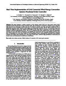
focus and thus the two systems are self-excited attractors. As investigated by many researchers [8–15], chaotic attractors with no equilibrium are hidden thus making NCS2 and NCS4 hidden attractors. 3.2. Lyapunov Exponents and Kaplan-Yorke Dimension. Lyapunov exponents of a nonlinear system define the convergence and divergence of the states. The existence of a positive Lyapunov exponent confirms the chaotic behavior of the system [38, 39]. Lyapunov exponents (LEs) are necessary and more convenient for detecting hyperchaos in fractional order hyperchaotic system. A definition of LEs for fractional differential systems was given in [40] based on frequencydomain approximations, but the limitations of frequencydomain approximations are highlighted by Tavazoei and Haeri [41]. Time series based LEs calculation methods like Wolf algorithm [11], Jacobian method [12], and neural network algorithm [13] are popularly known ways of calculating Lyapunov exponents for integer and fractional order systems. Hence we use the Jacobian method to calculate the LEs. Table 3 shows the Lyapunov exponents of the NCS. 3.3. Bifurcation. In this section we derive the bifurcation contours for the NCS. The chaotic behavior of the system largely depends on the parameters 𝑎, 𝑏, 𝑐, and 𝑑. As discussed in [42], the transient behaviors occurring in memristor based nonlinear systems may result in longer simulation times to reach steady states. Hence we used the ode45 solver for numerical simulations. Four different cases of bifurcations are investigated for the NCS. In case 1 the parameter 𝑎 is varied and the bifurcation of the attractor is investigated. Figure 5 shows the bifurcation plot for 𝑎. In the second case parameter 𝑏 is varied and the bifurcation of the NCS is studied which is shown in Figure 6. In case 3 the parameter 𝑐 is varied and bifurcation analysis of the system is investigated. Finally
bifurcation plot for parameter 𝑑 is derived in case 4. Figures 7 and 8 show the bifurcation contours of 𝑐 and 𝑑, respectively. As can be seen from the figures the NCS shows strange attractor, hyperchaos, chaos, and quasiperiodic systems. For 0 ≤ 𝑎 ≤ 0.25, 0.51 ≤ 𝑏 ≤ 0.72, 0.8 ≤ 𝑐 ≤ 1.2, and 1.34 ≤ 𝑑 ≤ 1.45 the NCS shows strange attractor and the transient behavior of the memristor prevents the bifurcation plots to show the period doubling property even after reducing the
transients to 70%. The system exhibits hyperchaotic attractor with hidden oscillations for 0.26 ≤ 𝑎 ≤ 0.8, 0.2 ≤ 𝑏 ≤ 0.5, 1.8 ≤ 𝑐 ≤ 2.3, and 1.04 ≤ 𝑑 ≤ 1.25. For a small band of 0 ≤ 𝑏 ≤ 0.1 with 0.8 ≤ 𝑎 ≤ 1.4, 2.4 ≤ 𝑐 ≤ 2.8, and 1.31 ≤ 𝑑 ≤ 1.45 the system shows chaotic oscillations with hidden attractors. A quasichaotic system is seen for 1.5 ≤ 𝑎 ≤ 1.8, 0.8 ≤ 𝑏 ≤ 2, 0.42 ≤ 𝑐 ≤ 0.7, and 1.47 ≤ 𝑑 ≤ 1.5. 3.4. Bicoherence. The motivation to study the bicoherence is twofold. First, the bicoherence can be used to extract information due to deviations from Gaussianity and suppress additive (colored) Gaussian noise. Second, the bicoherence can be used to detect and characterize asymmetric nonlinearity in signals via quadratic phase coupling or identify systems with quadratic nonlinearity. The bicoherence is the third-order spectrum. Whereas the power spectrum is a second-order statistic, formed from 𝑋 (𝑓) ∗ 𝑋(𝑓), where 𝑋(𝑓) is the Fourier transform of 𝑥(𝑡), the bispectrum is a third-order statistic formed from 𝑋(𝑓𝑗 ) ∗ 𝑋(𝑓𝑘 ) ∗ 𝑋 (𝑓𝑗 + 𝑓𝑘 ). The bispectrum is therefore a function of a pair of frequencies (𝑓𝑗 , 𝑓𝑘 ). It is also a complex-valued function. The (normalized) square amplitude is called the bicoherence (by analogy with the coherence from the cross-spectrum). The bispectrum is calculated by dividing the time series into 𝑀 segments of length 𝑁_seg, calculating their Fourier transforms and biperiodogram and then averaging over the ensemble. Although the bicoherence is a function of two frequencies the default output of this function is a onedimensional output, the bicoherence refined as a function of
60 40 20 0 W −20 −40 −60 26 24 22 20 18 16 14 12 10 Z
−4
−8
4
0
8
Y
Figure 4: 3D phase portraits of the NCS4 system.
60
10 8
40
6
20
4 Xmax
Xmax
2 0
0
−2
−20
−4
−40
−6 −60
−8 −10 0
0.5
1
1.5 a
2
2.5
−80
3
0
0.5
1
1.5
2
2.5
3
c
Figure 7: Bifurcation plots for parameter 𝑐.
Figure 5: Bifurcation plots for parameter 𝑎.
8
60
6
40
4
20
2 Xmax
Xmax
10 80
0 −20
0 −2
−40
−4
−60
−6
−80
−8
−100
−10 0
0.5
1
1.5
2
2.5 b
3
3.5
4
4.5
5
1.05
1.1
1.15
1.2
1.25 d
1.3
1.35
1.4
1.45
1.5
Figure 8: Bifurcation plots for parameter 𝑑.
Figure 6: Bifurcation plots for parameter 𝑏.
only the sum of the two frequencies. The autobispectrum of a chaotic system is given by Pezeshki et al. [43]. They derived the autobispectrum with the Fourier coefficients. 𝐵 (𝜔1 , 𝜔2 ) = 𝐸 [𝐴 (𝜔1 ) 𝐴 (𝜔2 ) 𝐴∗ (𝜔1 + 𝜔2 )] ,
1
(2)
where 𝜔𝑛 is the radian frequency and 𝐴 is the Fourier coefficients of the time series. The normalized magnitude spectrum
of the bispectrum known as the squared bicoherence is given by 𝑏 (𝜔1 , 𝜔2 ) =
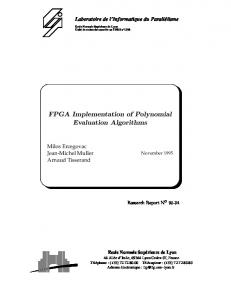
where 𝑃(𝜔1 ) and 𝑃(𝜔2 ) are the power spectrums at 𝑓1 and 𝑓2 . Figures 9 and 10 show the bicoherence contours of the NCS for 𝑎 ≠ 0 and 𝑏 ≠ 0 and 𝑎 = 0 and 𝑏 = 0,
Complexity
5 Power spectrum
0.3
reference frequency. Direct FFT is used to derive the power spectrum for individual frequencies and Hankel operator is used as the frequency mask. Hanning window is used as the FIR filter to separate the frequencies.
Power
0.2 0.1 0
0
0.05
0.1
0.15
0.2
0.25
0.3
0.35
0.4
0.45
0.5 0.
f/f fs
In this section we derive the fractional order model novel chaotic system (FONCS). There are three commonly used definitions of the fractional order differential operator, namely, those of Grunwald–Letnikov, Riemann–Liouville, and Caputo [23–25]. In this section, we will study the dynamical behavior of fractional order system derived from the NCS with the Grunwald-Letnikov (GL) definition, which is defined as
Theoretically fractional order differential equations use infinite memory. Hence when we want to numerically calculate or simulate the fractional order equations we have to use finite memory principal, where 𝐿 is the memory length and ℎ is the time sampling.
0.15 0.1 0.05 0
[(𝑡−𝑞)/ℎ]
where 𝑎 and 𝑡 are limits of the fractional order equation, 𝑞 Δ ℎ 𝑓(𝑡) is generalized difference, ℎ is the step size, and 𝑞 is the fractional order of the differential equation. For numerical calculations the above equation is modified as 𝑞 (𝑡−𝐿) 𝐷𝑡 𝑓 (𝑡)
respectively. As can be seen from the figures, the NCS shows wider band of power spectrum when 𝑎 ≠ 0 and 𝑏 ≠ 0 because of the hyperchaotic hidden attractor as when 𝑏 ≠ 0 the memristor element introduces a quadratic nonlinearity resulting in the cross-bicoherence. Shades in yellow represent the multifrequency components contributing to the power spectrum. From Figures 9 and 10 the cross-bicoherence is significantly nonzero and nonconstant, indicating a nonlinear relationship between the states. The yellow shades and nonsharpness of the peaks, as well as the presence of structure around the origin in figures (cross-bicoherence), indicate that the nonlinearity between the states 𝑥, 𝑦, 𝑧, and 𝑤 is not of the quadratic nonlinearity and hence may be because of nonlinearity of higher dimensions. The most two dominant frequencies (𝑓1 , 𝑓2 ) are taken for deriving the contour of bicoherence. The sampling frequency (𝑓𝑠 ) is taken as the
𝑡 𝐿 𝑁 (𝑡) = min {[ ] , [ ]} . ℎ ℎ
(6)
The binomial coefficients required for the numerical simulation are calculated as 𝑏𝑗 = (1 −
𝑎+𝑞 ) 𝑏𝑗−1 . 𝑗
(7)
Using (4)–(6) the fractional order NCS is defined as 𝐷𝑞𝑥 𝑥 = 15 (𝑦 − 𝑥) + 13𝑦𝑧, 𝐷𝑞𝑦 𝑦 = 18𝑥 − 𝑥𝑧 − 𝑏𝑥𝑊 (𝜙) − 𝑎, 𝐷𝑞𝑧 𝑧 = 𝑥𝑦 − 𝑐𝑧,
(8)
𝐷𝑞𝑤 𝑤 = −𝑑𝑥. As discussed in Section 1, the FONCS also shows chaotic and hyperchaotic systems with no equilibrium and single equilibrium points for a choice of parameter values 𝑎 and 𝑏 as shown in Table 4.
Figure 11: 3D phase portraits of NCS (𝑎 ≠ 0, 𝑏 ≠ 0).
28 26 24 22 20 Z 18 16 14 12 10 8 10
6
2
−2 Y
−6 −10 −100 −60
−20
20
60
X
−20 −30 −40 −50 W −60 −70 −80 −90 −100 −110 28
24
20
Z
16
12
8 −10
−6
2
−2
6
10
Y
Figure 12: 3D phase portraits of NCS (𝑎 ≠ 0, 𝑏 = 0).
Table 4: Choice of parameters and type of the system. Name of the system
Parameters 𝑎 and 𝑏
FONCS1
𝑎 = 0, 𝑏 = 0.5
FONCS2
𝑎 ≠ 0, 𝑏 = 0.5
FONCS3
𝑎 = 0, 𝑏 = 0
FONCS4
𝑎 ≠ 0, 𝑏 = 0
Type of system Hyperchaotic system with single equilibrium at origin Hyperchaotic system with no equilibrium Hyperchaotic system with single equilibrium at origin Chaotic system with no equilibrium
The 3D phase portraits of the FONCS are shown in Figures 11–14. The commensurate fractional orders of the system for 𝑎 = 0, 𝑏 ≠ 0, 𝑎 ≠ 0, 𝑏 ≠ 0, 𝑎 = 0, 𝑏 = 0, 𝑎 ≠ 0, and 𝑏 = 0 are taken as 𝑞 = 0.991, 𝑞 = 0.995, 𝑞 = 0.989, and 𝑞 = 0.990, respectively. 4.1. Dynamic Analysis of the FONCS. Most of the dynamic properties of the NCS like the Lyapunov exponents and bifurcation with parameters are preserved in the FONCS [44] if 𝑞𝑖 > 0.98, where 𝑖 = 𝑥, 𝑦, 𝑧, and 𝑤. The most important analysis of interest when investigating a fractional order system is the bifurcation with fractional order. The largest positive Lyapunov exponents (𝐿 1 = 19.8942, 𝐿 2 = 1.1436) of the NCS for 𝑎 = 0 and 𝑏 ≠ 0 appear when 𝑞 = 0.991 against their largest integer order Lyapunov exponents (𝐿 1 = 19.3050, 𝐿 2 = 1.0627), largest positive Lyapunov exponents
(𝐿 1 = 20.1613, 𝐿 2 = 1.4108) of the NCS for 𝑎 ≠ 0 and 𝑏 ≠ 0 appear when 𝑞 = 0.995 against their largest integer order Lyapunov exponents (𝐿 1 = 19.7244, 𝐿 2 = 1.2208), largest positive Lyapunov exponents (𝐿 1 = 3.8407, 𝐿 2 = 0.0134) of the NCS for 𝑎 = 0 and 𝑏 = 0 appear when 𝑞 = 0.989 against their largest integer order Lyapunov exponents (𝐿 1 = 3.51, 𝐿 2 = 0.0026) and largest positive Lyapunov exponent (𝐿 1 = 3.1187) of the NCS for 𝑎 ≠ 0 and 𝑏 = 0 appear when 𝑞 = 0.990 against its largest integer order Lyapunov exponent (𝐿 1 = 3.1029). It can also be seen that as the fractional order 𝑞 decreases, the FONCS starts losing its largest positive Lyapunov exponent. When 𝑞 ≤ 0.90 the positive Lyapunov exponents of the system become negative and thus the chaotic oscillation in the system disappears. Figures 15 and 16 show the bifurcation of the FONCS for variation in fractional orders 𝑞𝑥 = 𝑞𝑦 = 𝑞𝑧 = 𝑞𝑤 = 𝑞 for the two distinctive cases 𝑎 ≠ 0 and 𝑏 ≠ 0 and 𝑎 = 0 and 𝑏 = 0. 4.2. Stability Analysis of FONCS 4.2.1. Commensurate Order. For commensurate FONCS of order 𝑞, the system is stable and exhibits chaotic oscillations if |arg(eig(𝐽𝐸 ))| = |arg(𝜆 𝑖 )| > 𝑞𝜋/2, where 𝐽𝐸 is the Jacobian matrix at the equilibrium 𝐸 and 𝜆 𝑖 are the Eigenvalues of the FONCS, where 𝑖 = 1, 2, 3, and 4. As seen from the FONCS, the Eigenvalues should remain in the unstable region and the necessary condition for the FONCS to be stable is 𝑞 > (2/𝜋)tan−1 (|Im 𝜆|/Re 𝜆). The Eigenvalues of FONCS1 and FONCS3 are 𝜆 1 = 0; 𝜆 2 = −16.55; 𝜆 3 = 9.06; 𝜆 4 = −2 and 𝜆 3 is an unstable focus contributing to the existence of chaotic oscillations.
Complexity
28 26 24 22 Z 20 18 16 14 12 10 10
7
6
2
−2 Y
−6
−10 −80
−40
80
40
0
75 70 65 60 55 W 50 45 40 35 30 25
26
22
X
18 Z
14
10 −10 −6
−2
2
10
6
Y
Figure 13: 3D phase portraits of NCS (𝑎 = 0, 𝑏 = 0).
24 22 20 18 Z 16 14 12 10 8 8
4
0 Y
−4
−8
−80
−40
0 X
80
40
25 20 15 10 W 5 0 −5 −10 −15 24
20
16
Z
12
0 2 −4 −2 8 −8 −6 Y
4
6
8
24.5
80
24
70
23.5
60
23
50
22.5
40 Xmax
Xmax
Figure 14: 3D phase portraits of NCS (𝑎 = 0, 𝑏 ≠ 0).
Figure 15: Bifurcation of NCS versus fractional order 𝑞 (𝑎 ≠ 0, 𝑏 ≠ 0).
Figure 16: Bifurcation of NCS versus fractional order 𝑞 (𝑎 = 0, 𝑏 = 0).
4.2.2. Incommensurate Order. The necessary condition for the FONCS to exhibit chaotic oscillations in the incommensurate case is 𝜋/2𝑀 − min𝑖 (|arg(𝜆𝑖)|) > 0, where 𝑀 is the LCM of the fractional orders. If 𝑞𝑥 = 0.9, 𝑞𝑦 = 0.9, 𝑞𝑧 = 0.8, and 𝑞𝑤 = 0.8, then 𝑀 = 10. The characteristic equation of the system evaluated at the equilibrium is det(diag[𝜆𝑀𝑞𝑥 , 𝜆𝑀𝑞𝑦 , 𝜆𝑀𝑞𝑧 , 𝜆𝑀𝑞𝑤 ] − 𝐽𝐸) = 0 and by substituting the values of 𝑀 and the fractional orders, det(diag[𝜆9 , 𝜆9 , 𝜆8 , 𝜆8 ] − 𝐽𝐸 ) = 0, the characteristic equation is 𝜆34 + 2𝜆27 + 4𝜆26 + 15𝜆25 + 𝜆20 + 6𝜆19 + 35𝜆18 + 45𝜆17 − 300𝜆16 + 2𝜆12 + 21𝜆11 + 62𝜆10 − 570𝜆9 − 600𝜆8 + 𝜆4 + 17𝜆3 − 270𝜆2 − 600𝜆 and is the same for both FONCS1
and FONCS3 . The approximated solution of the characteristic equation is 𝜆 34 = 0.912 whose argument is zero and which is the minimum argument and hence the stability necessary condition becomes 𝜋/20 − 0 > 0 which solves for 0.0785 > 0 and hence the FONCS is stable and chaos exists in the incommensurate system.
5. FPGA Implementation of the Fractional Order Novel Cubic Nonlinear Systems In this section we discuss the implementation of the proposed FONCS in FPGA [21, 22, 38, 45–48] using the Xilinx (Vivado)
8
Complexity azerobnonzero_struct ce_1
x
clk_1 z
ce_1 clk_1
ce_1 clk_1
x_dot[31:0]
x1_out[31:0]
y[31:0]
z_dot[31:0]
z[31:0]
x[31:0]
azerobnonzero_x
y[31:0] azerobnonzero_z
x2_out[31:0] x3_out[31:0] y ce_1 clk_1 w[31:0]
y_dot[31:0]
x[31:0] z[31:0] azerobnonzero_y x4_out[31:0] w assert_m ce_1 clk_1
System Generator toolbox in Simulink. The challenge while implementing the systems in FPGAs is to design the fractional order integrator which is not a readily available block in the System Generator [21, 22]. Hence we implement the fractional integrators using the mathematical relation [32, 33] discussed in (4), (5), and (6) and the value of ℎ is taken as 0.001 with the initial conditions as described in Table 1
and the commensurate fractional order taken as 𝑞 = 0.991 for FONCS-1, 𝑞 = 0.995 for FONCS-2, 𝑞 = 0.989 for FONCS-3, and 𝑞 = 0.99 for FONCS-4. Figures 17, 18(a), and 18(b) show the Xilinx RTL schematics of the FONCS-1 system implemented in Kintex-7 (device = 7k160t, package = fbg484 S), power utilized by the system, and power utilized for various fractional orders, respectively. Table 5 shows the
Figure 19: 2D phase portraits of the FPGA implemented FONCS-1 system (𝑋𝑌, 𝑋𝑊, 𝑌𝑍, and 𝑍𝑊).
resources utilized by the FONCS-1 system including the clock frequency. Figure 19 shows the 2D state portraits of the FPGA implemented FONCS-1 system. Figures 20, 21(a), and 21(b) show the Xilinx schematics of the FONCS-2 system implemented in Kintex-7 (Device = 7k160t Package = fbg484 S), power utilized by the system and power utilization for various fractional orders, respectively. Table 6 shows the resources utilized by the FONCS-2 system including the clock frequency. Figure 22 shows the 2D state portraits of the FPGA implemented FONCS-2 system. Figures 23, 24(a), and 24(b) show the Xilinx schematics of the FONCS-3 system implemented in Kintex-7 (device = 7k160t, package = fbg484 S), power utilized by the system, and power utilization for
various fractional orders, respectively. Table 7 shows the resources utilized by the FONCS-3 system including the clock frequency. Figure 25 shows the 2D state portraits of the FPGA implemented FONCS-3 system. Figures 26, 27(a), and 27(b) show the Xilinx schematics of the FONCS-4 system implemented in Kintex-7 (device = 7k160t, package = fbg484 S), power utilized by the system, and power utilization for various fractional orders, respectively. Table 8 shows the resources utilized by the FONCS-3 system including the clock frequency. Figure 28 shows the 2D state portraits of the FPGA implemented FONCS-3 system. The sampling rates of the FPGA blocks play a crucial role in the existence of Lyapunov exponents and also increasing the sampling time
10
Complexity abnotzero_struct
ce_1
x
clk_1 z
ce_1 clk_1
ce_1 clk_1
x1_dot[31:0]
x1_out[31:0]
y[31:0]
x3_dot[31:0]
z[31:0]
x[31:0]
abnotzero_x
y[31:0] abnotzero_z
x2_out[31:0] x3_out[31:0] y ce_1 clk_1 w[31:0]
x2_dot[31:0]
x[31:0] z[31:0] abnotzero_y x4_out[31:0] w assert_m ce_1 clk_1
Figure 21: (a) Power utilized and (b) power utilization versus fractional order of FONCS-2 system.
1
Complexity
Y
11
6
22
4
20
2
18
0 −2
W 16 14
−4
12
−6
10
−60
−40
−20
0 X
20
40
22 20 18 Z
16 14 12 10 8
−6
−4
−2
0
2
4
8 −60
60
6
30 25 20 15 W 10 5 0 −5 −10
8
−40
10
−20
12
0 X
20
14
16
40
18
20
60
22
Z
Y
Figure 22: 2D phase portraits of the FPGA implemented FONCS-2 system (𝑋𝑌, 𝑋𝑊, 𝑌𝑍, and 𝑍𝑊). abzero_struct
x ce_1 x_dot[31:0]
clk_1 y[31:0]
z
w
z[31:0] ce_1
ce_1
clk_1
clk_1
ce_1
abzero_x
w_dot[31:0]
clk_1
x[31:0]
z_dot[31:0]
x[31:0]
y
y[31:0]
abzero_w
z[31:0]
x1_out[31:0]
ce_1 y_dot[31:0]
clk_1
abzero_z
x2_out[31:0] x3_out[31:0]
x[31:0]
x4_out[31:0]
z[31:0] abzero_y
assert_m din[31:0]
dout[31:0]
xlpassthrough abzero_struct
Figure 23: RTL schematics of FONCS-3 system.
period in some implementations may lead to a clock frequency mismatch. Maximum power will be consumed by the system when the FONCS shows largest Lyapunov exponents (FONCS-1 𝑞 = 0.991, FONCS-2 𝑞 = 0.995, and FONCS-3 𝑞 = 0.996). To utilize the power of FPGA, the computation needs to be divided into several independent blocks of threads that can be executed simultaneously [39, 49]. The FONCS power efficiency also depends on the parameter 𝑏 as can be observed from the power efficiency Figures 18, 21, 24, and 27. When 𝑏 ≠ 0 the FONCS uses a maximum power of 299 w against
280 w when 𝑏 = 0. This is because of the reason that the system shows their largest positive Lyapunov exponents when 𝑏 ≠ 0. The effect of parameter 𝑎 on the power efficiency is quiet minimal and negligible. The performance on FPGA is directly related to the number of threads and its performances and hence the FONCS are designed as four parallel threads. The fractional order operators are implemented as building blocks and the so-called “frame delay” is not noticeable in the FPGA hardware implementation due to its parallel data structure, unlike a microprocessor-based implementation.
Figure 28: 2D phase portraits of the FPGA implemented FONCS-4 system.
Table 8: Resource utilization of FONCS-4 system. Resource
Utilization
Available
Utilization %
911 256 12 129 1
101400 202800 600 285 32
0.90 0.13 2.00 45.26 3.13
LUT FF DSP IO BUFG
6. Conclusion This paper introduces a new hyperchaotic system which when changing the values of parameters exhibits self-excited and hidden attractors. Dynamic analyses of the proposed hyperchaotic system are investigated. Fractional order model of the hyperchaotic system is derived and implemented in FPGA. Power efficiency analyses for various fractional orders are derived and it is shown that the system uses maximum power when exhibiting its largest Lyapunov exponent.
Conflicts of Interest The authors declare that there are no conflicts of interest regarding the publication of this paper.
Acknowledgments The authors wish to extend their sincere thanks and gratitude to Dr. Sajad Jafari, Department of Biomedical Engineering,
Amirkabir University of Technology, for guiding in achieving crucial results.
References [1] G. A. Leonov, N. V. Kuznetsov, and V. I. Vagaitsev, “Localization of hidden Chua’s attractors,” Physics Letters A, vol. 375, no. 23, pp. 2230–2233, 2011. [2] G. A. Leonov, N. V. Kuznetsov, and V. I. Vagaitsev, “Hidden attractor in smooth Chua systems,” Physica D. Nonlinear Phenomena, vol. 241, no. 18, pp. 1482–1486, 2012. [3] G. A. Leonov and N. V. Kuznetsov, “Hidden attractors in dynamical systems. From hidden oscillations in HilbertKolmogorov, Aizerman, and Kalman problems to hidden chaotic attractor in Chua circuits,” International Journal of Bifurcation and Chaos, vol. 23, no. 01, Article ID 1330002, 2013. [4] G. A. Leonov, N. V. Kuznetsov, and T. N. Mokaev, “Hidden attractor and homoclinic orbit in Lorenz-like system describing convective fluid motion in rotating cavity,” Communications in Nonlinear Science and Numerical Simulation, vol. 28, no. 1–3, pp. 166–174, 2015.
Complexity [5] G. A. Leonov, N. V. Kuznetsov, and T. N. Mokaev, “Homoclinic orbits, and self-excited and hidden attractors in a Lorenzlike system describing convective fluid motion,” The European Physical Journal Special Topics, vol. 224, no. 8, pp. 1421–1458, 2015. [6] P. R. Sharma, M. D. Shrimali, A. Prasad, N. V. Kuznetsov, and G. A. Leonov, “Control of multistability in hidden attractors,” The European Physical Journal: Special Topics, vol. 224, no. 8, pp. 1485–1491, 2015. [7] P. R. Sharma, M. D. Shrimali, A. Prasad, N. V. Kuznetsov, and G. A. Leonov, “Controlling dynamics of hidden attractors,” International Journal of Bifurcation and Chaos, vol. 25, no. 4, Article ID 1550061, 2015. [8] S. Jafari, J. C. Sprott, V.-T. Pham, S. M. Hashemi Golpayegani, and A. Homayoun Jafari, “A new cost function for parameter estimation of chaotic systems using return maps as fingerprints,” International Journal of Bifurcation and Chaos, vol. 24, no. 10, Article ID 1450134, 2014. [9] V.-T. Pham, C. Volos, S. Jafari, Z. Wei, and X. Wang, “Constructing a novel no-equilibrium chaotic system,” International Journal of Bifurcation and Chaos in Applied Sciences and Engineering, vol. 24, no. 5, Article ID 1450073, 6 pages, 2014. [10] F. R. Tahir, S. Jafari, V.-T. Pham, C. Volos, and X. Wang, “A novel no-equilibrium chaotic system with multiwing butterfly attractors,” International Journal of Bifurcation and Chaos in Applied Sciences and Engineering, vol. 25, no. 4, 2015. [11] S. Jafari, V.-T. Pham, and T. Kapitaniak, “Multiscroll chaotic sea obtained from a simple 3D system without equilibrium,” International Journal of Bifurcation and Chaos, vol. 26, no. 2, Article ID 1650031, 2016. [12] S.-K. Lao, Y. Shekofteh, S. Jafari, and J. C. Sprott, “Cost function based on Gaussian mixture model for parameter estimation of a chaotic circuit with a hidden attractor,” International Journal of Bifurcation and Chaos in Applied Sciences and Engineering, vol. 24, no. 1, 2014. [13] S. Jafari, V.-T. Pham, and T. Kapitaniak, “Multiscroll chaotic sea obtained from a simple 3D system without equilibrium,” International Journal of Bifurcation and Chaos, vol. 26, no. 2, Article ID 1650031, 2016. [14] V.-T. Pham, S. Vaidyanathan, C. Volos, S. Jafari, and S. T. Kingni, “A no-equilibrium hyperchaotic system with a cubic nonlinear term,” Optik, vol. 127, no. 6, pp. 3259–3265, 2016. [15] V.-T. Pham, S. Vaidyanathan, C. K. Volos, S. Jafari, N. V. Kuznetsov, and T. M. Hoang, “A novel memristive time–delay chaotic system without equilibrium points,” European Physical Journal: Special Topics, vol. 225, no. 1, pp. 127–136, 2016. [16] M. Molaie, S. Jafari, J. C. Sprott, and S. M. R. H. Golpayegani, “Simple chaotic flows with one stable equilibrium,” International Journal of Bifurcation and Chaos, vol. 23, no. 11, Article ID 1350188, 2013. [17] S. T. Kingni, S. Jafari, H. Simo, and P. Woafo, “Threedimensional chaotic autonomous system with only one stable equilibrium: analysis, circuit design, parameter estimation, control, synchronization and its fractional-order form,” The European Physical Journal Plus, vol. 129, no. 5, pp. 1–16, 2014. [18] M. Molaie, S. Jafari, J. C. Sprott, and S. M. Hashemi Golpayegani, “Simple chaotic flows with one stable equilibrium,” International Journal of Bifurcation and Chaos in Applied Sciences and Engineering, vol. 23, no. 11, Article ID 1350188, 7 pages, 2013. [19] S. T. Kingni, S. Jafari, H. Simo, and P. Woafo, “Threedimensional chaotic autonomous system with only one stable
15 equilibrium: analysis, circuit design, parameter estimation, control, synchronization and its fractional-order form,” The European Physical Journal Plus, vol. 129, no. 5, article 76, pp. 1– 16, 2014. [20] V. Pham, S. Jafari, C. Volos, A. Giakoumis, S. Vaidyanathan, and T. Kapitaniak, “A chaotic system with equilibria located on the rounded square loop and its circuit implementation,” IEEE Transactions on Circuits and Systems II: Express Briefs, vol. 63, no. 9, pp. 878–882, 2016. [21] R. Karthikeyan, A. Prasina, R. Babu, and S. Raghavendran, “FPGA implementation of novel synchronization methodology for a new chaotic system,” Indian Journal of Science and Technology, vol. 8, no. 11, 2015. [22] K. Rajagopal, A. Karthikeyan, and A. K. Srinivasan, “FPGA implementation of novel fractional-order chaotic systems with two equilibriums and no equilibrium and its adaptive sliding mode synchronization,” Nonlinear Dynamics. An International Journal of Nonlinear Dynamics and Chaos in Engineering Systems, vol. 87, no. 4, pp. 2281–2304, 2017. [23] D. Baleanu, K. Diethelm, E. Scalas, and J. J. Trujillo, Fractional Calculus: Models and Numerical Methods, World Scientific, Singapore, 2014. [24] Y. Zhou, Basic Theory of Fractional Differential Equations, World Scientific, Singapore, 2014. [25] K. Diethelm, The Analysis of Fractional Differential Equations, Springer, Berlin, Germany, 2010. [26] M. Pourmahmood Aghababa, “Robust finite-time stabilization of fractional-order chaotic systems based on fractional lyapunov stability theory,” Journal of Computational and Nonlinear Dynamics, vol. 7, no. 2, Article ID 021010, 2012. [27] E. A. Boroujeni and H. R. Momeni, “Non-fragile nonlinear fractional order observer design for a class of nonlinear fractional order systems,” Signal Processing, vol. 92, no. 10, pp. 2365–2370, 2012. [28] R. Zhang and J. Gong, “Synchronization of the fractional-order chaotic system via adaptive observer,” Systems Science & Control Engineering, vol. 2, no. 1, pp. 751–754, 2014. [29] R. H. Li and W. S. Chen, “Complex dynamical behavior and chaos control in fractional-order Lorenz-like systems,” Chinese Physics B, vol. 22, no. 4, Article ID 040503, 2013. [30] D. Cafagna and G. Grassi, “Fractional-order systems without equilibria: the first example of hyperchaos and its application to synchronization,” Chinese Physics B, vol. 24, no. 8, Article ID 080502, 2015. [31] M.-F. Danca, W. K. Tang, and G. Chen, “Suppressing chaos in a simplest autonomous memristor-based circuit of fractional order by periodic impulses,” Chaos, Solitons & Fractals, vol. 84, pp. 31–40, 2016. [32] I. Petras, “Methos for simulation of the fractional order chaotic systems,” Acta Montanastica Slovaca, vol. 11, no. 4, pp. 273–277, 2006. [33] W. Trzaska Zdzislaw, Matlab Solutions of Chaotic Fractional Order Circuits, InTech, Rijeka, Croatia, 2013, http://www.intechopen.com/download/pdf/21404. [34] M. A. Jafari, E. Mliki, A. Akgul et al., “Chameleon: the most hidden chaotic flow,” Nonlinear Dynamics, pp. 1–15, 2017. [35] Q. Li, H. Zeng, and J. Li, “Hyperchaos in a 4D memristive circuit with infinitely many stable equilibria,” Nonlinear Dynamics, vol. 79, no. 4, pp. 2295–2308, 2015.
16 [36] Q.-H. Hong, Y.-C. Zeng, and Z.-J. Li, “Design and simulation of chaotic circuit for flux-controlled memristor and chargecontrolled memristor,” Acta Physica Sinica, vol. 62, no. 23, Article ID 230502, 2013. [37] S. Sampath, S. Vaidyanathan, and V.-T. Pham, “A novel 4-D hyperchaotic system with three quadratic nonlinearities, its adaptive control and circuit simulation,” International Journal of Control Theory and Applications, vol. 9, no. 1, pp. 339–356, 2016. [38] V. Rashtchi and M. Nourazar, “FPGA implementation of a realtime weak signal detector using a duffing oscillator,” Circuits, Systems, and Signal Processing, vol. 34, no. 10, pp. 3101–3119, 2015. [39] E. Tlelo-Cuautle, J. J. Rangel-Magdaleno, A. D. Pano-Azucena, P. J. Obeso-Rodelo, and J. C. Nunez-Perez, “FPGA realization of multi-scroll chaotic oscillators,” Communications in Nonlinear Science and Numerical Simulation, vol. 27, no. 1–3, pp. 66–80, 2015. [40] C. Li, Z. Gong, D. Qian, and Y. Chen, “On the bound of the Lyapunov exponents for the fractional differential systems,” Chaos, vol. 20, no. 1, Article ID 013127, 2010. [41] M. S. Tavazoei and M. Haeri, “Unreliability of frequencydomain approximation in recognising chaos in fractional-order systems,” IET Signal Processing, vol. 1, no. 4, pp. 171–181, 2007. [42] B. Bao, P. Jiang, H. Wu, and F. Hu, “Complex transient dynamics in periodically forced memristive Chua’s circuit,” Nonlinear Dynamics, vol. 79, no. 4, pp. 2333–2343, 2015. [43] C. Pezeshki, S. Elgar, and R. C. Krishna, “Bispectral analysis of systems possessing chaotic motion,” Journal of Sound and Vibration, vol. 137, no. 3, pp. 357–368, 1990. [44] D. Dudkowski, S. Jafari, T. Kapitaniak, N. V. Kuznetsov, G. A. Leonov, and A. Prasad, “Hidden attractors in dynamical systems,” Physics Reports. A Review Section of Physics Letters, vol. 637, pp. 1–50, 2016. [45] E. Tlelo-Cuautle, A. D. Pano-Azucena, J. J. Rangel-Magdaleno, V. H. Carbajal-Gomez, and G. Rodriguez-Gomez, “Generating a 50-scroll chaotic attractor at 66 MHz by using FPGAs,” Nonlinear Dynamics, vol. 85, no. 4, pp. 2143–2157, 2016. [46] Q. Wang, S. Yu, C. Li et al., “Theoretical design and FPGA-based implementation of higher-dimensional digital chaotic systems,” IEEE Transactions on Circuits and Systems I-Regular Papers, vol. 63, no. 3, pp. 401–412, 2016. [47] E. Dong, Z. Liang, S. Du, and Z. Chen, “Topological horseshoe analysis on a four-wing chaotic attractor and its FPGA implement,” Nonlinear Dynamics, vol. 83, no. 1-2, pp. 623–630, 2016. [48] E. Tlelo-Cuautle, V. H. Carbajal-Gomez, P. J. Obeso-Rodelo, J. J. Rangel-Magdaleno, and J. C. N´un˜ ez-P´erez, “FPGA realization of a chaotic communication system applied to image processing,” Nonlinear Dynamics, vol. 82, no. 4, pp. 1879–1892, 2015. [49] Y.-M. Xu, L.-D. Wang, and S.-K. Duan, “A memristor-based chaotic system and its field programmable gate array implementation,” Wuli Xuebao/Acta Physica Sinica, vol. 65, no. 12, Article ID 120503, 2016.
Complexity
Advances in
Operations Research Hindawi Publishing Corporation http://www.hindawi.com