Sep 19, 2002 - Data layout in memory of key variables is important for applications programs that make use ... â E-mail: {k.a.hawick, d.p.playne}@massey.ac.nz.
CONCURRENCY AND COMPUTATION: PRACTICE AND EXPERIENCE Concurrency Computat.: Pract. Exper. 2010; 00:1–27 Prepared using cpeauth.cls [Version: 2002/09/19 v2.02]
Hypercubic Storage Layout and Transforms in Arbitrary Dimensions using GPUs and CUDA K.A. Hawick∗ and D.P. Playne† Institute of Information and Mathematical Sciences, Massey University – Albany, North Shore 102-904, Auckland, New Zealand.
SUMMARY Many simulations in the physical sciences are expressed in terms of rectilinear arrays of variables. It is attractive to develop such simulations for use in 1-, 2-, 3- or arbitrary physical dimensions and also in a manner that supports exploitation of data-parallelism on fast modern processing devices. We report on data layouts and transformation algorithms that support both conventional and data-parallel memory layouts. We present our implementations expressed in both conventional serial C code as well as in NVIDIA’s Compute Unified Device Architecture (CUDA) concurrent programming language for use on General Purpose Graphical Processing Units (GPGPU). We discuss: general memory layouts; specific optimisations possible for dimensions that are powers-of-two; and common transformations such as inverting, shifting and crinkling. We present performance data for some illustrative scientific applications of these layouts and transforms using several current GPU devices and discuss the code and speed scalability of this approach. KEY WORDS :
1.
data-parallelism; GPUs; CUDA; shifting; crinkling; hypercubic indexing.
INTRODUCTION
Data layout in memory of key variables is important for applications programs that make use of dataparallelism. Several well-known applications such as image processing and lattice models make use of rectilinear data that can be mapped closely to the parallel processing structure of a data-parallel computer. Many other applications and particularly numerical simulations in physics, chemistry and other areas of science and engineering are oriented around hypercubic data arrays where there is a high degree of potential parallelism to be exploited in the calculations. It is not always the case however that the logical data layout for the serial application program or from some file storage format is the
∗ Correspondence † E-mail:
to: IIMS Massey University – Albany, North Shore 102-904, Auckland, NZ. {k.a.hawick, d.p.playne}@massey.ac.nz
c 2010 John Wiley & Sons, Ltd. Copyright
Received 23 June 2009 Revised 12 April 2010
2
K. A. HAWICK AND D. P. PLAYNE
optimal data-parallel layout for the target compute platform. Often a stencil-oriented algorithm, such as for image processing [1] or lattice-based Monte Carlo simulations [2,3], requires neighbouring adjacent data to remain unchanged during a synchronous update operation. Consequently some data-striding or array-crinkling is necessary to apply data-parallel concurrent updates. Fine-grained data-parallelism is going through a revival period largely due to the low cost, wide availability and relative ease of programmability of processing accelerator devices such as Graphical Processing Units (GPUs) [4]. These devices can be programmed using a data-parallel approach using relatively high level languages such as NVIDIA’s Compute Unified Device Architecture (CUDA) language. The term general-purpose GPU programming (GPGPU) [5] is now widely used to describe this rapidly growing applications-level use of GPU hardware [6, 7, 8]. Many of the ideas of data-parallelism were first invented and explored for the massively parallel, single-instruction multiple-data (SIMD) computers of the period between the mid 1970s and early 1990s. Computers such as the Distributed Array Processor (DAP) [9, 10], the Connection Machine (CM) [11] and MasPar [12] had software libraries [13, 14] with built-in routines for data layout transformations on regular rectilinear data structures. These machines often achieved notably high performance [15] on appropriately sized and shaped data structures [16] in scientific simulations [17] and related applications. The power of these machines also inspired the development of many dataparallel software libraries, kernels [18, 19] and programming languages [20, 21, 22, 23] that are still in use. We refer to the notion of data crinkling - a concept that appears to have its origins with array processing. The term comes from the notion of folding or crinkling a sheet of paper so that some elements are subsequently much closer together than before. Crinkling is an operation and as such described more than just data striding through memory. The DAP supported two dimensional crinkling [24] whereupon “normal” or serially laid-out data from the host computer’s memory could be crinkled or uncrinkled to block it in different ways depending on what was optimal for the application’s algorithms that ran on the array-processor accelerator [25]. Graphical Processing Units (GPUs) have much in common with computers such as the DAP, CM and MasPar. GPUs are programmed as special subroutines (known as kernels in CUDA) that are called from the conventional serial program running on the host processor. Thus an application consists of a CPU program linked to one or more GPU program components and will make use of various special purpose data allocation and transfer routines between CPU and GPU memory. Although there have been several programmer systems and tools for exploiting GPUs [26, 27, 28, 29], NVIDIA’s CUDA language has emerged as one of the most powerful for scientific applications [30]. While CUDA is presently specific to NVIDIA hardware, the Open Compute Language (OpenCL) promises similar capabilities and applications programmer accessibility. Nevertheless, exploiting parallel computing effectively at an applications level remains a challenge for programmer. In this article we focus on data layout and storage transforms and explore the detailed coding techniques and performance optimisation techniques offered by CUDA [8] to build software for shifting, crinkling and re-indexing hypercubic data in arbitrary dimensions. Managing optimal data layout on parallel computing systems is not a trivial problem [31] and in a complex application there may not be one single data layout that is optimal for all sub-algorithmic components of the code [32]. It is therefore valuable for a data-parallel system to have an appropriate library of data-transformation routines such as the parallel data transforms (PDTs) of Flanders and Reddaway [33]. A number of attempts have been made to optimise the PDT ideas using bit-wise operations that were customised for particular data sizes (such as powers-of-two) [34,35] that naturally
c 2010 John Wiley & Sons, Ltd. Copyright Prepared using cpeauth.cls
Concurrency Computat.: Pract. Exper. 2010; 00:1–27
HYPERCUBIC INDEXING WITH CUDA
3
fit onto particular hardware. Other work has also considered using indexing reshuffles to minimise memory usage by avoiding vacant elements in sparse or compressible structures [36]. Attempts have also been made to generalise the data transform ideas algebraically [37,38,39]. Most research went into optimising the ideas for two dimensional image data [40,41] on computers such as the MasPar [42,43] or DAP [44]. In this article we consider how the parallel data-transform ideas can be implemented using CUDA-like programming languages for performance, but also more generally in plain ordinary serial languages like C for portability reasons and for interoperability between CPU-Host/GPU-Accelerator program combinations. The multiple threads and grid-block model used for GPUs requires some important new approaches that depart from the indexing model that was optimal for computers like the DAP, CM and MasPar. The GPU memory model is in fact quite complex and comes in several different sorts with different layout and speed characteristics. We consider data that is logically treated as a hypercubic array of arbitrary dimensions, but which can be mapped to contiguous main memory for the CPU to access, yet suitably transformed to an optimal layout for an associated GPU to work with. We have investigated both dimensions that are powers-of-two and multiples of the GPU specialist memory length and size parameters, but also general unconstrained values. In Section 2 we give a brief review of the GPU memory architecture. We outline the main data notation and hypercubic data layout ideas in Section 3 followed by a description of a generalised data indexing system in Section 4. We describe how the indexing can be optimised using bit-wise operations in Section 5 and discuss the issues and approaches to optimal data neighbour access and indexing in Section 6. In Section 7 we describe our CUDA implementation of the hypercubic indexing and also present code and algorithms for shifting and crinkling transforms in Section 8. We present some performance results using NVIDIA GeForce 9400/9600, 260 and 295 GPUs in Section 10. In Section 11 we discuss the implications for applications that use hypercubic storage transforms and offer some conclusions and areas for future optimisation work.
2.
GPU ARCHITECTURE SUMMARY
Modern GPUs contain many processor cores that can execute instructions in parallel. A typical GPU (such as one of the NVIDIA GeForce 200 series) contains 16-60 multi-processors, each of which contains 8 scalar processor cores (giving a processor total of 128-480). These GPUs are capable of managing, scheduling and executing many threads at once using the SIMT paradigm [45]. To make use of the parallel computational power of a GPU, an application must be decomposed into many parallel threads. One difference between decomposing an application onto a common distributed or parallel architecture and a GPU is the number of threads required. GPUs provide the best performance when executing 1000+ threads. These threads are organised as a grid of thread blocks. Each thread block contains a maximum of 512 threads and the grid size is limited to {65535, 65535, 1}. Each thread has a threadIdx which determines its id within a block and a blockIdx which determines the id of the block it belongs to. From these two identifiers, each thread can calculate its unique id. GPUs also contain many memory types optimised for different tasks. These optimisations were developed for increased performance when processing the graphics pipeline but they can be easily
c 2010 John Wiley & Sons, Ltd. Copyright Prepared using cpeauth.cls
Concurrency Computat.: Pract. Exper. 2010; 00:1–27
4
K. A. HAWICK AND D. P. PLAYNE
utilised for other purposes. Selecting the memory type best suited to the access pattern is vital to the performance of a GPU application [46], but equally as important is the memory access pattern used. Global memory is the largest type of memory available on the GPU and can be accessed by all threads, unfortunately it is also the slowest. Access to global memory can be improved by a method known as coalescing [45]. If 16 sequential threads access 16 sequential (and aligned) memory addresses in global memory, the accesses can be combined into a single transaction. This can greatly improve performance of a GPU program that uses global memory. Texture and Constant memory are both cached methods for accessing global memory. Texture memory caches the values in a spatial locality (near neighbours in the dimensionality of the texture) allowing neighbouring threads to access neighbouring values from global memory whereas constant memory allows multiple threads to access the same value from memory simultaneously. Each multiprocessor has its own texture and constant memory cache. Shared memory is also stored on the multiprocessor but must be explicitly written to and read from by the threads in the multiprocessor. This memory is useful for threads that must share data or perform some primitive communication. Registers and Local memory are used for the local variables used within the threads. The registers are stored on the multi-processor itself whereas local memory is actually just global memory but used for local variables. The threads will use the registers first and if necessary will make use of local memory, it is preferable if only the registers are used.
3.
DATA LAYOUT ISSUES AND NOTATION
In this section we discuss the fundamental ideas behind expressing dimensions, shapes and layouts for hypercubic or rectilinear data arrays. We are considering a d-dimensional space Rd , spanned by r = (r0 , ..., rd−1 ). In most cases we are interested in a physical space and d = 2, 3; however, in some cases we wish to simulate systems with d = 4, 5 and higher. Certainly the mapping problem of real space to data structure generally simplifies considerably when d ≡ 1 where we simply have an ordered list. A simple integer index i maps to the spatial region or 1-dimensional interval associated with r and in many cases the mapping is a simple one, with the interval spacing ∆ being constant [47]. Thus we have: ri = r0 + i × ∆, ∀i = 0, 1, ..., L − 1 (1) with the r0 value chosen to determine the origin. However, when programming multi-dimensional spaces we typically want to use index i over the dimensions. When working with real space with 2 or more dimensions, we define d-dimensions as: rx0 , ...rxd−1 . To work with these, we must employ some sort of spatial mapping between a discrete index-tuple xi and the spatial cell or region associated with it. rx0 rx1
= =
r00 + x0 × ∆0 , ∀x0 r10 + x1 × ∆1 , ∀x1
rxd−1
··· =
0 rd−1 + xd−1 × ∆d−1 , ∀xd−1 = 0, 1, ..., Ld−1 − 1
c 2010 John Wiley & Sons, Ltd. Copyright Prepared using cpeauth.cls
= 0, 1, ..., L0 − 1 = 0, 1, ..., L1 − 1 (2)
Concurrency Computat.: Pract. Exper. 2010; 00:1–27
5
HYPERCUBIC INDEXING WITH CUDA
Often for a simple program the ∆d values in each dimension are all the same value, perhaps even unity if the spatial units of the system modelled can be so adjusted. In all our examples we have made use of indexing from 0, ..., L − 1 as it is the generally accepted index methods by most modern programming languages. Within a programming environment we can often define this d-dimensional space as a d-dimensional array. When defining a multi-dimensional array is it important to consider each programming language’s built in multi-dimensional array indexing approach to allow for the best memory paging access. In Fortran we could implement REAL SPACE(0:L1-1, 0:L2-1, 0:L3-1) where the data is laid out in memory column major so the first index is fastest changing whereas in C/C++ we would declare: double space[L3][L2][L1] where we have had to reverse the order of dimensions so that index 0 is fastest changing in memory, based on the row-major ordering used by C. One disadvantage of representing a multi-dimensional space as a multi-dimensional array is the significant restructuring process required when the number of dimensions is changed. Instead there is a more general method of representing multi-dimensional space. We want an unambiguous notation to specify these transformations and also an efficient set of algorithms to perform these operations, either in place or as a fresh data-set copy. Ideally the notation should map well to the array or operational syntax of a programming language. We also want to be able to perform combination operations on the transformations to make composites that can be executed in a single operation, again preferably in parallel. [L2 , L1 , L0 ]
(3)
implies data that is 3-dimensional (d ≡ 3) with lengths Li in each dimension. We sometimes need to explicitly consider the type of the data. This specifies the size or storage requirement of each individual data element. We might think about it as unambiguous bits, and so write it as [128, 128, 128, 32] (4) for an array of 32-bit ints for example. We could also write the type using some mnemonic such as: [128, 128, 128, int32]
(5)
[128, 128, 128, 4, 8]
(6)
and we could treat this as where we have 4 bytes per int and of course 8 bits per byte. Although this notation might seem verbose or clumsy, it is useful because it is completely unambiguous - a bit is a bit is a bit and cannot be mistaken for something else, whereas a word or even the byte order in a word can differ between machine implementations. This ambiguity has been a barrier to portable use of some of the data-transform algorithms and implementations supplied by SIMD computer vendors in the past. The notation implies a minimal sequential storage size d−1 Li N = Πi=0
(7)
and we can think of the data as indexed in a fundamental way using a k-index where k = 0, 1, ..., N −1 with the usual convention for least significant dimension to the right, most significant dimension to the left.
c 2010 John Wiley & Sons, Ltd. Copyright Prepared using cpeauth.cls
Concurrency Computat.: Pract. Exper. 2010; 00:1–27
6
K. A. HAWICK AND D. P. PLAYNE
This k-index idea is similar to the single array reference idea mentioned in [48] where Ciernak and Li use it to restructure linear algebra operations instead of using two array indices to access matrices. The idea can be generalised however so that we can write arbitrary dimensional simulations using a single k-index and therefore do not need to know how many explicit nested loops to write in the program. We can also ascribe spatial encoding information to the k-index as we discuss below in section 4. We can combine these specifiers by multiplication and we get the same implied resulting dimension and storage size regardless of associative order. The interpretation is different however. It is useful for example to drop the data type part and decompose: [128, 128, 128, 32] 7→ [128, 128, 128] · [32]
(8)
or D2 · D1 . We can then do operations or algebra on D2 , while temporarily ignoring the notion that each individual element is of type D1 . We want to be able to apply transformations or remappings to the data to be able to interpret it in different ways. So data set D2 that is in layout L1 can be transformed into a different layout L2 with the same fundamental size or it can be filtered or reduced to a smaller data set. We might also allow duplications or insertions of padded zeros into the source for example and thus arrive at a larger target data set. These general ideas lead onto a specific approach using a single compressed index into sequential contiguous storage space. This approach is well known and widely used in various applications, but does not seem to have a widely used name. We refer to it as k-indexing using a single integer k that compresses all information about all the data dimensions. It is particularly useful for writing simulation codes in arbitrary dimension without embedding a fixed number of nested for-loops in the source code.
4.
HYPERCUBIC k-INDEXING
The technique we call k-indexing makes use of integer calculations within the user’s application programming to index into a single-dimensional array or block of memory. In the case of a dense and regular space we can readily map between our model indices xi , i = 0, 1, ..., d − 1 and a memory index k which is solely a memory addressing index. It is convenient to adopt notation so that each dimension is labelled by i = 0, 1, ..., d − 1 and the lengths of the regular space, in units of the appropriate ∆i , for each dimension are Li such that xi is in the range [0...Li − 1]. Thus we can calculate the k-index completely generally from: k = x0 + L0 × x1 + L0 × L1 × x2 + L0 × L1 × L2 × x3 + · · ·
(9)
We can decompose a k-index into individual dimensional indexes by an orthogonalisation process, assuming we have available a modulo operation (denoted throughout this article by %.) xi =
k %Li L0 × L1 · · · Li−1
(10)
This is more complicated than it looks but can be implemented as an iteration over the dimensions:
c 2010 John Wiley & Sons, Ltd. Copyright Prepared using cpeauth.cls
Concurrency Computat.: Pract. Exper. 2010; 00:1–27
HYPERCUBIC INDEXING WITH CUDA
7
Listing 1. Construction of a k-index from individual indexes and decomposition into indexes. / / c o n s t r u c t a k−i n d e x f r o m an i n d e x −v e c t o r i n t toK ( i n t ∗x ) { i n t k = 0 , LP = 1 ; f o r ( i n t i = 0 ; i < d ; i ++ ) { k += x [ i ] ∗ LP ; LP ∗= L [ i ] ; } return k ; } / / decompose a k−i n d e x i n t o an i n d e x −v e c t o r v o i d fromK ( i n t ∗x , i n t k ) { i n t LP = N ; f o r ( i n t i = d −1; i >= 0 ; i −−) { LP / = L [ i ] ; x [ i ] = k / LP ; k = k % LP ; } }
Alternatively we could pre-compute the Ld products as used in Equation 10 and these could available in a globallyQ accessible array LP[], bound to the hypercubic data set in question. We implement this i as LP[i] = j=0 Lj so that LP[i] is the stride (for normal data layout on the serial host memory) in dataset dimension i. For example, a data set of size N = 64 = 4 × 4 × 4 elements would have LP ≡ {1, 4, 16, 64}. Also note our convention that our index-vector is indexed both in the programming language and the formulae given Q here using dimension i = 0, 1, ..., d − 1. The k-index formed runs from 0, ..., N − 1 where N = i Li is the total number of spatial cells in our dense representation of space. Figure 1 shows an indirect addressing scheme that is useful for hyper-cubic symmetry lattice models in arbitrary dimension d. The lattice lengths Li , i = 0, ..., d − 1 in each dimension are fixed and hence cell positions xi , i = 0, ..., d − 1 on the lattice can be encoded as a single integer k = x0 + x1 × L0 + x2 × L1 × L0 and so forth. In this particular example the model payload is a single bit - such as in a spin model - and these k-indices or “pointers” can be used to identify the location of the m’th member particle in the j’th cluster that has been identified in this model configuration. The kindices are convenient data pointers, so a cluster can be described compactly as a list of all the k-index values of its member “particles” with the spatial position information of particles thus conveniently compressed. This can be convenient for optimal memory utilisation for application algorithms that do component labeling [49] of a model. A dual representation using both x-vectors and k-indices is remarkably powerful, since it is easy to formulate fast iterations over all cells using the k-index loop variable and yet also to randomly select individual elements to “hit” or update in a simulation model with some dynamical update scheme. It is also relatively easy to access an arbitrary cell indexed by arbitrary x-vector, by first composing it into its corresponding k-index and to construct the neighbouring cells from a chosen cell by its x-vector or k-index. Most powerfully however it means we can write a multi-dimensional simulation code without
c 2010 John Wiley & Sons, Ltd. Copyright Prepared using cpeauth.cls
Concurrency Computat.: Pract. Exper. 2010; 00:1–27
8
K. A. HAWICK AND D. P. PLAYNE
0
1
0
0
1
1
12
13
2
24
3 4 5
2
4
5
6
7
8
9 10 11
4
5
6
7
8
9
10
11
14 15
16
17
18
19
20
21
22
23
25
26 27
28
29
30
31
32
33 34
35
36
37
38
39
40
41
42
43
44
45
46
47
N Filled = 31
48
49
50
51
52
53
54
55
56
57
58
59
d=2
60
61
62
63
64
65
66
67
68
69 70
71
2
3 3
N Total = 72
Figure 1. In a 12×6 system, where L[0]=12 and L[1]=6, we assign each lattice point a unique value called a ‘k’ value. Simple functions can convert between ‘k’ values and traditional (x1 , x2 ) vectors. Using ‘k’ values in the body of our code removes any dependencies of the code on the actual dimensionality of the simulation being studies. In this model example the payload in each cell is just a single bit – shaded boxes represent those sites which are filled and white boxes are empty.
knowing how many nested for-loops to write - which we would need if we had to iterate of each x-vector component in turn. The k-index approach also gives us a contiguous memory baseline for constructing transform operations between different layouts in CPU-Host memory and GPU-Accelerator memory. The equations above are expressed in terms of generalised or unconstrained array dimension lengths. If these are constrained to powers-of-two, then some even faster optimisations of the re-indexing calculations are possible.
5.
POWERS-OF-TWO AND BIT OPERATIONS
In many simulations, the length of the data array does not particularly matter a priori and can be constrained to be a power of two. This is advantageous for many reasons: ease of Fourier transforms on a 2N matrix, memory block alignment (important for CUDA). Power-of-two field lengths make some convenient optimisations possible for k-indexing and related approaches [33]. When the field length is a power of two, the bits of the k-index can be split to represent the indexes for the separate dimensions. This allows us to perform operations such as: extract dimension indexes, combine indexes to a k-index and calculate neighbours with the use of bit operations. To extract a specific dimensions index as well as combine indexes back together into a single kindex, we need to compute several masks. We need to know how many bits each dimension’s index will require, the total bits used by the indexes for lower dimensions as well as a mask that can be applied that will have a value of 1 for all bits that are used by the index. First of all we need to know how many bits of the k-index are required to store the index for each dimension which can be easily computed from the dimensions of the field (L is an array of the dimensions of the field which must be
c 2010 John Wiley & Sons, Ltd. Copyright Prepared using cpeauth.cls
Concurrency Computat.: Pract. Exper. 2010; 00:1–27
HYPERCUBIC INDEXING WITH CUDA
9
Figure 2. A illustration of the bit operations used to extract the indexes of individual dimensions from a k-index. Note that only the bits used by the indexes (the first 12 bits) are shown as all others remain 0 at all times.
specified by the user) using the equation: bitsi = log2 (Li ). We also wish to know the total number of bits used by the dimension indexes below us. This can simply be calculated by: offseti =
i−1 X
bitsj
(11)
j=0
We need a mask where each bit is 1 only if the corresponding bit in the k-index is used for the desired dimension. This can be calculated by taking the size of each dimension and subtracting 1 from it (so that all the bits used by the index are 1) and then shifting it to the left by the offset of the dimension. See Equation 12. maski = (Li − 1) > offseti
(13)
We can calculate a k-index from a given set of indexes in a similar (but reversed) process. The equation for recombining indexes is: k=
d X
indexi = 1 case then the threads themselves will still write to sequential addresses because their i = 0 order will remain unchanged. However, when flipped in the i = 0 case, the threads will write to sequential address but in the wrong order (back to front). To overcome this problem we can make use of shared memory. When the threads read the values from the field they can then write them into shared memory. The threads must then synchronise with the rest of the block and then effectively flip the values from shared memory. Then threads must also calculate a k-index that is flipped for the dimension index and also flipped at the block level. In this way the threads can read sequential values, swap values around in shared memory and then also write sequential values to the output. The code to perform this can be seen in Listing 3. Listing 3. CUDA kernel to reverse the mesh in dimension i. If i = 0 the kernel will use shared memory to ensure coalesced global memory access. # d e f i n e r e v e r s e ( k , i ) ( ( ( ˜ k ) | i n v e r s e [ i ] ) & ( k | mask [ i ] ) ) shared i n t b u f f e r [ BLOCK SIZE ] ; global void f l i p ( i n t ∗ g odata , i n t ∗ g i d a t a , i n t i ) { / / The n o r m a l k−i n d e x t o r e a d f r o m i n t k r e a d = ( ( ( b l o c k I d x . y ∗ g r i d D i m . x ) + b l o c k I d x . x ) ∗ blockDim . x ) + threadIdx . x ; i f ( i == 0 ) { / / The k−i n d e x o f t h e t h r e a d w i t h a r e v e r s e d b l o c k i n t temp = ( ( ( b l o c k I d x . y ∗ g r i d D i m . x ) + b l o c k I d x . x ) ∗ blockDim . x ) + ( ( blockDim . x−t h r e a d I d x . x ) − 1 ) ; / / The k−i n d e x o f t h e t h r e a d w i t h a r e v e r s e d b l o c k and r e v e r s e d d i m e n s i o n i n t k w r i t e = r e v e r s e ( temp , i ) ; b u f f er [ threadIdx . x ] = access ( k read , g i d a t a ) ; syncthreads (); g o d a t a [ k w r i t e ] = b u f f e r [ ( blockDim . x − 1 ) − t h r e a d I d x . x ] ; } e l s e { / / The k−i n d e x o f t h e t h r e a d w i t h a r e v e r s e d d i m e n s i o n int k write = reverse ( k read , i ) ; g odata [ k write ] = access ( k read , g i d a t a ) ;
c 2010 John Wiley & Sons, Ltd. Copyright Prepared using cpeauth.cls
Concurrency Computat.: Pract. Exper. 2010; 00:1–27
HYPERCUBIC INDEXING WITH CUDA
15
Figure 5. An example showing the construction of a flip mask (fmask) from a flip vector (f). This flip mask will flip the mesh in the 0th and 2nd dimensions.
Figure 6. An illustration of a k-index being flipped in the dimensions defined by a flip mask (fmask). In this example the k-index is flipped in the 0th and 2nd dimensions.
} }
This method works well for flipping a field in a single direction. However, if a field must be flipped in multiple dimensions we must call this kernel multiple times. A better method is to develop a kernel that can flip a field in multiple dimensions in a single operation. As we can flip the index of a dimension simply by inverting it, we can define a mask that defines which indexes we wish to flip. This mask is best defined at the host level where we can make use of mask to define the flip mask (fmask). If we define a set f which is contains 1 for the dimensions we wish to flip and 0 for the ones we wish to left as they are we can define the fmask as: fmask =
d X
fi × maski
(20)
i=0
If we define f as {1, 0, 1} then it indicates we wish to flip the field in the 0th and 2nd dimensions. Given the previous values of mask {0x00F, 0x0F0, 0xF00}, Equation 20 will calculate that fmask = 0xF0F (See Figure 5). The kernels can then calculate their k-index flipped according to this mask with (See Figure 6 for an example working): kw = ((!k) | (!fmask)) & (k | fmask)
c 2010 John Wiley & Sons, Ltd. Copyright Prepared using cpeauth.cls
(21)
Concurrency Computat.: Pract. Exper. 2010; 00:1–27
16
K. A. HAWICK AND D. P. PLAYNE
The issue of coalesced memory access still applies when flipping in the 0th dimension and can be overcome using the same shared memory buffer approach. The host code to generate the flip mask and the device code that flips a field in multiple directions can be seen in Listing 4. Listing 4. Host code to create a flip mask and the CUDA kernel that uses the flip mask to flip the mesh in multiple dimensions in one operation. int flipToK ( int ∗ f l i p ) { i n t f mask = 0; f o r ( i n t i = 0 ; i < d ; i ++) { i f ( f l i p [ 0 ] == 1 ) { fmask = fmask | h mask [ i ] ; } } return f mask ; } # d e f i n e f l i p K ( k , fmask ) ( ( ( ˜ k ) | ( ˜ fmask ) ) & ( k | fmask ) ) shared f l o a t b u f f e r [ BLOCK SIZE ] ; global v o i d f l i p ( f l o a t ∗ g o d a t a , f l o a t ∗ g i d a t a , i n t fmask ) { i n t k r e a d = ( ( ( b l o c k I d x . y ∗ g r i d D i m . x ) + b l o c k I d x . x ) ∗ BLOCK SIZE ) + threadIdx . x ; i f ( ( mask [ 0 ] & fmask ) == mask [ 0 ] ) { i n t temp = ( ( ( b l o c k I d x . y ∗ g r i d D i m . x ) + b l o c k I d x . x ) ∗ BLOCK SIZE ) + ( ( BLOCK SIZE−t h r e a d I d x . x ) −1); i n t k w r i t e = f l i p K ( temp , fmask ) ; b u f f er [ threadIdx . x ] = access ( k read , g i d a t a ) ; syncthreads (); g o d a t a [ k w r i t e ] = b u f f e r [ ( BLOCK SIZE − 1 ) − t h r e a d I d x . x ] ; } else { i n t k w r i t e = f l i p K ( k r e a d , fmask ) ; g odata [ k write ] = access ( k read , g i d a t a ) ; } }
8.2.
Cyclic or Planar Shifts
Another common transform is shifting the field in one or more dimensions with periodic boundaries, an operation reminiscent of pshifts and cshifts on the DAP [33]. This is useful for situations such as shifting FFT images etc. To do this each thread must read in the value at its k-index, calculated the shifted k-index and then write to this address. This can be performed easily by using the periodic neighbour operation we have previously described in Section 6. If we define a set representing the number of cells to shift in each dimension, we can calculate a k-index that represents the shift. This will be the new k-index of the 0th element. As a k-index cannot contain a negative index, we must ensure that the values are all positive (effectively shifting the field around the field the other way). The kernel to perform a shift in multiple dimensions along with the host code to calculate the k-index from a set of shifts can be seen in Listing 5.
c 2010 John Wiley & Sons, Ltd. Copyright Prepared using cpeauth.cls
Concurrency Computat.: Pract. Exper. 2010; 00:1–27
HYPERCUBIC INDEXING WITH CUDA
17
Listing 5. Host code to construct a shift k-index and the CUDA kernel that shifts the mesh. int shiftToK ( int ∗ s h i f t s ) { int k s h i f t = 0; f o r ( i n t i = 0 ; i < d ; i ++) { i f ( s h i f t s [ i ] < 0) { shifts [ i ] = h L[ i ] − shifts [ i ]; } k s h i f t = k s h i f t | ( s h i f t s [ i ]