Identification of change structure in statistical process control

This article was downloaded by: [Arizona State University] On: 07 July 2014, At: 05:34 Publisher: Taylor & Francis Informa Ltd Registered in England and Wales Registered Number: 1072954 Registered office: Mortimer House, 37-41 Mortimer Street, London W1T 3JH, UK

International Journal of Production Research Publication details, including instructions for authors and subscription information: http://www.tandfonline.com/loi/tprs20

Identification of change structure in statistical process control a

YUAN GUO & KEVIN J. DOOLEY

a

a

Department of Mechanical Engineering, Industrial Engineering Division , University of Minnesota , 111 Church St SE, Minneapolis, MN, 55455, USA Published online: 08 Jul 2010.

To cite this article: YUAN GUO & KEVIN J. DOOLEY (1992) Identification of change structure in statistical process control, International Journal of Production Research, 30:7, 1655-1669, DOI: 10.1080/00207549208948112 To link to this article: http://dx.doi.org/10.1080/00207549208948112

PLEASE SCROLL DOWN FOR ARTICLE Taylor & Francis makes every effort to ensure the accuracy of all the information (the “Content”) contained in the publications on our platform. However, Taylor & Francis, our agents, and our licensors make no representations or warranties whatsoever as to the accuracy, completeness, or suitability for any purpose of the Content. Any opinions and views expressed in this publication are the opinions and views of the authors, and are not the views of or endorsed by Taylor & Francis. The accuracy of the Content should not be relied upon and should be independently verified with primary sources of information. Taylor and Francis shall not be liable for any losses, actions, claims, proceedings, demands, costs, expenses, damages, and other liabilities whatsoever or howsoever caused arising directly or indirectly in connection with, in relation to or arising out of the use of the Content. This article may be used for research, teaching, and private study purposes. Any substantial or systematic reproduction, redistribution, reselling, loan, sub-licensing, systematic supply, or distribution in any form to anyone is expressly forbidden. Terms & Conditions of access and use can be found at http:// www.tandfonline.com/page/terms-and-conditions

INT. J. PROD. RES.,

1992,

VOL.

30, No.7, 1655-1669

Identification of change structure in statistical process control

Downloaded by [Arizona State University] at 05:34 07 July 2014

YUAN GUOt and KEVIN J. DOOLEYt In order to diagnose properly quality problems that occur in manufacturing the diagnostician, be it human or computer, must be privy to various sources of information about the process and its behaviour. This paper describes how neural networks and Bayesian discriminant function techniques can be used to provide knowledgeof how a product characteristicchanged, i.e. shift in mean or variability, when so noted by the control chart application. Such information is usefulbecause there usually exists some underyling knowledgeabout the physical phenomena in question that relates the behaviour of the observed characteristic to its processing variables. When a change in the process is detected by the appropriate statistical method, a feature vector of process-relatedstatistics is used to identify the change structure as a shift in mean or variance. This paper addresses various issues concerned with this problem, namely: process change detection, feature vector selection, training patterns, and error rates. Simulation experimentsare used to test various hypotheses and also compare the effectiveness of the two proposed approaches against two simpler heuristics. Results show the neural network and quadratic discriminant function approaches to be fairlysimilar,with a success rate of 94%, and both to be superior to the simpler heuristic approaches.

1. Introduction Statistical process control (SPC) has been responsible for large gains in the quality of product and service. Success of SPC programs depends upon the effectiveness of implementation and the supporting environment surrounding the effort. Experience shows that many SPC attempts fail to produce meaningful results because of the lack of diagnostic support for the effort. Much research has been done in an attempt to enhance the sensitivity of control charts, i.e. make them more capable of detecting small process changes. One avenue of research which has been largely ignored is that of 'change structure identification'. Consider an application of an x-R chart. One necessarily assumes that if the R chart signals a process change, the change structure is a shift in variability; if the x chart signals a change, the change structure is a shift in the mean. For conventional applications this simple rule of thumb works rather effectively (Dooley and Kapoor 1990b). There are situations, however, when identification of change structure is not so straightforward. As sampling rate is increased the use of conventional Shew hart charts is no longer advisable or even possible, because of rational sampling difficulties. In general, data can be modelled as stochastic time series, and modelled residuals (actual minus predicted) can be monitored by more advanced techniques such as cusum charts, moving averages, etc. (Dooley and Kapoor 1990a). Use of these advanced tools has two effects on the change structure identification problem: (a) the test statistic that signals a

Received August 1991.

t University of Minnesota, Department of Mechanical Engineering, Industrial Engineering Division, III Church St SE, Minneapolis, MN 55455, USA. 002ll-7543/92 $3-00 © 1992 Taylor & Francis Ltd.

Downloaded by [Arizona State University] at 05:34 07 July 2014

1656

Y. Guo and K. J. Dooley

process change is no longer a reliable indicator of change structure, and (b) the lag between process change and detection (run length) is decreased, thus making structure identification more difficult (Dooley and Kapoor 1990a). The only previous attempt at change structure identification used a rule base approach (Dooley and Kapoor 1990b) for changes in time series data and had an average success rate of 76%. Change structure identification is important because the process diagnostician can greatly benefit from having as much information about the process change as possible. Knowledge of the change structure can greatly narrow the set of possible causes that must be investigated. Design of experiments and subsequent analysis can be useful in establishing such causal relationships. As an example consider an injection moulding process. A shift in the average mould density might indicate a change in pellet mix or the build-up of waste in the shot chamber, whereas a shift in the variability of mould density might indicate a shift in pellet consistency or improper venting of gases. In a machining process, a shift in the average surface roughness may indicate a shift in feed of speed, tool wear, or coolant flow, while a shift in the variability of surface roughness may indicate loose fixtures, machine chatter, or stock variation. This paper proposes two approaches to identification of change structure: neural networks and Bayesian discriminant functions. Various test statistics are used to detect process changes, and a feature vector of summary statistics is utilized to identify the change structure as a shift in mean or variability. What follows is a general discussion of neural networks and Bayesian discriminant functions, specifics of the change structure problem, and results of comparative tests which show the proposed methods to perform well across a wide range of change magnitudes.

2.

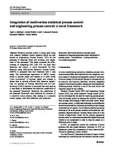
Neural network approach For many years humans have been trying to understand how the brain works with the hope that such knowledge would enhance our ability to implement machine intelligence; (artificial) neural networks are the outcome of such enquiries. In general, a neural network could be a pattern recognizer, similar in function to the classical, statistical (non-parametric) approach. A feature vector is input into the net and the output of the net categorizes the outcome into one of several classes; in this problem two classes are involved: shift in mean and shift in variance. The steps involved in the application of a neural network are: selection of a feature vector, selection of a network structure, training and implementation. A neural network consists of a large number of interconnected nodes which are nonlinear computational elements in a parallel processing structure. The weight given to each nodal connection evolves according to some preset learning criteria. The implicit knowledge of the net obtained during training is contained in the interconnection weights. There exists a variety of different structures and learning algorithms useful for neural network application. Within the context of the current problem, the feedforward network with the back-propagation error rule (under supervised learning) will be discussed. The back-propagation method has been shown to work well in pattern recognitions (Pao 1989). (A comprehensive introduction to such issues can be found in Lippman 1987, Runelhart and McClelland 1986). Figurel shows a typical feed-forward neural network consisting of several layers of nodes. Two 'visible' layers are input and output. These bracket other hidden layers.

Change structure in statistical process control

1657

Output Pattern

Output Layer

Wi,J,3

Second Hidden Layer

Wi,j,2

Downloaded by [Arizona State University] at 05:34 07 July 2014

First Hidden Layer

Wi,J,!

Input Layer

Input Feature or Input Pattern

Figure 1. Feed-forward neural network.

Each node in each layer is connected with each node in the succeeding layer, and those connections are unidirectional, towards the output layer. The function of hidden layer(s) is to map the feature vector into a different metric space with the hope that it will further assist the task of classification. There exist tradeoffs between having too few or too many hidden layers. If there is no hidden layer, this particular net is called a perceptron, known to behave as a linear separator (Rumelhart and McClelland 1986). A perceptron only works well in problems which are linearly separable, which is not the case here. Ifa net contains more hidden layers than are necessary it may introduce 'noise' into the net and also increase traning set size. The general rule of thumb for neural network structure is that the number of hidden layers should be either one or two (Lippman 1987). With two hidden layers the net can classify almost any complex region of clusters, as long as they are separable. The number of nodes in the input layer is directly determined by the size of the feature vector. The number of nodes in the output layer is determined by the number of different classifications desired. There are no general guidelines used to specify the 'optimal' number of nodes required in the hidden layer-this number appears to be highly problem dependent. Each node in each layer contains a threshold value. The difference between the threshold and the weighted input to the node is called the net input. The use of a threshold is to prevent oversensitivity to small, random disturbances. Each node also contains a corresponding activation function which is nonlinear and a monotonically increasing function of net input. The nonlinearity of the activation function is necessary in order to categorize clusters of pattern which are not separable into simple linear regions (Rumelhart and McClelland 1986). The value of a

1658

Y. Guo and K. J. Dooley

node's activation function is multiplied by the weights between the node to those nodes in the succeeding layer. Specifically, let:

f(-):

activation function

Wi,j,k: weight between i th node in (k -I) th layer to j th node in k th layer 7),k: threshold of thejth node in the kth layer Ij,k: net input to the j th node in the k th layer OiJ output of the i th node in the jth layer

nk : number of nodes in k th layer The net input and the output of the j th node in the k th layer is given by: ",,-1

ljk=

L (I¥;jk' Oik-d-7)k

(I)

Downloaded by [Arizona State University] at 05:34 07 July 2014

i= 1

(2)

Neurological research shows that the activation function for a brain cell (or neuron) is basically a step function with respect to a stimulus (Rumelhart and McClelland 1986). Because the step function is not differentiable, which is a desired characteristic for most training algorithms, the sigmoid function, which closely resembles the step function, is often used (Fig. 2): 1 f(x) = 1 +exp( -x)

(3)

The neural network can be trained by the back-propagation training algorithm, or generalized delta rule (Rumelhart and McClelland 1986). First, node weights and threshold values are initialized to random values; this helps prevent the net from being Step Activation Fuctlon

SlgmOld Activation F..met

f()

ron f(

a

Figure 2. Activation functions.

)

Change structure in statistical process control

1659

Downloaded by [Arizona State University] at 05:34 07 July 2014

trapped at a local extreme at beginning of training. Next, the feature vector, which is . defined as an abstraction of the most fitting description of the object of interest, is ' presented to the input, or zeroth layer. The vector is in hyperspace R" given the dimension of the feature vector is n. At the same time a prespecified output vector, containing the 'correct' or desired output given that input, is given to the output layer. The net feeds the feature vector data through the net to the output layer. The actual output vector is compared with the desired output. If a discrepancy exists, backward propagation begins. This backward error propagation is designed to modify the thresholds and weights in the direction so that the overall error will be minimized, according to a quadratic loss function. The optimization method used is a modified gradient technique for an . unconstrained optimization problem (Rumelhart and McClelland 1986). The amount: of change in a given weight is:

aE

t1W;jk=-'1aljkOik-l

(4)

where t1W;jk is the change in the weight between the i th node in the (k - 1)th layer and the j th node in the k th layer, '1 is a constant between 0 and 1and represents the learning rate, and E is the quadratic loss function to be minimized. U'k' is the output layer then:

aE

,

al = -(tij-Oik)!(Iik) jk

(5)

where t jk is the target value for the j th node in the output layer. If'k' is not in the output layer, then:

ee

-al = jt

(".+1 .L -ee al 1=1

W;jk+l

)!'(Ijk)

(6)

jl+l

Additionally, the 'momentum' of learning is sometimes controlled by an additional constant (x, also between 0 and 1, such that at iteration t the new change in weight is given by: (7) For multi-layer problems the backward-propagation algorithm may stop at a local extreme point, but in practice this rarely happens (Lippman 1987). By repeatedly presenting pairwise input feature vectors and the desired output vector to the net either the error rate will converge to the desired error level or training will not converge at all. Non-convergence can be caused by many possible situations, including: (a) poor choice offeature vector, (b) insufficient network structure given task complexity, (c)insufficient training, or (d) the nature of the problem is not tractable by the feed-forward and backward error propagation approach. Properly designed experiments help identify alternative configurations which overcome difficulties in (a), (b), or (c). While selection of feature vector elements can be accomplished formally, initial identification of possible elements is a matter of problem expertise. If all alternative configurations yield unsatisfactory results, (d) may be diagnosed and another pattern recognition approach needs to be tried. 3.

Bayesian discriminant function approach A Bayesian pattern recognition formulation can also be used to identify the change structure. Given the input feature vector X (same as zeroth layer of neural net), we desire to specify which class (category) it belongs to such that the average probability of

1660

Y. Guo and K. J. Dooley

error is minimized. Suppose further that we know the a priori probabilities of class y' occurring, Prob (cj ), where ci={ c 1 , ... , cR } , and the conditional densities p(Xlc). Bayes rule gives the posterior probability of cj by (Fukunaga 1972): p(Xlcj)prob (c) R

L P(Xlc;)Prob (c.)

(8)

i=l

Downloaded by [Arizona State University] at 05:34 07 July 2014

Class j is then chosen as the correct classification such that Prob (cjIX) is maximized. Because each computed probability using equation (8) has the same denominator, the decision is left unaltered if the denominator is eliminated. Likewise, the logarithm can be taken of the remaining function, yielding what is commonly referred to as the discriminant function (Duda and Hart 1973): Prob (cjl X) cx: log (pXlc)l+ log (Prob (Cj))

(9)

For Gaussian data the quadratic discriminant function (QDF) could be represented by (Dud a and Hart 1973): Prob (c) X) o; -(X -llyI j-I(X -Il)-Iog (IIjll+ 210g (Prob tcjl)

(10)

where Ilj and I j are the mean and covariance matrices of the feature vectors obtained from the training data corresponding to class j. IfI j is essentially identical for all different classes, the QDF can be further simplified into the linear discriminant function (LDF) (Duda and Hart 1973): (11)

In the case here,j = 2 since the two classes are shift in mean and shift in variance. Since we cannot assume equality of I for our problem, QDF and LDF will be experimentally compared in section 5.1. One may question whether, for a particular problem, it is safe to assume normality of the feature vector. In many cases the distribution of a particular statistic in the feature vector is known to be normal or known to be from a distribution which can be approximated by normality following some nonlinear transformation. In other cases where the distributional characteristics of an element within the feature vector are not known, normality is usually assumed. In general the LDF/QDF is fairly robust to nonnormality for few elements in the feature vector if the dimension of the vector is relatively high (Anderson 1984). In the case where non-normality is extreme performance of the classification will be poor and non-parameteric approach may need to be used. In the case presented here some of the feature vector elements, such as a sample variance, are not normal. This does not appear to deter from the good performance, however, if the LDF/QDF approach. In order to compute the probabilities given in equations (10)and (11) Iljand I j must be estimated for each class j. The maximum likelihood estimators of mean vector and covariance matrix for each class j are j are (Anderson 1984):

f1j =

MiX ..

L---..!L

i~IMj

(12) (13)

Change structure in statistical process control

1661

The a priori probabilities Prob (c) can be estimated by experience or historical data analysis; if they are set as '1IR' (i.e. non-informative prior) as they are in this problem, they can be eliminated from equations (10) and (11).

Downloaded by [Arizona State University] at 05:34 07 July 2014

4. Neural network and Bayes decision approach to change structure identification 4.1. Description of the problem The process under consideration is one which yields a univariate quality characteristic which, when sampled at equal intervals of time, yields a normally and independently distributed random variable y, with constant mean and variance; without loss of generality we can assume that the process mean is zero and variance is one. At some time t* the process experiences a special cause which has one of the two following effects: Mean change: y, = k + e, Variance change: y,=ce, where t > t* and e, is a N(O, I) variable. Identification takes place at time T, when the process change is detected-thus it is assumed that no data is available after the process change has been detected by the appropriate statistical method. The justification of using this more abstract approach is that it makes the research results problem independent. Thus, as long as the actual ' process output data can be filtered to a N(O, I) variable, the approaches that are presented here will yield similar results in actual application. Such filtering, in the independent Gaussian case, is as simple as subtracting the sample mean and dividing by the sample standard deviation. In more complex signals, time series modelling can be used to extract the deterministic and stochastic dynamics from the signal, therefore, change detection and analysis can proceed with the model residuals (Dooley and Kapoor 1990a). In order to simplify the study, only positive shifts in the mean (i.e. k>O) will be considered- this does not cause a loss of generality. Additionally, only increases in the process variance (c> I) will be considered; Dooley and Kapoor (1990) showed that there is almost no 'overlap', as reflected by test statistic behaviour, between the variance decrease and a mean shift, therfore, the problem of a variance decrease is considered trivial. The problem of a mean shift versus a variance increase, however, is not (Dooley' and Kapoor 1990a). One can see that 'k' represents the magnitude of the mean shift in terms of standard deviations, and that 'c' represents the multiplicative increase in standard deviation. Thus, after the change point t*, y, is distributed normally with mean k and standard deviation one when the mean shifts, whereas y, is distributed normally with zero mean and standard deviation c when the variance shifts. Next, a decision must be made regarding the selection of appropriate test statistics to be used to detect the process change. Because of their sensitivity to process changes and ease of computation the cusum chart (Van Dobben de Bruyn 1968) and rnosumsquared chart (Bauer and Hackl 1980) were chosen. The cusum chart is used to specifically test the hypothesis that the process mean has not shifted from zero. The test parameters 'K' and 'h' determine the rejection regions of the test and consequent sensitivity. A computationally effectiveway of implementing the cusum chart is given in

Y. Guo and K. J. Dooley

1662

Van Dobben de Bruyn (1968),where positive and negative sums are plotted over time. Assuming zero mean and unit variance, the cusum chart uses the following equations: So(+ )=So( - )=0 S,( +)= Max(O,S'_I( +)+ y,-K) S~ -

(14)

)=Min(O,S'_I( -)+ y,+K)

A change in the process is noted when S,( + ) is greater than h, or S,( - ) is less than - h. The mosum-squared test is based on the sum of squares of a moving window of data, and is thus related to a Chi-squared test (Bauer and Hackl 1980). At each time t we calculate (assuming zero mean and unit variance):

Downloaded by [Arizona State University] at 05:34 07 July 2014

(15) The sum of squares is calculated using N( = t 2 - t I + I) residuals, and N is kept constant so that the corresponding rejection region is also constant. Average run length behaviour can be used to establish an appropriate rejection region. In the experiments to follow, the test stastic parameters are: h is 6·0 and K is 0·5 for the cusum chart, and N is 25 and the rejection limit for SSQ, is 52·6719; these correspond to an average run length of about 1000 when no process change occurs (i.e. oe error rate of 0·001). Selection of test parameters which yield better sensitivity would also increase the rate of false alarms. It should be noted that as test sensitivity is increased, the change structure identification problem becomes more difficult because as changes are detected more quickly, there is a smaller amount of data. available to draw conclusions upon. In order to illustrate the change structure problem simulation data is shown in Figs 3 and 4. Both show sets of data which undergo a change in structure at sample 26. In Fig. 3, the mean shifts from 0 to 0·5 and is detected at sample 55; in Fig. 4, the standard

Samples Numkr

Figure 3. Mean shift in process at sample 26.

Change structure in statistical process control

1663

.,

Downloaded by [Arizona State University] at 05:34 07 July 2014

·2

-3+-_~~

__

o

__-,-__

-,-_~~

10

20

----':'-----_~_~~_..---j

30

40

SampleNumber

Figure 4. Variance shift in process at sample 26.

deviation of the process increases from 1·0 to 1·5 and is detected at sample 37. The detections are done by applying the two tests, namely the cusum and mosum-squared tests, that are given above. When either test (or both) signals a change, it is at this point that the structure identification methods would be invoked.

4.2. Feature vector selection There are many different elements which could be used to construct an appropriate feature vector for this problem. We shall discuss these possibilities and then compare these selections in the following section. Since there are only two types of change structures being investigated, and because the sample mean and sample variance are sufficient statistics for estimation ofthe mean and variance of the population, functions of these statistics are natural candidates for elements offeature vector. Because of unknown change point, however, these estimates may be contaminated, i.e. data used in estimation may come from two populations. From statistical theory the counterparts of the sample mean and variance which are somewhat robust to contaminated data are the sample median and range, therefore these will be investigated. Additional, the test statistics themselves (S,( +), S,(- ), and SSQ,) are also candidates. Finally, the feature vector could be (partially) composed of the actual raw data. 4.3. Training Since one does not have prior knowledge of the relative occurrence of mean shifts versus variance shifts, a training set is established using a non-informative prior, i.e. equal number of mean shift cases and variance shift cases are presented. For the neural network approach the training period is considered finished when either the relative error rate is less than a specified tolerance value or a certain number of training. iterations has been reached. This same set of test data is used for estimating the mean and covariances required in equations (12) and (13), thus allowing a fair comparison between the Bayesian discriminant functions and the neural networks.

1664

Y.Guo and K. J. Dooley

5. Experimental results

Downloaded by [Arizona State University] at 05:34 07 July 2014

5.1. Preliminary results Before comparisons can be made between the neural network and pattern recognition approaches, the performance of both must be investigated so as to determine the best set of 'operating conditions'-this includes selection of the: (a) feature vector, (b) training pattern to be used, (c) number of layers in the neural network, (d) number of nodes in the neural network, and (e) type of discriminant function to be used. The following describes the conclusions drawn from these trial experiments. (The detailed descriptions of these tests can be found in (Guo and Dooley

1990).) For neural network parameter selection, the following conditions apply unless otherwise specified: two hidden layers; a linearly decreasing learning rate with momentum of 0·7; and training is stopped and the network is considered complete either when the relative error rate from iteration i to i + I is less than I % or 10 000 iterations have been reached (in most cases the first condition was met after 2000 iterations). The selection of these comes from several sets of experiments which examined other alternative designs (Guo and Dooley 1990). As mentioned in section 4.2, there are many candidates for possible representation in the feature vector. After many combinations were tested the following vector was decided upon: S.,( +), s.,( -), SSQT (the test statistics), Yn YT-\' YT-2' YT-3' YT-4 (the five data points available prior to change detection) and the sample mean and variance statistics using data from the data windows {T - 5, T - 9}, {T - 10, T - 14}, T -IS, T -19}, and {T - 20, T - 25}, respectively. Thus the chosen feature vector has dimension J 6. Other combinations that did not prove as satisfactory in terms of their performance in structure identifications were feature vectors which: (a) eliminated the sample statistics, (b) eliminated the actual raw data, (c) only included the raw data, and (d) substituted the median and range within the chosen data windows instead of the mean and variance. All choices of the final alternative design came after appropriate statistical comparisons. Given a feature vector, there are many different ways that one can go about training the neural network to distinguish between mean and variance shifts. The simplest approach is to train at a single magnitude of shifts, say k = 1·0 for a mean shift and c = 2·0 for a variance shift. Under this arrangement it was found that the neural network only performs well when it is tested at the same magnitude it was trained at. Thus, if you train it to distinguish at small magnitudes, it does poorly at large magnitudes, and vice versa. This is not acceptable, since under most circumstances the actual process may experience changes representing a whole range of magnitudes. Next, several 'sweep' training patterns were tried. In this arrangement the net was trained at, for example, {k =0·25,0·5, 1·0, 1·5,2·0, and c = 1·25, 1·5,2·0,2·5, 3·0}. Results were compared (using a paired t-test approach) with the first training pattern and found to be significantly better at the 0·01 significance level. Finally, the net was trained via a 'uniform sampling' approach. Training cases were alternated between mean and variance shifts, and at any given time the magnitude that was simulated was chosen from a uniform distribution. For mean shifts 'k' was chosen in the range [0·25,2·0] and for variance shifts 'c' was chosen in the range [1·25,3·0]. A paired t-test showed that there was no difference between the sweep and uniform sampling training patterns for mean shifts, but that the uniform sampling approach yieldeda significantly lower error rate, for variance changes. The uniform sampling method also yields approximately equal average error rates for both mean shifts and variance shifts, which is an attractive property.

Downloaded by [Arizona State University] at 05:34 07 July 2014

Change structure in statistical process control

1665

Given a two hidden layer net, experiments were run to determine how many nodes in each of the two layers needed to be present in order to get optimal performance. While no specific response surface strategy was used to explore the parameter space, it did appear as if there existed an 'optimal' number of nodes that was neither small nor large. Experiments with too few nodes in the hidden layers proved to yield unsatisfactory performance; experiments with too many hidden nodes (for example, 48 nodes in the first hidden layer and 144 in the second hidden layer) did not converge during training. The optimal size (lowest error rate among those combinations tested) was a net which had 48 nodes in the first hidden layer and four in the second hidden layer. Next, experiments were run to determine whether a net with two hidden layers needed to be used, or whether a single hidden layer would suffice. For the two hidden layer net, 48 and four nodes were used; for the one hidden layer net, four nodes were used. Paired comparison showed no difference in performance for the mean shift case, but significanty better performance (at significance level of 0'01) for the two hidden layer net for variance shifts. In conclusion, the best net appeared to be one which: (a) contained both raw data, summary statistics, and test statistics in the feature vector, (b) was trained across a wide spectrum of possible change mangitudes, (c) had two hidden layers with 48 and four nodes, respectively. The final structure used in this research is an input layer of 16 nodes; first hidden layer of 48 nodes; second hidden layer offour nodes; an an output layer of one node. Because there are two classes, mean and variance shift, an output of '0'0' corresponds to mean shift and an output of '1'0' corresponds to variance shift. The neural network configuration used here naturally forces the output to be close to 0·0 or 1·0 (Runelhart and McClelland 1986). Finally, testing was done to see whether the problem could be addressed using the simpler linear discriminant function, or ifthe quadratic function was needed. A training set of 2000 feature vectors, generated in the same manner discussed above, was used to form the mean vector and covariance matrix needed by equations (12) and (13). Statistical comparison of the LDF and QDF showed that there was no difference in performance between the two for mean shifts, but that the QDF performed significantly better (at a significance level of 0'01) than the LDF for variance shifts.

5.2. Comparison of the methods In this section we report on and compare the performance of the neural-network and QDFapproaches. Because no previous work in this area exists, it was also decided to investigate the performance of two other, simpler heuristic methods. These heuristic methods were chosen such that they most closely relate to how the change structure identification problem is informally addrressed in practice. The training pattern, net and QDF parameters chosen are those described in the previous section. The first heuristic, H 1, assumes that the data coming from the process is being analysed on a Shewhart control chart for individuals, or an X-moving range charge. Given individual data that is not amenable to natural subgrouping, as is the case here, this chart would likely be the practioner's tool of choice. If the moving range chart alone signals a process change, a variance shift is declared. If the X-chart signals a change either alone or simultaneously with the moving range chart, a mean shift is declared. In both charts a change is signalled when a point is beyond the respective control limits.

Y. Guo and K. J. Dooley

1666

Error rate k

c

0·25 0·50 0·75 1·00 1·25 1·50 1·75 2·00

Downloaded by [Arizona State University] at 05:34 07 July 2014

(Average) 1·50 1·75 2·00 2·25 2·50 2·75 3·00

(Average) Combined Average

NN

QDF

HI

H2

0·010 0·009 0·019 0·023 0·038 0·078 (}I 18 0·182 0·060

0·057 0·007 0·003 0·005 0·013 0·023 0·038 0·056 0·025

0·491 0·411 0·368 0·294 0'241 0·210 0·207 0·193 0·302

0·056 0·011 0·007 0·012 0'023 0·031 0·031 0-080 0·031

0·084 0·069 0·063 0·055 0·044 0·045 0·037 0·057

0·118 0·101 0-089 0·079 0·076 0-075 0-071 0-087

0·314 0·359 0·394 0'441 0·456 0-467 0-492 0·418

0·222 0·205 0·198 0'186 0-174 0·174 0·156 0·188

0·058

0-056

0-360

0·109

Table 1. Performance of methods which identify change structure.

The second heuristic, H2, also assumes that change structure is identified directly from the test statistics, but that a more complex and sensitive approach is used to detect process changes, namely, the cusum chart and mosum chart. If the cusum chart signals a change, a mean shift is declared. If the mosum chart signals a change, a variance shift is declared. If both signal a change simultaneously, previous research (Dooley and Kapoor 1990a) has shown the most likely change structure to be a variance shift, Changes are signalled by both tests in the same manner as described in section 4.1. Table I shows the results ofthe comparative tests; 'error rate' refers to an incorrect classification, i.e.a method said 'mean' when it was 'variance', or vice versa. Error rates are based on 1000 trials at each category. To be specific, for mean changes there are eight different magnitudes k under investigation, where k ranges from 0·25 to 2·0 with an increment 0·25. For variance changes there are seven different magnitudes c, where c ranges from 1·5 to 3·0 with increment 0·25. This seems to be a reasonable range of magnitudes encountered in practice. Shifts smaller than this range are very difficult to detect, and thus diagnose. Shifts larger than this range can be detected extremely quickly (in less than fivesamples usually) and thus make change structure identification relatively impossible. At each magnitude for mean and variance changes, four different methods, namely, neural network, quadratic discriminant analysis, heuristic I qnd heuristic 2, are compared. At each magnitude 1000 trials are run. Each trial consisted of generating a stream of y, values with a change of given magnitude occurring at t = 26. When the change was detected, the feature vector of data was constructed (as described in the previous section) for the neural network and QDF, and the four classification mechanisms were invoked. Performance of incorrect or correct classification was noted and represented as average error rate over 1000 trials in Table I. Note that these 'test trials' are completely separate from the previous training trials.

Downloaded by [Arizona State University] at 05:34 07 July 2014

Change structure in statistical process control

1667

First, let us examine the neural network and QDF approaches. The average error rate for mean shifts is extremely low for both, at 6% for the neural network and 2'5% for QDF. For variance shifts the neural network performs better, yielding 5·7% errors as opposed to 8'7% for QDF. Overall error rates for the two are essentially identical, at 5·85% for the neural network and 5'6% for QDF. For the simple HI heuristic, the average error rate for mean shifts is 30% while for variance shifts it is 42% (only slightly better than random guessing). The main reason for this poor performance is the inability to distinguish change structure when both the X and moving range chart simultaneously signal a special cause. Average error rate for H2 for mean shifts is 3·2%, which is quite good, but for variance shifts it is 18'8%, which is considerably higher than that of the neural network or QDF. The overall error rate for H2 is 10'95%. For these four approaches six separate pairwise t-tests are conducted for the mean shifts and variance shifts. The purpose of these tests is to see whether or not there is a significant difference in performance between any two approaches. Performance is paired at each separate magnitude. Due to multiple testing criteria via the Bonferroni inequality, the significance level for each comparative test is set at 0·0017 so that the overall type I error is 0·01. There is no significant difference for the error rate of the mean shifts among neural network, QDF and H2 approaches; they all are statistically significant better than HI for mean shifts. Even though QDF and the neural network appear to be different in terms of their overall average (0'025 versus 0,060), the pairwise differences have too high a variability to show statistical signficiance. For variance shifts the neural network performs significantly better than QDF, QDF performs better than H2, and they all perform better than H I. Thus, in summary, the tests reveal that, while the neural network and QDF approaches are relatively similar, the neural network approach is superior in dealing with variance changes, and also has the attractive feature of yielding equal average error rates for both mean and variance changes (i.e. it is unbiased).

·1

·2

10

20

Sample Number

Figure 5. Plot of assay values over time.

30

Downloaded by [Arizona State University] at 05:34 07 July 2014

1668

Y. Guo and K. J. Dooley

5.3. Example As an example a data set (Hawkins 1987)of assay values is investigated. The data represents laboratory measurements on the concentration of a precious metal contained in batches of feedstock. A change in the mean of the assay values may represent drifts in equipment, measurement errors, and changes in the source, while a change in variability may represent contamination of the samples and/or source or handling errors. Data are monitored via the cusum and mosum charts discussed in section 4. The first 20 samples are used to estimate the mean and the variance of the stable process. A change is indicated by the cusum chart at sample 31. A plot of the raw data is shown in Fig. 5; numbers have been standardized to ensure the proprietary nature of the process. One can see from the plot, with the aid of data collected well after the change occurred, that the true change structure is a shift in the mean. The challenge however is to identify the change structure with only samples Yl through Y31. The feature vector which is used for change structure identification, as described in section 5.1, has 16 elements. First, there are the test statistics S31( +), S31(-), and SSQ31' which have the values of 6·07,0·00, and 47·38. Next, the five most previous residuals (data have already been standardized in this case) Y31' Y30' Y29' Y28' and Y27' which have values of 0·97, 0·40, 4·13, 1·24, and \·68 respectively. Finally, the sample mean and standard deviation is calculated for four windows of residuals, each window being of size five, ending at sample 26. Thus the sample mean and standard deviations are calculated for the residual sets {Y7·· ·Yl d, {YI2·· ·YI6}' {YI7·· ·Y21}, and {Y22···Y26}· The neural network used to identify the change structure is the same as tested previously; using the feature vector as input, the output node contains the value 0·07, where '0' corresponds to a mean change and '1' to a variance change. Thus, the neural network successfully identifies the change structure as a shift in mean, and diagnostic efforts can be focused on those phenomena which cause such a structural shift.

6. Summary The change structure identification problem is an important aspect of diagnosis in a quality improvement environment. Given the occurrence of a special cause, the diagnostic search can be reduced in length if one has knowledge of whether the process change was a shift in mean or variability, and corresponding knowledge of which process factors affect mean and variability of output. This paper presented neural network and quadratic discriminant function (QDF) approaches to solve this statistical classification problem. . Monte Carlo simulation experiments were used to test the performance of the two proposed methods. Tests were done at eight different magnitudes of mean shifts and seven magnitudes of variance shifts, with 1000 trials at each magnitude. The average success rate across all magnitudes for identifying a mean shift was 94% for the neural network and 97·5% for QDF. For variance shifts the neural network performs better, yielding 94·3% correct identification as opposed to 91·3% for QDF. The overall success rates for the two are essentially identical, at 94·\5% for the neural network and 94·40% for QDF. Both performed (statistically) significantly better than two other simpler heuristic methods which closely reflect how the problem is currently handled in practice. Thus adoption ofthis approach could improve evaluation of changes detected in statistical process control schemes, thus enhancing diagnostic capabilities and furthering process improvement efforts.

Change structure in statistical process control

1669

Downloaded by [Arizona State University] at 05:34 07 July 2014

References ANDERSON, T. W., 1984, An Introduction to Multivariate Statistical Analysis, 2nd edition (New York: John Wiley & Sons). BAUER, P., and HACKL, P., 1980, An extension of the MOSUM technique for quality control. Technometrics, 22 (1), 1-7. BERGER, J. 0.,1985, Statistical Decision Theory and Bayesian Analysis, 2nd edition (New York: Springer-Verlag). DOOLEY, K., and KAPOOR, S., 1990 a, An enhanced quality system for continuous manufacturing processes, Part 1: Theory. Journal of Engineering for Industry, 112 (1), 57-62. DooLEY, K., and KAPOOR, S., 1990b, An enhanced quality evaluation system for continuous manufacturing processes, Part 2: Application, Journal ofEngineeringfor Industry, 112 (I), 63-68. DUDA, R. 0., and HART, P. E., 1973, Pattern Classification and Scene Analysis (New York: John Wiley & Sons). FUKUNAGA, K., 1972, Introduction to Statistical Pattern Recognition (New York: Academic Press). Guo, Y., and DooLEY,K. J., 1990, The application of neural networks to a diagnostic problem in quality control. Proceedings of ASME-WAM: Monitoring and Controlfor Manufacturing Processes, 111-122. HAWKINS, D., 1987, Self-starting cusum charts for location and scale. The Statistician, 36,299315. LIPPMAN, R., 1987, An introduction to computing with neural nets. IEEE ASSP Magazine, 4-22. PAO, Y. H., 1989, Adaptive Pattern Recognition and Neural Networks (London: Addison-Wesley). RUMELHART, G., and MCCLELLAND, J. (Eds.), 1986, Parallel Distributed Processing (Cambridge, MS: MIT Press). VAN DORREN DE BRUYN, C. S., 1968, Cumulative Sum Tests (London: Hafner Publications).