Identifying and Predicting Economic Regimes in Supply Chains Using Sales and Procurement Information Frederik Hogenboom
Wolfgang Ketter
Rotterdam Sch. of Mgmt. Erasmus University Rotterdam
Rotterdam Sch. of Mgmt. Erasmus University Rotterdam
Erasmus Sch. of Econ. Erasmus University Rotterdam
Computer Science and Engr. University of Minnesota
Carlson Sch. of Mgmt. University of Minnesota
[email protected] Uzay Kaymak
[email protected]
[email protected] John Collins
[email protected]
ABSTRACT We investigate the effects of adding procurement information (component offer prices) to a sales-based economic regime model, which is used for strategic, tactical, and operational decision making in dynamic supply chains. The performance of the regime model is evaluated through experiments with the MinneTAC trading agent, which competes in the TAC SCM game. We find that the new regime model has a similar overall predictive performance as the existing model. Regime switches are predicted more accurately, whereas the prediction accuracy of dominant regimes is slightly worse. However, by adding procurement information, we have enriched the model and we have further opportunities for applications in the procurement market, such as procurement reserve pricing.
Categories and Subject Descriptors I.2.11 [Artificial Intelligence]: Distributed Artificial Intelligence; K.4.4 [Computers and Society]: E-commerce
General Terms Algorithms, economics, theory
Keywords Economic regimes, machine learning, supply chain management, TAC SCM, trading agent
1.
Jan van Dalen
Erasmus Sch. of Econ. Erasmus University Rotterdam
INTRODUCTION
Because of the extremely competitive character of today’s markets, it is important to gain insight into the dynamics of supply chains and to research supply chain optimization possibilities, both for individual elements in the chain, as
Permission to make digital or hard copies of all or part of this work for personal or classroom use is granted without fee provided that copies are not made or distributed for profit or commercial advantage and that copies bear this notice and the full citation on the first page. To copy otherwise, to republish, to post on servers or to redistribute to lists, requires prior specific permission and/or a fee. ICEC ’09, August 12-15, 2009, Taipei, Taiwan c 2009 ACM 978-1-60558-586-4/09/08 ...$10.00. Copyright °
[email protected] Alok Gupta
[email protected]
well as for the chain as a whole. For instance, in correctly predicting future market conditions (economic regimes [7]) lie competitive advantages, because one can anticipate on upcoming scarcities or oversupply in the sales market by adjusting procurement policies and sales prices in advance. This can save for instance storage costs, and increase profits. Therefore, one could benefit greatly from being able to make tactical and strategic decisions in an uncertain market, based on predicted and identified economic regimes. Combining techniques from computer science with economic theory to solve problems in economic environments contributes to novel approaches to existing problems. Ketter introduced an economic regime model, which is based on sales information [7]. This model can be applied to any market situation and to simulated markets. However, procurement information has not been used sofar for identifying and predicting regimes, despite the fact that this information could be valuable for determining economic regimes, since it captures certain market characteristics. For instance, an increase in the amount of components sold in the procurement market could indicate an expected scarcity, as manufacturers are building stocks. We present an extension to the regime model as introduced by Ketter, which is implemented in the MinneTAC trading agent [4]. We investigate the effects of adding procurement information to this model. The performance of the regime model is evaluated through experiments on the quality of regime probability predictions, and checking correlations with existing market conditions. The MinneTAC trading agent has competed for several years in the Trading Agent Competition for Supply Chain Management (TAC SCM). TAC SCM is an annual international competition for designing trading agents for a simulated personal computer (PC) supply chain [3]. TAC SCM has attracted researchers from all over the world, because of its characteristics. The game environment is designed in such a way that it contains many characteristics that can be found in real-life supply chains, such as the behavior of unpredictable opponents and interdependent chain entities. The simulated supply chain of the TAC SCM game offers many research opportunities into various subjects, such as price setting strategies and prediction strategies for competitor behavior or market characteristics and developments. Because of its complexity and size, new subcompetitions of the TAC SCM game have emerged over the
past few years, which focus on specific parts of supply chain management, such as optimizing price predictions, which is the main activity in the TAC SCM Prediction Challenge, or the TAC SCM Procurement Challenge. The supply chain of the TAC SCM games is simplified, so that it only consists of suppliers, manufacturers, and customers. In total, sixteen types of PCs are traded, which can be classified into three market segments: the low-, mid-, and high-range products, mainly differentiating in product price. Products across the overall market share parts. In TAC SCM, artificial trading agents compete with each other in groups of six in two markets: the sales market for customer orders and a procurement market for computer components. The winner of each round of the game is the agent that maximizes profits. Each game simulates 220 days, which take fifteen real seconds each. Each day, agents have to perform numerous tasks. The trading agents place bids, buy components from suppliers, ensemble PCs in their factories, and sell products to customers (see Figure 1).
Figure 1: Schematic overview of the basic concepts of the TAC SCM game. Even though trading agents are human-created, human intervention is not allowed during a game, and thus agents rely on their own calculations and predictions. The TAC SCM takes care of generating supply and demand, generating market reports every twenty days with information about shipments and orders, and providing banking, production, and warehousing services. The paper is organized as follows. First, we continue with Section 2, which introduces the economic regime model which is currently used in the MinneTAC agent. Subsequently, we define a new regime framework based on sales and procurement information in Section 3. This new model is evaluated in Section 4. Finally, conclusions are drawn and future work is suggested in Section 5.
2.
BACKGROUND AND RELATED WORK ON REGIMES
MinneTAC’s sales decisions are largely dependent on the regime identification and prediction modeled in the regime model [11]. Every day, for each individual product, the probabilities of current and future economic regimes are determined. Many decisions are based upon current and expected
regimes and their directly associated price density forecasts. With the help of the current and future price density we are able to predict market prices, market price trends, and the customer acceptance probability for specific offers. Regimes are used for both tactical and strategic decisions, such as product pricing and production planning. The regimes in the TAC SCM game can be considered as a set of characteristics which apply to a certain period of days. The identification and prediction of regimes is done so that different behavior can be modeled for different situations, which is also referred to as a switching model. The agent’s problems can be solved differently, depending on their (regime) classification, thus influencing the accuracy of the agent’s predictions and the amount of profit made. Regimes are used in multiple contexts. One can apply regimes in political and economic contexts. In general, a regime refers to a set of conditions. In economic context, regimes are also referred to as business cycle phases. These phases are commonly used in macro-economic environments, as is the case in [16]. However, in [7], regimes are applied in the micro-economic environment of the TAC SCM game. This makes sense, since an economic environment is simulated and one can capture (economical) characteristics in economic regimes, enabling an agent to reason (i.e., make tactical and strategic decisions) based on certain market conditions. Other applications of regimes can be found in electricity markets. These markets often are oligopolies, which is also the case in TAC SCM. Becker et al. and Mount et al. both model spikes in electricity prices as a regimes switching model, based on Markov switching models [2, 15]. Over the past decades, research has been into identifying and predicting regimes, but also into regime changes. Regime changes are important events in time series, in which one can obtain strategic advantage if they are predicted or identified correctly. Recently, Massey and Wu [13] emphasize this importance of the ability to detect and respond to regime shifts, as it is critical to economic success. If these shifts are not detected, this could lead to lower profits. Also, Massey et al. elaborate on the causes of under- and overreaction to (predicted) regime shifts. The foundation of research into regime shifts lies in 1989, when Hamilton published a paper about modeling regime changes using postwar U.S. real GNP as input [5]. Hamilton used Markov matrices to observe these regime shifts, by drawing probabilistic inference about whether and when they may have occurred based on the observed behavior of series. The algorithms implemented in the regime model implemented by the MinneTAC agent, which identifies and predicts economic regimes, are based on economic theory and incorporate some adapted techniques. The model’s regimes are identified as extreme scarcity, scarcity, a balanced situation, oversupply, and extreme oversupply [7]. As stated by Ketter, five regimes are used. We define the regime set as: R = {ES, S, B, O, EO} .
(1)
Each day of the game, the regime probability distribution is determined and a regime prediction is made. Thus, each regime Rk in set R ∀k = 1, 2, . . . , M (where M = 5) has a certain likelihood to hold as dominant regime. The regime probabilities in set R sum up to 1 and the regime with the highest probability is considered as the dominant regime.
Currently, the regime model identifies and predicts economic regimes based on yesterday’s normalized mean (sales) price [9] for an arbitrary day d, which is also referred to as npd−1 , as well as on quantities. Also, for some predictions, the entire history of normalized mean sales prices is used. The mean price is defined as the mid-range price. The problem is that in supply chains, data for the day itself is not available, and thus identification is done based on historical information, whereas prediction is done for day d up to planning horizon h (usually twenty days). The data the model is based on is normalized, as normalization enables easy computing. The range of the variable is fixed and thus known beforehand. Furthermore, it allows for machine learning across markets, i.e., over different products, which can be compared qualitatively, and it enables whole market forecasts. Regime identification is currently done by offline and online machine learning. Offer acceptance probabilities associated with given product prices (approximated using a Gaussian Mixture Model [17]), derived from observable historical and current sales market data, are clustered offline using the K-Means algorithm [12], which yields distinguishable statistical patterns (clusters). These clusters are labeled with the proper regimes after statistical research using correlations. Regime probabilities, which are indicative of how market conditions are, are determined by calculating the normalized price density of all clusters, given sales prices. There are several techniques for predicting regimes, each of which is most suitable for a specific time span. Today’s regimes can be predicted based on exponentially smoothed price predictions, as extensively elaborated in [10]. Shortterm regime prediction for tactical decision making is done by using a Markov prediction process. This process is based on the last normalized smoothed mid-range price. To this end, Markov transition matrices, which are created offline (i.e., not in the game) by a counting process over past games, are being used. Long-term regime prediction is done by using a Markov correction-prediction process. This process is almost equal to the short-term regime prediction, but is based on all normalized smoothed mid-range prices up and until the previous day, instead of just the last normalized smoothed mid-range price.
3.
EXTENDING THE REGIME IDENTIFICATION AND PREDICTION PROCESS
As there is no procurement information used in the regime model that is discussed in the previous section, we introduce an extended version of the regime model as introduced by Ketter et al. [11], using a simple model to illustrate the different computational steps. Our model differentiates from the model introduced in [11] in the fact that it is based on procurement information, and not solely on sales information. We apply the information gain metric [1] to a data set containing procurement information on prices, quantities, offers, orders, and requests for quotation gathered from historical game data1 in order to be able to deter1
Data set contains 2007 Semi-Finals games played on the SICS tac5 server (IDs: 9321–9328), 2007 Finals games played on the SICS tac3 server (IDs: 7306–7313), 2008 Semi-Finals games played on the University of Minnesota’s (UMN) tac02 server (IDs: 761–769), and 2008 Finals games played on the UMN tac01 server (IDs: 792–800).
mine which procurement variable adds the most information to the model. The next section continues with discussing the information gain metric.
3.1
Information Gain
The information gain is an entropy-based metric that indicates how much better we can predict a specific target by knowing certain features. When applied to our model so that the metric fits our needs, the dominant regime is selected as target variable and several procurement variables are used as features. According to Mitchell [14], the entropy is a commonly used measure in information theory, which characterizes the purity of an arbitrary collection of examples. Let W be a collection of game results. Then, numW is the number of possible values of W (i.e., regimes) and P (w) represents the probability that W takes on value w. Assuming a uniform probability distribution, P (w) is equal to the proportion of W belonging to class w. The entropy of a collection of game results, entropy (W ), is defined as entropy (W ) =
numW X
−P (w) log2 P (w) .
(2)
w=1
When we set V to be an attribute (procurement variable), numV the number of possible values of V , P (v) the probability that V takes on value v, and P (w|v) the probability that W takes on value w (given v), the entropy of a collection of game results W given a specific attribute V , entropy (W |V ), is defined as entropy (W |V ) = ÃnumW ! numV X X P (v) −P (w|v) log2 P (w|v) . v=1
(3)
w=1
With (2) and (3), the amount of information gained on outcome W from attribute V , gain (W, V ), can be calculated as gain (W, V ) = entropy (W ) − entropy (W |V ) .
(4)
Here, the entropy of a collection of game results W given an attribute V is subtracted from the entropy of W . Table 1 follows from the application of the information gain metric to several procurement variables using our data set. Note that the higher the score, the more information the variable adds to the model. Variable Offer price Order price RFQ lead time RFQ reserve price Ratio orders / offers Order quantity RFQ quantity Demand Offer quantity
Gain 0.7393 0.5400 0.5106 0.4909 0.4555 0.4310 0.3901 0.3833 0.3174
Table 1: Information gain scores for several procurement variables. The latter table shows that component offer prices (recalculated on a per-product basis) are most likely to improve the predictive capabilities of the regime model. Therefore,
we add these component offer prices, to which we refer to as op, to the existing regime model. These prices result from all requests for quotation in a TAC SCM game.
3.2
Regime Model Variables
As both regime identification and prediction are based on normalized sales prices, this section introduces a mathematical formulation of the normalized price np for product g, npg , on day d. The normalized price is calculated as npg =
asmCostg +
priceg PnumPartsg j=1
nomPartCostg,j
,
(5)
using the product price priceg , the product assembly costs asmCostg , and the nominal manufacturing costs for each component j belonging to product g, nomPartCostg,j , respectively. The estimated normalized mean price, which is used for regime identification and prediction, can be volatile and lacks information on trends. Therefore, (exponential) smoothing can be applied, resulting in yesterday’s exponentially smoothed normalized minimum and maximum prices, i.e., n f pmin f pmax d−1 and n d−1 . Equations (6) through (8) show how the exponentially smoothed normalized minimum prices are calculated, using a Brown linear exponential smoother, where α is a smoothing factor determined by a hill-climbing procedure. 0
0
min n f pmin f pmin d−1 = α · npd−1 + (1 − α) · n d−2 , 00 n f pmin d−1
n f pmin d−1
= α·
0 n f pmin d−1
+ (1 − α) ·
= 2·
0 n f pmin d−1
00 n f pmin d−1
−
00 n f pmin d−2
.
(6) ,
(7) (8)
Here, two price components are smoothed separately, after which both components are combined. This way, changes in the mean and trend can be captured. Brown linear exponential smoothing is applied, since the trend as well as the mean vary over time. The calculation of n f pmax d−1 is done by analogy with (6) through (8). Using the equations we have introduced previously, yesterday’s exponentially smoothed normalized price on an arbitrary day d can be calculated. This is done by averaging yesterday’s exponentially smoothed normalized minimum and maximum prices: n f pmin f pmax d−1 + n d−1 n f pd−1 = . (9) 2 We extend the regime model with the mean component offer price op for product g, opg , on day d, such that PnumS PnumCg opg,s,c c=1 s=1 opg = , (10) numOpg where numS refers to the number of suppliers, numCg refers to the number of components for product g, and numOpg represents the number of entries of the procurement variable. Thus, the mean component offer price is calculated by means of a counting process over all component prices. Because we would like the variable to include some information about other preceding days as well, so that it represents a trend instead of an event, we apply an exponential smoother to the variable. The smoothed value of yesterday’s product-based component offer price, of pd−1 , is calculated as shown in (11), where β represents a smoothing factor and is determined using a hill-climbing procedure: of pd−1 = β · opd−1 + (1 − β) · of pd−2 .
(11)
Smoothing is done by taking a certain percentage of yesterday’s value of op. Then, the remaining percentage is taken of the previous (smoothed) value of variable op, i.e., the day before yesterday’s value, after which both values are added. This is a less complex way of smoothing than applies for the normalized mean sales price, though it still smoothes out the variable’s possible volatility.
3.3
Regime Identification
The existing regime model is based on a Gaussian Mixture Model (GMM) [17] with a fixed number (N ) of Gaussian components. A GMM is used, since it is able to approximate arbitrary density functions. Also, a GMM is a semi-parametric approach which allows for fast computing and uses less memory than other approaches [11]. In the current regime model, fixed means, µi , which are equally distributed, and variances, σi2 , where i is used as an index to point to a component, ∀i = 1, 2, . . . , N . The fixed means and variances are chosen so that adjacent Gaussians are two standard deviations apart [10], are used. This might lead to good results when fitting a model on one dimension, but after adding a dimension to the model, fixed means and variances might prevent the GMM to reach a good fit. Therefore, we do not constrain the means and variances for now. As is the case with the current model, we apply the Expectation-Maximization algorithm to determine the Gaussian components of the GMM and their prior probabilities, P (ζi ). The Gaussian components are, unlike the components of the current model, based on both np and op. For now, the number of Gaussian components, N , is equal to 3, because this helps visualizing and explaining the main concepts of the model. Note that at this moment, we are not optimizing the model yet, so setting N at 3 has no consequences for optimization later on. The bivariate density of the normalized mean sales and offer price, p (np ∩ op), is defined as shown in (12). N X
p (np ∩ op) =
P (ζi ) p (np ∩ op|ζi ) ,
i=1
∀i = 1, 2, . . . , N .
(12)
This density is equal to the sum of all Gaussian components p (np ∩ op|ζi ) multiplied by their prior probabilities P (ζi ). We define a typical two-dimensional Gaussian component as p (np ∩ op|ζi ) = p (np ∩ op|µnpi ∩ µopi ∩ σnpi ∩ σopi ) Ã
= Ae
−
(np−µnpi ) + (op−µopi ) 2 2σnp
i
2 2σop
i
!
,
(13)
where A is the amplitude of the Gaussian density, µnpi and µopi are the means of the i-th Gaussian on the normalized mean price and mean offer price axes, and σnpi and σopi are their respective standard deviations. Figure 2 shows plots of a two-dimensional GMM created using a training set2 and the equations discussed above. For sake of illustration, the model contains three Gaussian components, which – in contrast to the existing regime model – 2 Training set contains 2007 Semi-Finals games played on the SICS tac5 server (IDs: 9323–9327), 2007 Finals games played on the SICS tac3 server (IDs: 7308–7312), 2008 SemiFinals games played on the UMN tac02 server (IDs: 763– 768), and 2008 Finals games played on the UMN tac01 server (IDs: 794–799).
(a)
(b)
(c)
Figure 2: A two-dimensional GMM based on np and op, using three Gaussian components, where (a) and (c) show projections of the Gaussian components used in the model demonstrated in (b). Each individual Gaussian has its own density function, and combining these densities results into a single price density. do not have fixed means and variances, and is trained with a maximum of fifteen hundred iterations on data on the low product segment. Experiments show that using less iterations does not guarantee a well fit or converged model. Figures 2(a) and 2(c) show projections of the individual Gaussians and the density of the normalized mean sales price and mean offer price onto the axes of both variables. To give a proper understanding of the characteristics of the density, this density is shown as a surface in Figure 2(b). In order to find patterns in these probabilities, we need to calculate to which extent each of the probabilities is a member of each Gaussian component. The posterior probability for each Gaussian component, referred to as P (ζi |np ∩ op), follows from (12) after applying Bayes’ rule. The resulting posterior probability can be denoted as shown in (14). P (ζi ) p (np ∩ op|ζi ) , P (ζi |np ∩ op) = PN j=1 P (ζj ) p (np ∩ op|ζj ) ∀i = 1, 2, . . . , N .
(14)
Equation (14) applies for each Gaussian, and thus the vector of posterior probabilities for the two-dimensional Gaussian Mixture Model is equal to the vector described in (15): η (np ∩ op) = [P (ζ1 |np ∩ op) , . . . , P (ζN |np ∩ op)] . (15) For each combination of normalized mean prices and component offer prices, we can calculate η (np ∩ op) using the fitted Gaussian Mixture Model. We need to find clusters within the posterior probabilities, as they contain data points where the in-group similarity is higher than the out-group similarity. These clusters can be linked to regimes, because they each describe certain conditions and characteristics. Clustering the posterior probabilities in M clusters is done using the same algorithm as in the current regime model, i.e., K-Means clustering. We tested different clustering algorithms, such as spectral clustering, which resulted in similar clusters. Clustering is done in fifteen replicates, using a maximum of one hundred iterations. Experiments show that this allows the algorithm to converge nicely on our data set. The squared Euclidean distance measure is used to measure distances to the cluster centers for each data point. Figure 3 shows results of applying K-Means clustering to the GMM we have fit to our data on low-range products with three clusters. A clear separation between clusters is visible.
We link the cluster centers P (ζ|Rk ) to regimes, but these clusters do not tell us which cluster represents which regime. However, this is not important for understanding the framework. Let us assume we know how to assign the proper regime label to each cluster. Then we can rewrite p (np ∩ op|ζi ) by analogy with (12) in a form that shows the dependence of the normalized sales price and mean component offer price on the regime Rk . p (np ∩ op|Rk ) =
N X
P (ζi |Rk ) p (np ∩ op|ζi) ,
i=1
∀k = 1, 2, . . . , M .
(16)
In (16), P (ζi |Rk ) refers to the N by M matrix resulting from the K-Means algorithm, and p (np ∩ op|ζi) refers to the individual Gaussians. When applying Bayes’ rule, we obtain the probability of regime Rk dependent on the sales and offer prices, as defined in (17). P (Rk ) p (np ∩ op|Rk ) , P (Rk |np ∩ op) = PM j=1 P (Rj ) p (np ∩ op|Rj ) ∀k = 1, 2, . . . , M .
(17)
Figure 4 shows a plot of the regime probabilities (given
Figure 3: Three identified regime clusters in the posterior probabilities P (ζi |np ∩ op) of a twodimensional GMM.
normalized sales price and component offer price) for products of the low segment, resulting from a Gaussian Mixture Model and clustering its posterior probabilities in three clusters. We observe that under different conditions, different regimes are dominant, as different clusters have high probabilities for different combinations of component offer and sales order prices. Thus, each identified regime is dominant for certain combinations of both variables the model is based on. Regime probabilities can be calculated for different combinations of sales prices and procurement-side offer prices. We choose fifty normalized mean prices and fifty mean offer prices and calculate the regime probabilities per cluster for each combination of both variables. Values of a variable are equally distant from each other and range from the minimum value of the variable in the data set to its maximum value. This results in M fifty-by-fifty regime probability matrices. With these settings, we have reasonably fine-grained models with which we can interpolate easily. Now that we have defined a new regime model for identifying regimes offline – by adding a procurement variable, i.e., offer prices – we can update the online regime identification. There is no direct need to change the algorithm which is currently used. However, we do need to add our procurement variable, so that the online identified regime br on an arbitrary game day d is dependent on yesterday’s R (i.e., d − 1) exponentially smoothed normalized mean price n f pd−1 and yesterday’s exponentially smoothed component offer price of pd−1 . The result is shown in (18). br s.t. r = argmax P ~ (R bk |f R npd−1 ∩ of pd−1 ) .
(18)
1≤k≤M
The regime probabilities can be estimated online using each regime’s fifty-by-fifty probability matrix. Instead of the one-dimensional linear interpolation which is currently used, two-dimensional linear interpolation should be used in the new regime model. Determining the dominant regime remains unchanged, and thus the dominant regime is still equal to the regimes with the highest probability.
One can conclude that in general, the regime identification still works similar to the current regime (identification) model. However, a dimension has been added to the Gaussian Mixture Model, causing differently structured probability densities as well as regime clusters. This requires reformulating the entire regime identification model.
3.4
Regime Prediction
In Section 2, we introduced three techniques for regime prediction, each of which has its own characteristics and optimal time span to predict regimes for. Exponential smoothing can be applied to predict today’s regime, whereas a Markov prediction process can be used for predicting shortterm regimes (e.g., up to ten days in the future). A Markov correction-prediction process is most suitable for predicting long-term regimes. We define long-term predictions as predictions for up to twenty days in the future. The upper bound (or planning horizon h) is set to twenty days, because a new market report becomes available every twenty days and production scheduling is set up every day for the next twenty days. This possibly leads to new or more accurate insights in future developments.
3.4.1
Exponential Smoother Process
The exponential smoother regime prediction process is more reactive to the current market condition than any other method, because the exponential smoother process takes yesterday’s information (normalized mean sales price) as input. This information is corrected (smoothed) with information on preceding days to reduce volatility. e min The prediction process calculates a trend, tr d−1 , in the minimum normalized mean sales price by using (6) and (7). The calculation is shown in (19), where γ is used as a smoothing factor: e min tr d−1 =
³ ´ 0 00 γ · n f pmin f pmin . d−1 − n d−1 1−γ
(19)
The exponentially smoothed maximum normalized trend, e max tr d−1 , is calculated in a similar way. Using the minimum and maximum trends, the mid-range trend of the sales price e np (tr d−1 ) can be calculated as e np tr d−1 =
e min e max tr d−1 + trd−1 . 2
(20)
Using yesterday’s value and the mid-range trend of sales prices, one can estimate the value of sales prices n days in the future as shown in (21), where h is the planning horizon: np
e d−1 , n f pd+n = n f pd−1 + (1 + n) · tr
Figure 4: Regime probabilities P (Rk |np ∩ op) for products of the low segment.
∀n = 0, 1, . . . , h . (21)
The horizon h has a maximum value of twenty days, and since the exponential smoothing process can be applied best for predicting today’s regime, h is equal to zero for this process. Now that we have defined a way to predict future values of np, we can also formulate a way to predict future values of op. This calculation is different from what we have discussed for np, because of the fact that the procurement variable (i.e., component offer prices) represents a mean value and we do not have minimum and maximum values at hand. Also, different smoothing is applied to component offer prices than to sales prices, which means the two Brown linear exponential smoothing components used
for calculating the sales price trend are not available for our procurement variable. e op We calculate the trend of of pd−1 , tr d−1 , as shown in (22). Here, the trend is equal to the difference between yesterday’s (exponentially smoothed) component offer price and the smoothed offer price of the day before yesterday. e op tr f pd−1 − of pd−2 . d−1 = o
(22)
Then, future values for n days into the future up to planning horizon h are calculated similar to future values of n f p, as shown in (23). Here, the calculated trend is added 1 + n times to the last known value of the component offer prices. We express the future values of of p mathematically as of pd+n = of pd−1 + (1 + n) ·
e op tr d−1 ,
∀n = 0, 1, . . . , h . (23)
Now that we have future values for day d+n of n f p and of p, the probability for each regime (given sales and offer prices) for n days in the future can be calculated similar to (17): ³ ´ bk |f P R npd+n ∩ of pd+n = ³ ´ bk P (Rk ) p n f pd+n ∩ of pd+n |R ³ ´ , PM bj P (Rj ) f pd+n ∩ of pd+n |R j=1 p n ∀k = 1, 2, . . . , M .
(24)
Here, the density of n f pd+n and of pd+n dependent on regime Rk is calculated using (16) by marginalizing over the individual Gaussians and cluster centers, as shown in (25). N ´ X ¡ ¢ bk = p n f pd+n ∩ n f pd+n |R p n f pd+n ∩ n f pd+n |ζi ·
rd+n
rd−1
o Tn (rd+n |rd−1 ) ,
∀n = 0, 1, . . . , h ,
(25)
Markov Processes
Making short-term and long-term regime predictions can be done using Markov prediction and correction-prediction processes [6]. In contrast to the exponential smoother process where future prices are predicted, resulting indirectly in predictions of future regimes, regimes are predicted directly. Markov processes are less responsive to current market situations, as they also take into account a history of events. For short-term regime predictions, a Markov prediction process is used. This process is based on the last price measurement and on a Markov transition matrix, referred to as T (rd+n |rd ). The latter matrix is created by means of a counting process on offline data and contains posterior probabilities of transitioning to regime rd+n on day d + n (i.e., n days into the future), given rd , which is the current regime. Note that for Markov processes, we introduce the symbol r for denoting regimes, to emphasize that we are not looking at the individual regimes in the way we were looking at them until now, because there is a focus shift. Now, the regimes represent rows and columns in a Markov transition matrix and we use probability vectors combined with transition matrices, instead of single regime probabilities. Ketter et al. distinguish between two types of Markov predictions: n-day prediction and repeated one-day prediction. The first type is an interval prediction, where for each day n up to planning horizon h a Markov transition matrix is computed offline (per product, or at whatever level of detail the regime model is defined), whereas the second
(26)
where the previous (identified or predicted) posterior regime probabilities dependent on the normalized mean sales prices and normalized mean component offer prices are multiplied with the applicable Markov transition matrix. Hence, predictions for today (i.e., n is equal to zero) are based on the regime probabilities resulting from the regime identification of day d − 1, while predictions for n days in the future are done recursively. The regime probabilities re~ (b sulting from identification, i.e., P rd−1 |f npd−1 ∩ of pd−1 ), are obtained with (17). The same principles apply to the calculation of the repeated one-day prediction, as shown in (27). However, as we already explained, only one transition matrix is used, T0 (rd |rd−1 ), which is repeated n times for predictions of n days in the future. ~ (b P rd+n |f npd−1 ∩ of pd−1 ) = X Xn ~ (b ... P rd−1 |f npd−1 ∩ of pd−1 )· rd−1 n Y
i=1
3.4.2
~ (b P rd+n |f npd−1 ∩ of pd−1 ) = X Xn ~ ... P (b rd−1 |f npd−1 ∩ of pd−1 )·
rd+n
³
P (ζi |Rk ) .
type only needs one Markov transition matrix (per product). This matrix is repeated n times up to planning horizon h. The calculation of the n-day prediction for n days ahead is performed recursively as
o T0 (rd |rd−1 ) ,
t=0
∀n = 0, 1, . . . , h .
(27)
There is an assumption in the repeated one-day prediction, i.e., in a time span of multiple days, the transition probabilities remain the same. A shortcoming of repeating matrices is the fact that the distribution of probabilities in the transition matrices will converge to a stationary distribution after repeating the matrix a number of times. For one-day predictions, this will occur sooner than for n-day predictions, simply because for every prediction for n days up to planning horizon h, the matrix should be repeated n times, whereas the n-day predictions have different matrices for each prediction and therefore no repeating occurs. As we want to avoid the risk of converging too soon, we prefer the n-day predictions over the repeated one-day predictions. Long-term predictions are made using a Markov correction-prediction process. The latter process is almost similar to the Markov prediction process we already discussed. The difference is that the long-term prediction process is modeled based on the entire history of prices, instead of just the last price measurement. Hence, we need to extend the probability of regime rbd−1 dependent on n f pd−1 and of pd−1 to also incorporate the entire history of the values of n f p and of p. This correction is done by applying a recursive Bayesian update to the identified regime probabilities. Then, predictions for today are based on the corrected regime probabilities on day d − 1, while predictions for n days in the future are done recursively. Equation (28) defines the n-day variant of the Markov correction-prediction process.
Figure 5: Overview of the dominant regimes during a TAC SCM game, together with the course of the normalized mean sales price and other economic identifiers, i.e., finished goods and factory utilization. ¡ © ª © ª¢ ~ rbd+n | n P f p1 , . . . , n f pd−1 ∩ of p1 , . . . , of pd−1 = X Xn ¡ © ª ~ rbd−1 | n ... P f p1 , . . . , n f pd−1 ∩ rd+n
rd−1
©
of p1 , . . . , of pd−1
ª¢
4.1
o · Tn (rd+n |rd−1 ) ,
∀n = 0, 1, . . . , h .
(28)
The same principles apply to the calculation of the repeated one-day correction-prediction. Again, the difference is the usage of the Markov transition matrices. ¡ © ª © ª¢ ~ rbd+n | n P f p1 , . . . , n f pd−1 ∩ of p1 , . . . , of pd−1 = X Xn ¡ © ª ~ rbd−1 | n ... P f p1 , . . . , n f pd−1 ∩ rd+n
rd−1 n o © ª¢ Y of p1 , . . . , of pd−1 · T0 (rd |rd−1 ) , t=0
∀n = 0, 1, . . . , h .
(29)
Note that the Markov transition matrices which are being used in (28) and (29) (Tn (rd+n |rd−1 ) ∀n = 0, 1, . . . , h and T0 (rd |rd−1 ), respectively) are the same matrices as used in (26) and (27). Furthermore, the prediction algorithms used are similar as well.
4.
Regime Identification Evaluation
Each model is evaluated on several aspects. First of all, correlations between identified dominant regime and economic regime identifiers, such as factory utilization and finished goods, are evaluated to test the feasibility of the clusters that have been found. Also entropies are considered, since they indicate the confidence of the model about its outcomes. Subsequently, the feasibility of the course of regime probabilities over game time is evaluated. The best performing regime model is configured with five regimes and ten Gaussian components, with which we continue our experiments. Figure 6 shows an example of the course of identified regime probabilities through an arbitrary TAC SCM game of a typical agent in the mid-range product segment, when using five regimes and ten Gaussians. Regimes are clearly dominant for a certain time and regimes do not switch too often, which is also visible in Figure 5. Here, the daily dominant regimes of the same game are displayed, together with the course of the normalized mean sales price and some other economic identifiers. Regime labels are assigned to the cluster centers by means of correlation studies, of which the results are shown in Fig-
PERFORMANCE EVALUATION
Initial offline experiments show that a five-regime model is preferred over a three-regime model, as the regimes are identified and predicted more accurately. In these experiments, we train regime models using our training data, after which the performance is evaluated using a test set3 . 3 Test set contains 2007 Semi-Finals games played on the SICS tac5 server (IDs: 9321, 9322, 9328), 2007 Finals games played on the SICS tac3 server (IDs: 7306, 7307, 7313), 2008 Semi-Finals games played on the UMN tac02 server (IDs: 761, 762, 769), and 2008 Finals games played on the UMN tac01 server (IDs: 792, 793, 800).
Figure 6: Course of identified regime probabilities over game time in an arbitrary TAC SCM game.
Correlation Coefficients Regimes 1
Correlation Coefficients
0.8 0.6 0.4
Correct Regime
0.2 0 −0.2
Time
−0.4 −0.6 −0.8 −1
EO
O
B
S
ES
Regime Day Finished Goods Factory Utilization Offer Ratio (sales) Order Price (sales) Offer Price (procurement)
Figure 7: Correlation coefficients of identified regime clusters, resulting from a two-dimensional Gaussian Mixture Model with ten individual Gaussians created based on low-range product data. Five regimes are identified. ure 7. In these studies, seventy-five hundred data points drawn from the training set are used to calculate the Pearson correlation between the identified dominant regime and economic regime identifiers, such as factory utilization and finished goods. This number of samples is large enough to ensure p-values below 0.01. Characteristics of the clusters are in line with the human interpretation of the regime definitions. For example, in a scarcity situation, there is a shortage of finished goods, and sales prices are high.
4.2
predicted regimes and regime switches (within plus or minus two days). The table shows the performance of the new model compared to the current model for three market segments (i.e., low-range, mid-range, and high-range products). The score of the best performing model is printed bold.
Regime Prediction Evaluation
We evaluate how the agent would predict the regime probabilities with our newly defined five-regime GMM based on ten Gaussians using our test set that contains historical data, and we compare these results to those of the current implementation of the regime model on the same test set. In our experiments, we look at the three product segments we defined earlier, i.e., the low-, mid-, and high-range segment, to get a rough indication of the performance. This performance is measured in terms of the percentage of correctly predicted regimes and regime switch occurrences. Regimes are predicted using a combination of the prediction methods we have introduced previously. Today’s regime probabilities are predicted using an exponential smoother process. Short-term predictions, i.e., predictions up to ten days into the future, are done using a Markov prediction process. We choose to use the n-day variant because of the reasons mentioned earlier. Finally, for long-term predictions up to twenty days into the future, we apply a Markov correction-prediction process. Looking at the prediction performance of the selected regime model (compared to the performance of the current model), one can observe small improvements, as well as small deteriorations. This observation is supported by Table 2. Here, the accuracy measured in a percentage of correctly
Market Low-range Mid-range High-range Low-range Mid-range High-range
New model 46.43% 40.63% 40.48% 48.68% 53.00% 50.93%
Existing model 51.86% 52.93% 41.91% 52.78% 43.44% 46.30%
Table 2: Prediction performances of a twodimensional GMM with five clusters and ten individual Gaussians (new model) compared to the performance of a one-dimensional five-cluster GMM with sixteen individual Gaussians (existing model). The differences between the scores of the existing model as presented in Table 2 and the results presented in [8] can be caused by the fact that Ketter et al. only apply a Markov prediction process for each prediction. Furthermore, we experiment on 2007 and 2008 data, which contains different games than the ones used in [8]. This may result in market conditions which are harder to predict, because agents are getting more advanced and more competitive every year, which causes other decision making and thus games could have different characteristics. On average, our model predicts regime switches more accurately than the current model. This indicates that the addition of procurement information does affect the prediction performance positively. However, regimes are predicted with a lower accuracy than the current model. Though overall, the differences between the performances are quite small, and therefore we conclude that the addition of procurement information in the proposed way does not affect the prediction performance greatly. However, it should be noted that with the new model, the future behavior of two variables should be predicted, which makes mistakes more likely. If the performance of the new model is similar to the current model, it could mean that the model is sufficiently feasible, since the model does not perform worse. However, the model can only prove to be improved during online experiments, i.e., by playing TAC SCM games against competitors. Despite the similar performances of the new and existing model, we cannot neglect the enrichment of the model with new information. This means that when implementing the new regime model into an agent and competing in a real game, different regimes can be identified, which causes different decisions to be made. Thus, decision making can now be based on events in the procurement market as well, making decisions more deliberate. Our extension opens up opportunities for new applications, as we can also link the regime model to the procurement market. Applying a solely sales-based regime model to the procurement market might not be so powerful, because sales information could be a lagging indicator for the procurement market, i.e., information extracted from sales statistics resembles a situation of the procurement market some while ago, instead of today’s situation. When adding
procurement information, we can actually infer something about today’s procurement market. Continuing, the new model is based on yesterday’s sales and procurement information. However in real life, procurement information could be a leading indicator for the sales market. Since the regime model is applied in TAC SCM games for predicting a price trend in the sales market, performances could increase when models are based on data associated with a few days earlier. Furthermore, it is also possible to improve the model’s performance by smoothing differently. In our new model, an average value of the offer prices on a specific day is smoothed, but data could also be smoothed by applying Brown linear exponential smoothing to minimum and maximum values, which should give more accurate results. Also, the calculated trend of the offer prices, which is used in the exponential smoother prediction process, is in reality only a rough indication of the trend and tends to be a very nervous estimation, which can lead to biased decisions. Finally, no normalization is applied to procurement information, which could result in unwanted model behavior, since the model is only trained for a certain offer price range. It might be the case that during our experiments, prices exceed the minimum or maximum values the regime model is trained for. Normalizing the data so that it stays within a certain range could help improve the performance.
5.
CONCLUSIONS AND FUTURE WORK
We have investigated the effects of adding procurement information, i.e., component offer prices, to a sales-based regime model, which is used for predicting price density probabilities in a simulated supply chain. Extending the regime model has been done by adding a dimension to the Gaussian Mixture Model which is at the core of the regime model. The performance of the regime model has been evaluated through experiments with the MinneTAC agent, which competes in the TAC SCM game for several years. We find that the new regime model has a similar overall predictive performance as the existing model. Regime switches are predicted more accurately, whereas the prediction accuracy of dominant regimes is slightly worse. However, by adding procurement information, we have enriched the model and we expect the new regime model to yield good results once implemented in the MinneTAC agent. The agent will able to make decisions based on more information that is indicative of how market conditions are. Also, our model seems to be as robust as the current model, and thus, maybe new types of decision making come within reach. Furthermore, we see opportunities for applications in the procurement market, which is worth further research. For further research, we suggest investigating the use of other data. For instance, more or different procurement information can serve as a basis to the model. Not only using other data or time-delayed data, but also applying other smoothing techniques to offer prices fall within the scope of the meaning of different procurement information.
6.
REFERENCES
[1] J. Andrews, M. Benisch, A. Sardinha, and N. Sadeh. What Differentiates a Winning Agent: An Information Gain Based Analysis of TAC-SCM. In AAAI Workshop on Trading Agent Design and Analysis (TADA’07), 2007.
[2] R. Becker, S. Hurn, and V. Pavlov. Modelling Spikes in Electricity Prices. The Economic Record, 82(263):371–382, 2007. [3] J. Collins, R. Arunachalam, N. Sadeh, J. Eriksson, N. Finne, and S. Janson. The Supply Chain Management Game for the 2006 Trading Agent Competition. Technical Report CMU-ISRI-05-132, Carnegie Mellon University, Pittsburgh, PA, November 2005. [4] J. Collins, W. Ketter, and M. Gini. Flexible Decision Control in an Autonomous Trading Agent. Electronic Commerce Research and Applications (ECRA), Forthcoming 2009. [5] J. D. Hamilton. A New Approach to the Economic Analysis of Nonstationary Time Series and the Business Cycle. Econometrica, 57(2):357–384, 1989. [6] D. L. Isaacson and R. W. Madsen. Markov Chains – Theory and Applications. John Wiley & Sons, 1976. [7] W. Ketter. Identification and Prediction of Economic Regimes to Guide Decision Making in Multi-Agent Marketplaces. PhD thesis, University of Minnesota, Twin-Cities, USA, January 2007. [8] W. Ketter, J. Collins, M. Gini, A. Gupta, and P. Schrater. Identifying and Forecasting Economic Regimes in TAC SCM. In H. L. Poutr´e, N. Sadeh, and S. Janson, editors, AMEC and TADA 2005, LNAI 3937, pages 113–125. Springer Verlag Berlin Heidelberg, 2006. [9] W. Ketter, J. Collins, M. Gini, A. Gupta, and P. Schrater. A predictive empirical model for pricing and resource allocation decisions. In Proc. of 9th Int’l Conf. on Electronic Commerce, pages 449–458, Minneapolis, Minnesota, USA, August 2007. [10] W. Ketter, J. Collins, M. Gini, A. Gupta, and P. Schrater. Tactical and Strategic Sales Management for Intelligent Agents Guided By Economic Regimes. ERIM Working paper, ERS-2008-061-LIS, 2008. [11] W. Ketter, J. Collins, M. Gini, A. Gupta, and P. Schrater. Detecting and Forecasting Economic Regimes in Multi-Agent Automated Exchanges. Decision Support Systems, Forthcoming 2009. [12] J. B. MacQueen. Some methods of classification and analysis of multivariate observations. In Proceedings of the Fifth Berkeley Symposium on Mathematical Statistics and Probability (MSP’67), pages 281–297, 1967. [13] C. Massey and G. Wu. Detecting regime shifts: The causes of under- and overestimation. Management Science, 51(6):932–947, 2005. [14] T. M. Mitchell. Mchine Learning. McGraw-Hill, 1997. ISBN: 0071154671. [15] T. D. Mount, Y. Ning, and X. Cai. Predicting Price Spikes in Electricity Markets using a Regime-Switching model with Time-Varying Parameters. Energy Economics, 28(1):62–80, 2006. [16] D. R. Osborn and M. Sensier. The Prediction of Business Cycle Phases: Financial Variables and International Linkages. National Institute Econ. Rev., 182(1):96–105, 2002. [17] D. Titterington, A. Smith, and U. Makov. Statistical Analysis of Finite Mixture Distributions. John Wiley and Sons, New York, 1985.