iFEM: AN INNOVATIVE FINITE ELEMENT METHOD PACKAGE IN ...

iFEM: AN INNOVATIVE FINITE ELEMENT METHOD PACKAGE IN MATLAB LONG CHEN A BSTRACT. Sparse matrixlization, an innovative programming style for MATLAB, is introduced and used to develop an efficient software package, iFEM, on adaptive finite element methods. In this novel coding style, the sparse matrix and its operation is used extensively in the data structure and algorithms. Our main algorithms are written in one page long with compact data structure following the style “Ten digit, five seconds, and one page” proposed by Trefethen. The resulting code is simple, readable, and efficient. A unique strength of iFEM is the ability to perform three dimensional local mesh refinement and two dimensional mesh coarsening which are not available in existing MATLAB packages. Numerical examples indicate that iFEM can solve problems with size 105 unknowns in few seconds in a standard laptop. iFEM can let researchers considerably reduce development time than traditional programming methods.

1. I NTRODUCTION Finite element method (FEM) is a powerful and popular numerical method on solving partial differential equations (PDEs), with flexibility in dealing with complex geometric domains and various boundary conditions. MATLAB (Matrix Laboratory) is a powerful and popular software platform using matrix-based script language for scientific and engineering calculations. This paper is on the development of an finite element method package, with emphasis on adaptive finite element method (AFEM) through local mesh refinement, in MATLAB using an innovative programming style: sparse matrixlization. In this novel coding style, to make use of the unique strength of MATLAB on fast matrix operations, the sparse matrix and its operation is used extensively in the data structure and algorithms. iFEM, the resulting package, is a good balance between simplicity, readability, and efficiency. It will benefit not only education but also future research and algorithm development on finite element methods. Finite element methods first decompose the domain into a grid (also indicated by mesh or triangulation) consisting of small elements. A family of grids are used to construct appropriate finite dimensional spaces. Then an appropriate form (so-called weak form) of the original equation is restricted to those finite dimensional spaces to get a set of algebraic equations. Solving these algebraic equations will give approximated solutions of original PDEs within certain accuracy. A natural approach to improve the accuracy is to divide each element into small elements which is known as uniform refinement. However, uniform refinement will dramatically increase the computation effort including the physical memory as well as CPU time since the number of unknowns grows exponentially. Intuitively only elements in the region where the solution changes dramatically need to be divided. Adaptive finite element method is such a methodology that adjust the element size according to the behavior of the solution automatically and systematically. Comparing with the uniform refinement, adaptive finite element methods are more preferred to locally increase mesh densities in the regions of interest, thus saving the computer resources. In this approach, the relation between accuracy and computational labor is optimized. Date: November 15, 2008. 2000 Mathematics Subject Classification. 68N15, 65N30, 65M60. Key words and phrases. Matlab program, adaptive Finite Element Method, sparse matrix. The author was supported in part by NSF Grant DMS-0811272, and in part by NIH Grant P50GM76516 and R01GM75309. 1

2

LONG CHEN

Because of its wide application, the finite element method courses are usually offered to engineering and mathematics students in colleges. Many literature, see, for example, the books [20, 13], are devoted to the theoretical foundation on finite element methods. However, the programming of finite element method is not straightforward. Coding adaptive finite element methods requires sophisticated data structure on the grids and could be very time-consuming. Therefore it is necessary to have a software package with readable implementation of the basic components of adaptive finite element methods. iFEM is such a package implemented in MATLAB. It contains robust, efficient, and easy-following codes for the main building blocks of adaptive finite element methods. We choose MATLAB because of its simplicity, readability, and popularity. MATLAB is a highlevel programming language. Typically one line MATLAB code can replace ten lines of Fortran or C code. The matrix-based script is expressiveness and very close to the operator-based description of algorithms. MATLAB supports a range of operating systems and processor architectures, providing portability and flexibilty. Additionally, MATLAB provides its users with rich graphics capabilities for visualization. Today MATLAB has emerged as one of the predominant languages of education and technical computing. These merits of using MATLAB in the scientific computing are best summarized in the beautiful little book “Spectral methods in MATLAB” [60] by Trefethen: A new era in scientific computing has been ushered in by the development of MATLAB. One can now present advanced numerical algorithms and solutions of nontrivial problems in complete detail with great brevity, covering more applied mathematics in a few pages that would have been imaginable a few years ago. By sacrificing sometimes (not always!) a certain factor in machine efficiency compared with lower-level languages such as Fortran or C, one obtains with MATLAB a remarkable human efficiency – an ability to modify a program and try something new, then something new again, with unprecedented ease. All this convenience came at a cost of performance. To be interactive, MATLAB is an interpret language. Indeed a common misperception is “MATLAB is slow for large finite element problems” [22]. This problem is typically due to an incorrect usage of sparse matrix as explained below. The matrix in the algebraic equation obtained by FEM is a sparse matrix. Namely although the N × N matrix is of size N 2 , there are only cN nonzero entries with a small constant c independent of N . Sparse matrix is the corresponding data structure to take advantage of this sparsity which makes the simulation of large systems possible. The basic idea of sparse matrix is to use a single array to store all nonzero entries and two additional integer arrays to store the location of nonzero entries. The accessing and manipulating sparse matrices one element at a time requires searching the index arrays to find such nonzero entry. It takes time at least proportional to the logarithm of the length of the column of the matrix [29]. If the sparse pattern is changed, for example, inserting or removing a nonzero, it may require extensive data movement to reform the index and nonzero value arrays. On the other hand, since MATLAB is an interpret language, each line is compiled when it is going to be executed. If a loop or subroutine caused certain lines to be executed multiple times, they would be recompiled every time. Therefore manipulating a sparse matrix element-by-element in a large for loop in MATLAB would quickly add significant overhead and slow down the performance. Unfortunately the straightforward implementation of main components of AFEM typically involves updating sparse matrices in a large loop over all elements. This is the main reason why most MATLAB implementation of finite element methods are slow for number of unknowns larger than thousands. Therefore the development of an efficient MATLAB package on AFEM is not a simple translation of the code from existing packages using other low-level programming languages. This difference is not fully noticed in the existing implementation of finite element methods using MATLAB; See, for example, the books [49, 34, 35] and articles [30, 19, 14, 6, 3, 26, 10, 2]. Codes in some of these work are still written in the low-level fashion. It is simply a translation of other low-level languages, such

iFEM

3

as Fortran or C, to make use of the easy access of MATLAB to public. Some of them aims to short implementation of algorithms for the education purpose. In a word, they are simple and readable but not efficient. 1 We shall gain the efficiency by an innovative programming style: sparse matrixlization. We shall reformulate algorithms on AFEM in terms of matrix operations. To maintain the optimal complexity both in time and space, we shall use sparse matrix in most places. With such a methodology, we can make use of fast matrix operations build in the MATLAB. Our numerical examples indicate that iFEM can solve 2-D problems or 3-D problems with size 105 unknowns in 3 seconds or 8 seconds, respectively, in a standard laptop. Researchers then can easily conduct research and spend less effort on programming. A unique strength of iFEM is the ability to perform three dimensional local mesh refinement and two dimensional mesh coarsening which are not available in existing MATLAB packages. Note that the three dimensional local mesh refinement is not easy to implement due to the complicated geometry and sophisticated data structure. The sparse matrixlization presents an innovative way for the elimination of hanging nodes and make an efficient implementation of three dimensional local refinement possible. On the coarsening, a unique feature is that only the current mesh instead of the whole refinement history is required. The algorithm can automatically extract a tree structure from the current grid. Besides the efficiency, we still maintain the simplicity and readability. In iFEM, our main algorithms are written in one page long with compact data structure following the style “Ten digit, five seconds, and one page” proposed by Trefethen [61]. User can easily get overview and insight on the algorithms implemented, which is impossible to obtain when dealing with closed black-box routines such as the PDEtool box in MATLAB or more advanced commercial package FEMLAB. We should mention that sparse matrixlization belongs to a more general coding style – vectorization. In the setting of MATLAB programming, vectorization can be understood as a way to replace for loops by matrix operations or other fast builtin functions. See Code Vectorization Guide at the MathWorks web page for more tools and techniques on the code vectorization. Sparse matrixlization is a vectorization technique tailored to adaptive finite element methods. The name sparse matrixlization is used to emphasis the extensive usage of sparse matrix for the data structures and algorithms. To conclude the introduction, we present the layout of this paper. In Section 2, we shall discuss the data structure of sparse matrices and commands in MATLAB to generate and manipulate sparse matrices. In Section 3, we shall introduce triangulations and discuss efficient ways to construct data structures for geometric relations using sparse matrixlization. In Section 4, we shall improve the standard but not efficient assembling procedure of stiffness matrix to an efficient way. In Section 5, we shall discuss implementation of bisection methods in both two and three dimensions. In Section 6, we shall discuss the coarsening of bisection grids in two dimensions. In Section 7, we present a typical loop of AFEM and present numerical examples using iFEM to illustrate the efficiency of our package. In the last section, we shall summarize and present future working projects. 2. S PARSE MATRIX IN MATLAB In this section, we shall explain basics on sparse matrix and corresponding operations in MATLAB, which will be used extensively later. The content presented here is mostly based on Gilbert, Moler and Schereiber [29] and is included here for the convenience of readers. Sparse matrix is a data structure to take advantage of the sparsity of a matrix. Sparse matrix algorithms require less computational time by avoiding operations on zero entries and sparse matrix data structures require less computer memory by not storing many zero entries. We refer to books [44, 25, 23] for detailed description on sparse matrix data structure and [54] for a quick introduction on popular data 1Very recently Funken, Praetorius, and Wissgott [28] provide an efficient implementation of adaptive P1 finite element method in two dimensions in MATLAB. Our package is developed independently and includes adaptive finite element in three dimensions which is much harder than that in two dimensions.

4

LONG CHEN

structures of sparse matrix. In particular, the sparse matrix data structure and operations has been added to MATLAB by Gilbert, Moler and Schereiber and documented in [29]. 2.1. Storage scheme. There are different types of data structures for the sparse matrix. All of them share the same basic idea: use a single array to store all nonzero entries and two additional integer arrays to store the indices of nonzero entries. A natural scheme, known as coordinate format, is to store both the row and column indices. In the sequel, we suppose A is a m × n matrix containing only nnz nonzero elements. Let us look at the following simple example:         1 1 0 0 1 1  2  0 2 4  2  2        (1) A=  0 0 0, i =  4, j =  2, s =  9. 4 0 9 0 2 3 In this example, i vector stores row indices of non-zeros, j column indices, and s the value of nonzeros. All three vectors have the same length nnz. The two indices vectors i and j contains redundant information. We can compress the column index vector j to a column pointer vector with length n + 1. The value j(k) is the pointer to the beginning of k-th column in the vector of i and s, and j(n + 1) = nnz + 1. This scheme is known as Compressed Sparse Column (CSC) scheme and is used in MATLAB sparse matrices package. For example, in CSC formate, the vector to store the column pointer will be j = [ 1 2 4 5 ]t . Comparing with coordinate formate, CSC formate saves storage for nnz − n − 1 integers which could be nonnegligilble when the number of nonzero is much larger than that of the column. In CSC formate it is efficient to extract a column of a sparse matrix. For example, the k-th column of a sparse matrix can be build from the index vector i and the value vector s ranging from j(k) to j(k + 1) − 1. There is no need of searching index arrays. An algorithm that builds up a sparse matrix one column at a time can be also implemented efficiently [29]. Remark 2.1. CSC is an internal representation of sparse matrices in MATLAB. For user convenience, the coordinate scheme is presented as the interface. This allows users to create and decompose sparse matrices in a more straightforward way. Comparing with the dense matrix, the sparse matrix lost the direct relation between the index (i,j) and the physical location to save the value A(i,j). The accessing and manipulating matrices one element at a time requires the searching of the index vectors to find such nonzero entry. It takes time at least proportional to the logarithm of the length of the column; inserting or removing a nonzero may require extensive data movement [29]. Therefore, do not manipulate a sparse matrix element-byelement in a for loop in MATLAB. Due to the lost of the link between the index and the value of entries, the operations on sparse matrices is delicate. One needs to write subroutines for standard matrix operations: multiplication of a matrix and a vector, addition of two sparse matrices, and transpose of sparse matrices etc. Since some operations will change the sparse pattern, typically there is a priori loop to set up the nonzero pattern of the resulting sparse matrix. Good sparse matrix algorithms should follow the “time is proportional to flops” rule [29]: The time required for a sparse matrix operation should be proportional to the number of arithmetic operations on nonzero quantities. The sparse package in MATLAB follows this rule; See [29] for details. 2.2. Create and decompose sparse matrix. To create a sparse matrix, we first form i, j and s vectors, i.e., a list of nonzero entries and their indices, and then call the function sparse using i, j, s as input. Several alternative forms of sparse (with more than one argument) allow this. The most commonly used one is A = sparse(i,j,s,m,n).

5

iFEM

This call generates an m × n sparse matrix, using [i, j, s] as the coordinate formate. The first three arguments all have the same length. However, the indices in these three vectors need not be given in any particular order and could have duplications. If a pair of indices occurs more than once in i and j, sparse adds the corresponding values of s together. This nice summation property is very useful for finite element computation. The function [i,j,s]=find(A) is the inverse of sparse function. It will extract the nonzero elements together with their indices. The indices set (i, j) are sorted in column major order and thus the nonzero A(i,j) is sorted in lexicographic order of (j,i) not (i,j). See the example in (1). Remark 2.2. There is a similar command accumarray to create a dense matrix A from indices and values. It is slightly different from sparse. We need to pair [i j] to form a subscript vector. So is the dimension [m n]. Since the accessing of a single element in a dense matrix is much faster than that in a sparse matrix, when m or n is small, say n = 1, it is better to use accumarray instead of sparse. A most commonly used command is accumarray([i j], s, [m n]). 3. T RIANGULATION In this section, we shall discuss triangulations used in finite element methods. We would like to distinguish two structures of a triangulation: one is the topology of a mesh which is determined by the combinatorial connectivity of vertices; another is the geometric shape which depends on the location of vertices. Correspondingly there are two basic data structure used to represents a triangulation. The data structures and corresponding algorithms on the topological/combinatorial structure of triangulations discussed here can be applied to other adaptive methods or other discretization methods. Note that the topological/combinatorial structure of triangulations is not thoroughly discussed in the literature. 3.1. Geometric simplex and triangulation. Let xi = (x1,i , · · · , xd,i )t , i = 1, · · · , d + 1, be d + 1 points in Rd , d ≥ 1, which do not all lie in one hyper-plane. The convex hull of the d + 1 points x1 , · · · , xd+1 , (2)

τ := {x =

d+1 X

λi xi | 0 ≤ λi ≤ 1, i = 1 : d + 1,

i=1

d+1 X

λi = 1}

i=1

is defined as a geometric d-simplex generated (or spanned) by the vertices x1 , · · · , xd+1 . For example, a triangle is a 2-simplex and a tetrahedron is a 3-simplex. For the convenience of notation, we also call a point 0-simplex. For an integer 0 ≤ m ≤ d−1, an m-dimensional face of τ is any m-simplex generated by m + 1 of the vertices of τ . Zero-dimenisonal faces are called vertices or nodes and one-dimensional faces are called edges. The numbers λ1 (x), · · · , λd+1 (x) are called barycentric coordinates of x with respect to the d + 1 points x1 , · · · , xd+1 . There is a simple geometric meaning of the barycentric coordinates. Given a x ∈ τ , let τi (x) be the simplex by replacing the vertex xi of τ by x. Then it can be shown that (3)

λi (x) = |τi (x)|/|τ |,

where | · | is the Lebesgure measure in Rd , namely area in two dimensions and volume in three dimensions. From (3), it is easy to deduce that λi (x) is an affine function of x and vanished on the (d−1)-face opposite to the vertex xi . Let Ω be a polyhedral domain in Rd , d ≥ 1. A geometric triangulation T of Ω is a set of d-simplices such that ◦ ◦ τi ∩ τj = ∅, for any τi , τj ∈ T , i 6= j. ∪τ ∈T τ = Ω, and Remark 3.1. There are other type of meshes by partition the domain into quadrilateral (in 2-D), cube (in 3-D), hexahedron (in 3-D), and so on. In this paper, we restrict ourself to simplicial triangulations

6

LONG CHEN

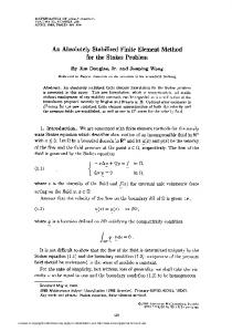
and thus will mix the usage of three words: grid, triangulation, and mesh. We also identify the words ‘node’ and ‘vertex’ since only linear element will be used in this paper. There are two conditions that we shall impose on triangulations that are important in the finite element computation. The first requirement is a topological property. A triangulation T is called conforming or compatible if the intersection of any two simplexes τ and τ 0 in T is either empty or a common lower dimensional simplex (nodes in two dimensions, nodes and edges in three dimensions). The node falls into the interior of a simplex is called a hanging node; See Figure 1 (a).

(a) Bisectwith a triangle (a)a hanging Bisect a triangle (a) A triangulation node

(b) Completion (b) Completion (b) A conforming triangulation

F IGURE 1.F IGURE Newest vertex Newest bisection vertex bisection F IGURE 1. Two triangulations. The left 1. is non-conforming and the right is conforming.

The second important condition is on the geometric structure. A set of triangulations T is called shape regular if there exists a constant c0 such that (4)

max τ ∈T

diam(τ )d ≤ c0 , |τ |

∀T ∈ T ,

where diam(τ ) is the diameter of τ . In two dimensions, it is equivalent to the minimal angle of each triangulation is bounded below uniformly in the shape regular class. Remark 3.2. In addition to (4), if there exists a constant c1 such that maxτ ∈T |τ | (5) ≤ c1 , ∀ T ∈ T , minτ ∈T |τ | T is called quasi-uniform. 3.2. Abstract simplex and simplicial complex. To distinguish the topological structure with geometric one, we now understand the points as abstract entities and introduce abstract simplex or combinatorial simplex [48]. The set τ = {v1 , · · · , vd+1 } of d + 1 abstract points is called an abstract d-simplex. A face σ of a simplex τ is a simplex determined by a non-empty subset of τ . A proper face is any face different from τ . Let N = {v1 , v2 , · · · , vN } be a set of N abstract points. An abstract/combinatorial simplicial complex T is a set of simplices formed by finite subsets of N such that (1) if τ ∈ T is a simplex, then any face of τ is also a simplex in T ; (2) for two simplices τ1 , τ2 ∈ T , the intersection τ1 ∩ τ2 is a face of both τ1 and τ2 . By the definition, a two dimensional combinatorial simplicial complex T contains not only triangles but also edges and vertices of these triangles. A geometric triangulation defined before is only a set of d-simplex but no faces. By including all faces, we shall get a simplicial complex if the triangulation is conforming which corresponds to the second requirement of a simplicial simplex. A subset M ⊂ T is a subcomplex of T if M is a simplicial complex itself. Important classes of subcomplex includes the star or ring of a simplex. That is for a simplex σ ∈ T star(σ) = {τ ∈ T , σ ⊂ τ }. If two, or more, simplices of T share a common face, they are called adjacent or neighbors. The boundary of T is formed by any proper face that belongs to only one simplex, and its faces.

1

1

iFEM

7

By associating the set of abstract points with geometric points in Rn , n ≥ d, we obtain a geometric shape consisting of piecewise flat simplices. This is called a geometric realization of an abstract simplicial complex or, using the terminology of geometry, the embedding of T into Rn . The embedding is uniquely determined by the identification of abstract and geometric vertices. A planar triangulation is a two dimensional abstract simplicial complex which can be embedded into R2 and thus called 2-D triangulation. A 2-D simplicial complex could also be embedding into R3 and result a triangulation of a surface. Therefore the surface mesh in R3 is usually called 2 12 -D triangulation. For these two different embedding, they many have the same combinatorary structure as an abstract simplicial complex but different geometric structure by representing a flat domain in R2 or a surface in R3 . 3.3. Data structure for triangulations. We shall discuss the data structure to represent triangulations and facilitate the mesh adaptation procedure. There is a dilemma for the data structure in the implementation level. If more sophisticated data structure is used to easily traverse in the mesh, for example, to save the star of vertices or edges, it will simplify the implementation of most adaptive finite element subroutines. On the other hand, if the triangulation is changed, for example, a triangle is bisected, one has to update those data structure which in turn complicates the implementation. Our solution is to maintain two basic data structure and construct auxiliary data structure inside each subroutine when it is necessary. It is not optimal in terms of the computational cost. But it will benefit the interface of accessing subroutines, simplify the coding and save the memory. Also as we shall see soon, the auxiliary data structure can be constructed by sparse matrixlization efficiently. This is an example we scarifies a small factor of efficiency to gain the simplicity. 3.3.1. Basic data structure. The matrices node(1:N,1:d) and elem(1:NT,1:d+1) are used to represent a d-dimensional triangulation embedded in Rd , where N is the number of vertices and N T is the number of elements. These two matrices represent two different structure of a triangulation: elem for the topology and node for the embedding. The matrix elem represents a set of abstract simplices. The index set {1, 2, · · · , N } is called the global index set of vertices. Here a vertex is thought as an abstract entity. By definition, elem(t,1:d+1) are the global indices of d + 1 vertices which form the abstract d-simplex t. Note that any permutation of vertices of t will represent the same abstract simplex. The matrix node gives the geometric realization of the simplicial complex. For example, for a 2-D triangulation, node(k,1:2) contain x- and y-coordinates of the k-th node. We shall always order the vertices of a simplex such that the signed volume is positive. That is in 2-D, three vertices of a triangle is ordered counter-clockwise and in 3-D, the ordering of vertices follows the right-hand rule. Note that even permutation of vertices is still allowed to represent the same element. As an example, node and elem matrices to represent the triangulation of the L-shape domain (−1, 1) × (−1, 1)\([0, 1] × [0, −1]) in the Figure 2 (a) and (b). 3.3.2. Auxiliary data structure for 2-D triangulation. We shall discuss how to extract the topological or combinatorial structure of a triangulation by using elem array only. The combinatorial structure will benefit the implementation of finite element methods. edge. We first complete the 2-D simplicial complex by constructing the 1-dimensional simplex. In the matrix edge(1:NE,1:2), the first and second rows contain indices of the starting and ending points. The column is sorted in the way that for the k-th edge, edge(k,1)theta*max(eta))=1; case ’COARSEN’ isMark(etamaxN), break; end

% REFINE

end

We compute the H 1 and L2 norm of the error u − uh using 1-point and 3-points (in 2-D) or 4-points (in 3-D) quadrature rules, respectively. Figure 8 and Figure 9 evidently show our mesh adaptation achieves the optimal convergent order. H1 error and L2 error −1

10

−2

10

−3

10

−4

10

||Du−Duh|| N−0.5 ||u−uh|| N−1

−5

10

3

4

10

10

5

10

F IGURE 8. Convergent rate of 2-D crack problem.

H1 error and L2 error

−1

10

−2

10

||Du−Duh||

−3

10

N−1/3 ||u−uh|| N−2/3

3

10

4

10

5

10

F IGURE 9. Convergent rate of 3-D Cube problem To show our package can handle large size computation, we list the computational cost in Table 3 and Table 4. The time is measured in seconds. The simulation is done using MATLAB 7.6 in a MacBook Pro laptop with configuration: 2.16 GHz Intel Core 2 Duo and 2 GB 667 MHz DDR2 SDRAM. In short, in a standard laptop, our code can simulate a 2-D problem with size 105 in 3 seconds and a 3-D problem in 8 seconds.

32

LONG CHEN

Table 4 shows that the complexity for the 3-D cube problem is indeed linear for small size of unknowns but when the number of unknowns is big, it increases faster than linear rate. In contrast, Table 3 shows that up the scale of 105 , the complexity for the 2-D problem behaves linear with respect to the number unknowns. Detailed profile shows that the solver part takes more than 50% CPU time when the size becomes large. Indeed the director solver build in MATLAB is not of linear complexity. Since the stiffness matrix in 3-D is more dense than that in 2-D, the solver issue is more serious for 3-D problems. We shall address this issue by using multigrid elsewhere. Also the 3-D refinement subroutine is 2 times slower than the counterpart in 2-D. NT Time

NT Time

6534 8839 11990 15842 21140 27903 36959 48846 63940 84038 110598 0.11 0.13 0.19 0.25 0.53 0.61 0.74 1.01 1.29 1.74 2.25 TABLE 3. Computational cost of 2-D crack problem. The first row is the number of elements in each loop and the second row is the CPU time for each loop. The time is measured in second.

1296 2208 3168 4848 8320 12614 19872 31584 49488 74400 119088 0.15 0.21 0.30 0.36 0.60 0.76 1.06 1.72 2.90 5.21 7.98 TABLE 4. Computational cost of 3-D cube problem. The first row is the number of elements in each loop and the second row is the CPU time for each loop. The time is measured in second.

8. C ONCLUSION AND FUTURE WORK In this paper, we have introduced a novel programming style, sparse matrixlization, and developed an efficient MATLAB package, iFEM, for the adaptive finite element methods. Our package can let researchers considerably reduce development time than traditional programming methods. The package can be downloaded from the website http://ifem.wordpress.com. We should be cautious on the sparse matrixlization of the code. Writing efficient matrixlization code requires a higher level of abstraction and a different way of thinking: Think in Matrix. The code is often less readable and thus affect the easy access of package and understanding of the algorithm. It is not worth to spend two hours to optimize the code while only marginal saving on the running time, say one second over total one minute, is achieved [1]. Contrast to many existing MATLAB packages on finite element methods, iFEM can solve middle size problems in few seconds. Since our package heavily relies on the sparse matrix package, we could further improve the performance of iFEM by combining other sparse matrix packages. We should also mention the limitation of our package. Only linear element and fixed quadrature rule is implemented. The code is still one magnitude slower than packages written by Fortran or C such as ALBERTA [56], MC [31], PHG [63], and PLTMG [7]. Therefore researchers should be aware on the trade-off between the considerably shorter development time and the slightly lower performance. The data structure introduced in this paper can be used to implement other methods such as quadratic finite element, mixed finite element methods, non-conforming finite element methods, and edge element for electromangnetics. These elements will be added into our package in a near future. A h-p adaptive finite element package is also possible, but requiring further design of data structure. One nice benefit of sparse matrixlization is the potential scaling characteristics of codes implemented in iFEM. Except the codes involving sparse matrix operations, other parts, e.g., the bisection of marked

iFEM

33

elements, are embarrassingly parallel (the tasks really or never communicate). Provided the parallelization of sparse matrix package, the bisection and coarsening can then be easily parallelized, which in contrast may not be easy for code writing in traditional (sequential) styles. We mention that a parallelization of newest vertex bisection can be found in [41] for 2-D and in [63] for 3-D. It is worth noting that 3-D coarsening is not discussed in this paper. Our decomposition of bisection grids presented in Section 6 holds for bisection methods in any dimensions. But the characterization of compatible star in three dimensions is missing. To do so, we need newest vertex type bisection not longest edge bisection. Additional data structure like the type of elements should be introduced to reduce the combinatory complication. This will be studied and reported elsewhere. We also note that the computational cost is not scaled linearly with respect to the size of the problem. This is due to the direct solver in MATLAB which is not of optimal (linear) complexity. We have implemented 2-D multigrid based on our coarsening algorithm which is of optimal complexity. Efficient 3-D multigrid will be implemented when coarsening in 3-D is available or by introducing additional data structure. This will be also studied and reported elsewhere. Historical remark. The author has written a short package [15] of AFEM for elliptic partial differential equations in early 2006 and successfully used it to teach graduate students in 2006 summer school at the Peking University. In late 2006, Chensong Zhang and the author improved it into a more completed package for two dimensional elliptic problems: AFEM@matlab [17], which has already been used in several recent publications [17, 62, 32]. iFEM is different with AFEM@matlab in several aspects: the data structure is updated and constructed more efficiently, the main subroutines are rewritten using new data structure and sparse matrixlization to improve the efficiency. More importantly, three dimensional adaptive finite element method is included. Acknowledgement. The author would like to thank Professor Michael Holst in University of California at San Diego for the discussion on the data structure for three dimensional mesh refinement and finite element computation, Professor Ludmil Zikatanov in Pennsylvania State University for the discussion on the usage of sparse matrix in the data structure, and also Dr. Chensong Zhang in Pennsylvania State University for the effort in the development of AFEM@matlab, the early version of iFEM. R EFERENCES [1] P. J. Acklam. MATLAB array manipulation tips and tricks. Notes, 2003. [2] J. Alberty, C. Carstensen, and S. A. Funken. Remarks around 50 lines of Matlab: short finite element implementation. Numerical Algorithms, 20:117–137, 1999. [3] J. Alberty, C. Carstensen, S. A. Funken, and R. Klose. Matlab implementation of the finite element method in elasticity. Computing, 69(3):239–263, 2002. [4] D. N. Arnold, A. Mukherjee, and L. Pouly. Locally adapted tetrahedral meshes using bisection. SIAM Journal of Scientific Computing, 22(2):431–448, 2000. [5] I. Babuˇska and M. Vogelius. Feeback and adaptive finite element solution of one-dimensional boundary value problems. Numerische Mathematik, 44:75–102, 1984. [6] C. Bahriawati and C. Carstensen. Three matlab implementations of the lowest-order Raviart-Thomas MFEM with a posteriori error control. Computational Methods In Applied Mathematics, 5(4):333–361, 2005. [7] R. E. Bank. PLTMG: A software package for solving elliptic partial differential equations users’ guide 9.0. Department of Mathematics, University of California at San Diego, 2004. [8] R. E. Bank, A. H. Sherman, and A. Weiser. Refinement algorithms and data structures for regular local mesh refinement. In Scientific Computing, pages 3–17. IMACS/North-Holland Publishing Company, Amsterdam, 1983. [9] E. B¨ansch. Local mesh refinement in 2 and 3 dimensions. Impact of Computing in Science and Engineering, 3:181–191, 1991. [10] S. Bartels, C. Carstensen, and A. Hecht. P2q2iso2d=2d isoparametric fem in matlab. Journal of Computational and Applied Mathematics, 192(2):219–250, 2006. [11] J. Bey. Tetrahedral grid refinement. Computing, 55(4):355–378, 1995. [12] T. C. Biedl, P. Bose, E. D. Demaine, and A. Lubiw. Efficient algorithms for Petersen’s matching theorem. In Symposium on Discrete Algorithms, pages 130–139, 1999.

34

LONG CHEN

[13] S. C. Brenner and L. R. Scott. The mathematical theory of finite element methods, volume 15 of Texts in Applied Mathematics. Springer-Verlag, New York, second edition, 2002. [14] C. Carstensen and R. Klose. Elastoviscoplastic finite element analysis in 100 lines of Matlab. J. Numer. Math., 10(3):157– 192, 2002. [15] L. Chen. Short implementation of bisection in MATLAB. In P. Jorgensen, X. Shen, C.-W. Shu, and N. Yan, editors, Recent Advances in Computational Sciences – Selected Papers from the International Workship on Computational Sciences and Its Education, pages 318 – 332, 2008. [16] L. Chen, R. H. Nochetto, and J. Xu. Multilevel methods on graded bisection grids I: H 1 system. Preprint, 2007. [17] L. Chen and C.-S. Zhang. AFEM@matlab: a Matlab package of adaptive finite element methods. Technique Report, Department of Mathematics, University of Maryland at College Park, 2006. [18] L. Chen and C.-S. Zhang. A coarsening algorithm and multilevel methods on adaptive grids by newest vertex bisection. Technique Report, Department of Mathematics, University of Maryland at College Park, 2007. [19] J. Chessa. Programing the finite element method with matlab. 2002. [20] P. G. Ciarlet. The Finite Element Method for Elliptic Problems, volume 4 of Studies in Mathematics and its Applications. North-Holland Publishing Co., Amsterdam-New York-Oxford, 1978. [21] M. Dabrowski, M. Krotkiewski, and D. Schmid. MILAMIN: MATLAB-based finite element method solver for large problems. Geochemistry Geophysics Geosystems, 9(4), 2008. [22] T. Davis. Creating sparse Finite-Element matrices in MATLAB. http://blogs.mathworks.com/loren/2007/03/01/creatingsparse-finite-element-matrices-in-matlab/, 2007. [23] T. A. Davis. Direct methods for sparse linear systems, volume 2 of Fundamentals of Algorithms. Society for Industrial and Applied Mathematics (SIAM), Philadelphia, PA, 2006. [24] W. D¨orfler. A convergent adaptive algorithm for Poisson’s equation. SIAM Journal on Numerical Analysis, 33:1106–1124, 1996. [25] I. S. Duff, A. M. Erisman, and J. K. Reid. Direct methods for sparse matrices. Monographs on Numerical Analysis. The Clarendon Press Oxford University Press, New York, second edition, 1989. Oxford Science Publications. [26] H. C. Elman, A. Ramage, and D. J. Silvester. Algorithm 866: IFISS, a Matlab toolbox for modelling incompressible flow. ACM Transactions on Mathematical Software, 33(2):14, June 2007. Article 14, 18 pages. [27] H. C. Elman, A. Ramage, and D. J. Silvester. Algorithm 866: Ifiss, a matlab toolbox for modelling incompressible flow. ACM Trans. Math. Softw., 33(2):14, 2007. [28] S. Funken, D. Praetorius, and P. Wissgott. Efficient implementation of adaptive P1-FEM in MATLAB. Preprint, 2008. [29] J. R. Gilbert, C. Moler, and R. Schreiber. Sparse matrices in MATLAB: design and implementation. SIAM J. Matrix Anal. Appl., 13(1):333–356, 1992. [30] M. Holst. MCLite: An adaptive multilevel finite element MATLAB package for scalar nonlinear elliptic equations in the plane. UCSD Technical report and guide to the MCLite software package, 2000. [31] M. Holst. Adaptive numerical treatment of elliptic systems on manifolds. Advances in Computational Mathematics, 15:139– 191, 2001. [32] R. H. W. Hoppe, G. Kanschat, and T. Warburton. Convergence analysis of an adaptive interior penalty discontinuous galerkin method. Technical report, Texas A & M University, 2007. [33] I. Kossaczk´ y . A recursive approach to local mesh refinement in two and three dimensions. Journal of Computational and Applied Mathematics, 55:275–288, 1994. [34] Y. W. Kwon and H. Bang. The finite element method using MATLAB. CRC Mechanical Engineering Series. Chapman & Hall/CRC, Boca Raton, FL, second edition, 2000. With 1 CD-ROM (Windows 95, 98 or NT4.0). [35] J. Li and Y.-T. Chen. Computational Partial Differential Equations Using MATLAB. Applied Mathematics & Nonlinear Science. Chapman & Hall/CRC, 2008. [36] A. Liu and B. Joe. Quality local refinement of tetrahedral meshes based on bisection. SIAM Journal on Scientific Computing, 16(6):1269–1291, 1995. [37] J. Maubach. Local bisection refinement for n-simplicial grids generated by reflection. SIAM Journal of Scientific Computing, 16(1):210–227, 1995. [38] W. F. Mitchell. Unified Multilevel Adaptive Finite Element Methods for Elliptic Problems. PhD thesis, University of Illinois at Urbana-Champaign, 1988. [39] W. F. Mitchell. A comparison of adaptive refinement techniques for elliptic problems. ACM Transactions on Mathematical Software (TOMS) archive, 15(4):326 – 347, 1989. [40] W. F. Mitchell. Optimal multilevel iterative methods for adaptive grids. SIAM Journal on Scientific and Statistical Computing, 13:146–167, 1992. [41] W. F. Mitchell. A refinement-tree based partitioning method for dynamic load balancing with adaptively refined grids. Journal of Parallel and Distributed Computing, 67(4):417–429, 2007. [42] P. Morin, R. H. Nochetto, and K. G. Siebert. Convergence of adaptive finite element methods. SIAM Review, 44(4):631–658, 2002. [43] P.-O. Persson and G. Strang. A simple mesh generator in matlab. SIAM Review, 46(2):329–345, 2004.

iFEM

35

[44] S. Pissanetsky. Sparse matrix technology. Academic Press, 1984. [45] A. Plaza and G. F. Carey. Local refinement of simplicial grids based on the skeleton. Applied Numerical Mathematics, 32(2):195–218, 2000. [46] A. Plaza, M. A. Padron, and G. F. Carey. A 3d refinement/derefinement algorithm for solving evolution problems. Applied Numerical Mathematics, 32(4):401–418, 2000. [47] A. Plaza and M.-C. Rivara. Mesh refinement based on the 8-tetrahedra longest-edge partition. 12th meshing roundtable, 2003. [48] K. Polthier. Computational aspects of discrete minimal surfaces. In Global theory of minimal surfaces, volume 2 of Clay Math. Proc., pages 65–111. Amer. Math. Soc., Providence, RI, 2005. [49] C. Pozrikidis. Introduction To Finite And Spectral Element Methods Using Matlab. Chapman & Hall/CRC, 2005. [50] M. C. Rivara. Mesh refinement processes based on the generalized bisection of simplices. SIAM Journal on Numerical Analysis, 21:604–613, 1984. [51] M.-C. Rivara and P. Inostroza. Using longest-side bisection techniques for the automatic refinement fo Delaunay triangulations. International Journal for Numerical Methods in Engineering, 40:581–597, 1997. [52] M. C. Rivara and G. Iribarren. The 4-triangles longest-side partition of triangles and linear refinement algorithms. Mathemathics of Computation, 65(216):1485–1501, 1996. [53] M. C. Rivara and M. Venere. Cost analysis of the longest-side (triangle bisection) refinement algorithms for triangulations. Engineering with Computers, 12:224–234, 1996. [54] Y. Saad. Iterative methods for sparse linear systems. Society for Industrial and Applied Mathematics, Philadelphia, PA, second edition, 2003. [55] A. Schmidt and K. G. Siebert. Design of adaptive finite element software, volume 42 of Lecture Notes in Computational Science and Engineering. Springer-Verlag, Berlin, 2005. The finite element toolbox ALBERTA, With 1 CD-ROM (Unix/Linux). [56] A. Schmidt and K. G. Siebert. The finite element toolbox ALBERTA. Springer-Verlag, Berlin, 2005. [57] E. G. Sewell. Automatic generation of triangulations for piecewise polynomial approximation. In Ph. D. dissertation. Purdue Univ., West Lafayette, Ind., 1972. [58] R. Stevenson. The completion of locally refined simplicial partitions created by bisection. Mathemathics of Computation, 77:227–241, 2008. [59] C. T. Traxler. An algorithm for adaptive mesh refinement in n dimensions. Computing, 59(2):115–137, 1997. [60] L. N. Trefethen. Spectral methods in MATLAB, volume 10 of Software, Environments, and Tools. Society for Industrial and Applied Mathematics (SIAM), Philadelphia, PA, 2000. [61] L. N. Trefethen. Ten digit algorithms. Mitchell Lecture, June 2005. [62] J. Xu, Y. Zhu, and Q. Zou. Convergence analysis of adaptive finite volume element methods for general elliptic equations. (submitted), 2006. [63] L. Zhang. A parallel algorithm for adaptive local refinement of tetrahedral meshes using bisection. NUMERICAL MATHEMATICS: Theory, Methods and Applications, 2008. D EPARTMENT OF M ATHEMATICS , U NIVERSITY OF C ALIFORNIA AT I RVINE , I RVINE , CA 92697 E-mail address: [email protected]