TECHNO BYTES
Image distortion and spatial resolution of a commercially available cone-beam computed tomography machine John W. Ballrick,a J. Martin Palomo,b Edward Ruch,c B. Douglas Amberman,d and Mark G. Hanse Cleveland, Ohio Introduction: Our objective was to evaluate images produced by a commercially available cone-beam computed tomography (CBCT) machine (i-CAT model 9140-0035-000C, Imaging Sciences International, Hatfield, Pa) for measurement and spatial resolution (ie, the ability to separate 2 objects in close proximity in the image) for all settings and in all dimensions. Methods: A custom phantom containing 0.3 mm diameter chromium metal markers approximately 5 mm apart in 3 planes of space was developed for analyzing distortion and measurement accuracy. This phantom was scanned in the CBCT machine by using all 12 commercially available settings. The distance between the markers was measured 3 times on the 3-dimensional images by using a Digital Imaging and Communications in Medicine (DICOM) viewer and was also measured 3 times directly on the phantom with a fine-tipped digital caliper. A line-pair phantom was used to evaluate spatial resolution. Thirty evaluators analyzed images and assigned a resolution from 0.2 to 1.6 mm according to the separation of the line pairs. Results: There were no statistically significant differences among the 3-dimensional images for any setting, in any dimension, or in images divided by thirds in terms of measurement accuracy. Comparison of the CBCT measurements to the direct digital caliper measurements showed a statistically significant difference (P ⬍0.01). However, the absolute difference was ⬍0.1 mm and is probably not clinically significant for most applications. The worst spatial resolution found was 0.86 mm. Spatial resolution was lower at faster scan times and larger voxel sizes. Conclusions: This CBCT machine has clinically accurate measurements and acceptable resolution. (Am J Orthod Dentofacial Orthop 2008;134:573-82)
C
one-beam computed tomography (CBCT) is a burgeoning technology with the ability to change how orthodontists look at their patients. CBCT can show 3-dimensional (3D) structures in 3 dimensions. In years past, this has been practical and cost effective only with study models. In dental imaging, CBCT is making inroads in many dental offices and dental imaging centers as a more complete method for diagnosis and treatment planning in true 3 dimensions and a 1:1 perspective, rather than with enlarged or distorted images. A recent article stated that the techFrom the School of Dental Medicine, Case Western Reserve University, Cleveland, Ohio. a Former resident, Department of Orthodontics; private practice, Rocky River and Westlake, Ohio. b Associate professor, Department of Orthodontics. c Clinical associate professor, Departments of Oral Diagnosis and Radiology and Oral Maxillofacial Surgery. d Professor, Department of Orthodontics. e Professor and chairman, Department of Orthodontics. Reprint requests to: J. Martin Palomo, Case Western Reserve University, School of Dental Medicine, Department of Orthodontics, 10900 Euclid Ave, Cleveland, OH 44106; e-mail,
[email protected]. Submitted, October 2007; revised and accepted, November 2007. 0889-5406/$34.00 Copyright © 2008 by the American Association of Orthodontists. doi:10.1016/j.ajodo.2007.11.025
nology is “initiating a trend in which traditional orthodontic imaging is being replaced by 3D imaging.”1 The advantages of this technology are fairly low cost and convenient size compared with traditional computed tomography machines, 3D images of dentofacial regions, ease of operation, relatively quick scans, low radiation exposure, and the elimination of many x-rays to localize anatomic structures.2 CBCT technology is able to achieve radiation dose levels equivalent to a full-mouth series, and as low as 2 panoramic radiographs, depending on the setting in use.3-5 The settings (mA, kVp, exposure time, etc) being used determines the radiation dose, and directly influence image quality.4 In spite of this slight increase in radiation, all necessary radiographs can be collected in 1 scan in less than a minute. In addition, views not previously available can be created—axial, coronal, sagittal, and separate views of the right and left sides of the head.6 The uses of these images include dental implant planning, temporomandibular joint imaging, locating the mandibular nerve canal, studying mixed dentitions, planning temporary orthodontic anchorage devices, identifying and locating pathologic lesions, evaluating endodontic problems, locating supernumerary teeth, evaluating al573
574 Ballrick et al
American Journal of Orthodontics and Dentofacial Orthopedics October 2008
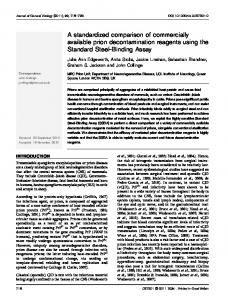
Fig 1. The CIC phantom viewed at different angles and 0.3-mm chromium spheres compared with a ruler.
veolar ridge height and volume, evaluating growth and development of the craniofacial complex, analyzing the airway, and studying the development of surgical guides and stents.7 One article has gone so far as to suggest that “this new technology has become the standard of care in diagnosing and treating dental pathology, abnormalities/problems in craniofacial growth and development, and in performing analysis for mixed dentitions, as well as for dental implants.”8 Dental radiographs and photographs are commonly used in the diagnosis and treatment planning of patients in orthodontics. These 2-dimensional images are subject to geometric, rotational, and head-positioning errors that can cause the area of interest to be misrepresented.9 Many clinicians have searched for 3D representations of anatomic structures without these problems. The development of 3D modeling of patient anatomy would help to determine appropriate treatment options, monitor changes, detect treatment results, and measure outcomes more accurately.9 The measurement accuracy of CBCT images has been studied on different machines with varied results. Some authors found no statistically significant differences between CBCT images and anatomic truth,10 whereas others illustrated differences that, even though statistically different, were not considered clinically significant.11-15
The purpose of this study was to determine the measurement accuracy and spatial resolution of a commercially available CBCT dental imaging system with an amorphous flat panel detector. MATERIAL AND METHODS
We used 2 phantoms to determine image size, measurement accuracy, and spatial resolution of a CBCT machine. The phantoms were scanned by using a flat-panel detector CBCT machine (i-CAT model 9140-0035-000C, Imaging Sciences International, Hatfield, Pa) at a commercial dental imaging center (Toothpics Dental Imaging Center, Beachwood, Ohio). The study consisted of 2 parts: an evaluation of measurement accuracy and an evaluation of spatial resolution. The first phantom (craniofacial imaging center [CIC] phantom) was custom made to measure the image size and evaluate measurement accuracy (Fig 1). The CIC phantom is acrylic with embedded chromium spheres (Small Parts, Miami Lakes, Fla). The spheres are 0.3 mm in diameter and are placed approximately every 5 mm in a row. There are 3 such rows with 1 in each of the x, y, and z planes having a common central point of intersection. The radiographic settings of the CBCT machine are preset and fixed (Table I). Data were collected by using the 12 commercially available settings. The phantom
Ballrick et al 575
American Journal of Orthodontics and Dentofacial Orthopedics Volume 134, Number 4
Table I.
i-CAT image setting information
Requested size (cm)
Height
Width
Depth
Scan time (s)*
Voxel size (mm)*
Exposure (s)*
mAs*
Raw images
Primary reconstruction axial slices
13 13 13 13 13 8 6 mandibular 6 maxillary 6 6 6 mandibular 6 maxillary
12.81 12.82 12.82 12.82 12.82 7.88 5.45 5.44 5.46 5.44 5.47 5.48
16.02 15.99 16.02 16.03 16.06 16.03 16.05 16.00 16.03 16.05 16.03 16.04
16.01 16.00 16.03 16.05 16.05 16.05 16.00 16.02 16.04 16.02 16.02 16.04
40 20 10 20 40 20 20 20 10 10 40 40
0.4 0.4 0.4 0.3 0.25 0.4 0.4 0.4 0.4 0.3 0.2 0.2
7.2 3.6 1.8 3.6 7.2 3.6 3.6 3.6 1.8 1.8 7.2 7.2
47 24 12 24 47 24 24 24 12 12 47 47
599 306 160 306 599 306 599 599 160 160 306 306
323 323 323 430 516 200 138 138 138 183 277 277
Actual size (cm)
All images collected at 120 kVp and 5 mA. *Manufacturer’s specifications.
Fig 2. Full view of the C phantom and a close up view from the top showing the 9 series of metal lines used to assess image resolution.
was placed in the machine in a reproducible method, with the center of the phantom in the center of the scout image. The raw data were collected from the machine, and software (i-CAT software, version 2.2.21) was used to reconstruct the raw data. Once the reconstruction was completed, the information was exported as a Digital Imaging and Communications in Medicine (DICOM) file. The data were then imported, analyzed, and measured with Accurex (version 1.1, Cybermed, Seoul, South Korea). The digital images were evaluated by using the sagittal slices for height and the axial slices for width and depth. The center-to-center distances of the metal spheres were measured directly on the CIC phantom with a
fine-point digital caliper accurate to 0.01 mm resolution (500 series, Mitutoyo America, Aurora, Ill). Manual measurements were collected and compared with the digital measurements in the software. All measurements, direct and on the computer, were made at 3 separate times. The mean of the 3 times was used to minimize possible measurement errors. The second phantom, called the C phantom (Phantom Laboratory, Salem, NY), is a high-contrast line-pair phantom (used to evaluate an image’s spatial resolution (Fig 2). The C phantom is made of acrylic and metal plates that are submerged in distilled water. The phantom contains 9 series of 4 plates placed parallel at decreasing distances apart. The image resolution is established by determining
576 Ballrick et al
at which series of plates there is a clear distinction between each plate. The range of resolution that can be tested with this phantom is 0.35 to 1 mm. The image resolution was collected by determining the separation of the lines from the C phantom in sagittal slice images for the 12 available settings of the CBCT machine. All images were standardized for brightness and contrast and were magnified to the same extent. Thirty volunteers were used to evaluate the collected images. PowerPoint (Microsoft, Redmond, Wash) was used to present the images in a standardized format on a 21-in liquid-crystal-display flat-panel monitor (Dell Computer, Round Rock, Tex) in a dim room. The evaluators were first asked to determine the choices that showed a clear, distinct separation of the 4 lines of the line-pair phantom, which is the manufacturer’s recommendation for interpretation. In addition, the evaluators were asked to determine the choices that allowed identification of a pattern of 4 lines, although the lines might not have had clear delineation. To determine the reliability of the answers, 24 slides were shown with 2 separate slides for each image setting. The average resolution for each image setting was calculated by averaging both readings for each method of evaluation. The images were ranked based on the average resolution. A ranking of 1 represented the best spatial resolution, and 12 was the worst spatial resolution. This method of spatial resolution evaluation was similar to a previously described method.16 Statistical analysis
The data collected were continuous and appropriately organized by using Excel 2007 spreadsheets (Microsoft). Excel 2007 was used for descriptive statistics, and SPSS software (version 14, SPSS, Chicago, Ill) was used for further analysis. To assess measurement accuracy, the absolute mathematical differences were used to describe differences between the Accurex software measurements and the direct digital caliper measurements. The same procedure was also used, with the images further divided into thirds for each dimension. The mean absolute differences for the 12 image settings in all dimensions were normally distributed; therefore, analysis of variance (ANOVA) at P ⫽ 0.05 was used to determine whether there were any significant differences between the settings or the dimensions. Further analysis pooled all measurements for all settings, dimensions, and thirds. After determining that the data were normally distributed, we directly compared the measurements from the CBCT with the same measurements made with the digital caliper using a pairedsample t test at P ⫽ 0.05. Measurement differences of
American Journal of Orthodontics and Dentofacial Orthopedics October 2008
less than 0.1 mm were considered clinically insignificant. To determine how the various image settings affected the observed resolution values, a multiple regression was used. The dependent variable was the image resolution value, and the independent variables were image size, seconds of scan, and voxel size. The coefficient of determination (R2) was calculated for each image parameter and for the combination of the 2 most influential parameters. For reliability of the measurements, the measures for the scans of the CIC phantom were repeated several times. An intraclass correlation coefficient (ICC) was used to assess measurements at different times to assess intraoperator reliability. In addition, the standard deviations were established for each measurement, and the overall standard deviation for each image setting and dimension was determined. A calculation of ⫾ 2 SD showed the range of where 95% of measurements would be expected to fall. For the reliability of the C phantom images, each image was presented twice to assess intraexaminer reliability. Reliability was calculated by using an ICC. RESULTS
Measurements from the CBCT and the digital caliper showed excellent intraoperator reliability, with ICC values of 0.892 for the CBCT measurements and 0.902 for the direct digital caliper measurements. The reliability for measurement accuracy using the standard deviations of the measurements for the 12 image settings measured by the CBCT and directly with digital caliper ranged from 0.017 to 0.072 mm. This indicated that 95% of all measurements were within a maximum of ⫾ 0.144 mm (Table II). The 30 evaluators for the evaluation of the C phantom showed excellent reliability. This reliability was demonstrated in both methods of evaluation but was higher when the evaluators were asked to identify a pattern of 4 lines, although the lines might not have had clear delineation (ICC values of 0.78 for clear separation of lines and 0.91 for identification of a pattern of lines). ANOVA for the mean absolute differences between the CBCT measurements and the direct digital caliper measurements indicated no statistically significant differences (P ⫽ 0.964) between any image settings or dimensions (Table III). There was a general trend of the CBCT measurements to be smaller than the direct digital caliper measurements in 94.4% of the measurements (Table III). Further subdivision of the dimensions into thirds also showed no statistically significant differences (P ⫽ 0.259) between any image settings or
Ballrick et al 577
American Journal of Orthodontics and Dentofacial Orthopedics Volume 134, Number 4
Table II.
Intraoperator measurement reliability by standard deviations Height
Image setting 13 cm, 40 s, 0.4 mm voxel 13 cm, 20 s, 0.4 mm voxel 13 cm, 10 s, 0.4 mm voxel 13 cm, 20 s, 0.3 mm voxel 13 cm, 40 s, 0.25 mm voxel 8 cm, 20 s, 0.4 mm voxel 6 cm, 20 s, 0.4 mm voxel, mandibular 6 cm, 20 s, 0.4 mm voxel, maxillary 6 cm, 10 s, 0.4 mm voxel 6 cm, 10 s, 0.3 mm voxel 6 cm, 40 s, 0.2 mm voxel, mandibular 6 cm, 40 s, 0.2 mm voxel, maxillary Direct measurement
Table III.
Width
Depth
SD average (mm)
95% of measures
SD average (mm)
95% of measures
SD average (mm)
95% of measures
0.052 0.052 0.047 0.036 0.047 0.042 0.033 0.040 0.029 0.037 0.017 0.025 0.047
⫾ 0.104 ⫾ 0.104 ⫾ 0.094 ⫾ 0.072 ⫾ 0.094 ⫾ 0.084 ⫾ 0.066 ⫾ 0.080 ⫾ 0.058 ⫾ 0.074 ⫾ 0.034 ⫾ 0.050 ⫾ 0.094
0.065 0.061 0.048 0.052 0.051 0.060 0.046 0.032 0.038 0.038 0.041 0.041 0.044
⫾ 0.130 ⫾ 0.122 ⫾ 0.096 ⫾ 0.104 ⫾ 0.102 ⫾ 0.120 ⫾ 0.092 ⫾ 0.064 ⫾ 0.076 ⫾ 0.076 ⫾ 0.082 ⫾ 0.082 ⫾ 0.088
0.072 0.057 0.055 0.045 0.056 0.059 0.039 0.046 0.057 0.051 0.043 0.040 0.042
⫾ 0.144 ⫾ 0.114 ⫾ 0.110 ⫾ 0.090 ⫾ 0.112 ⫾ 0.118 ⫾ 0.078 ⫾ 0.092 ⫾ 0.114 ⫾ 0.102 ⫾ 0.086 ⫾ 0.080 ⫾ 0.084
Mean absolute differences between CBCT measurements and direct measurements of the CIC phantom Height
Image setting 13 cm, 40 s, 0.4 mm voxel 13 cm, 20 s, 0.4 mm voxel 13 cm, 10 s, 0.4 mm voxel 13 cm, 20 s, 0.3 mm voxel 13 cm, 40 s, 0.25 mm voxel 8 cm, 20 s, 0.4 mm voxel 6 cm, 20 s, 0.4 mm voxel, mandibular 6 cm, 20 s, 0.4 mm voxel, maxillary 6 cm, 10 s, 0.4 mm voxel 6 cm, 10 s, 0.3 mm voxel 6 cm, 40 s, 0.2 mm voxel, mandibular 6 cm, 40 s, 0.2 mm voxel, maxillary Mean SD
Width
Depth
Absolute difference (mm)
CBCT minus direct (mm)
Absolute difference (mm)
CBCT minus direct (mm)
Absolute difference (mm)
CBCT minus direct (mm)
0.072 (0.049) 0.056 (0.042) 0.067 (0.053) 0.067 (0.054) 0.060 (0.062) 0.082 (0.063) 0.085 (0.088) 0.071 (0.066) 0.065 (0.065) 0.061 (0.041) 0.058 (0.059) 0.073 (0.063) 0.068 0.009
⫺0.015 (0.087) ⫺0.013 (0.069) ⫺0.020 (0.084) ⫺0.039 (0.077) ⫺0.034 (0.080) ⫺0.020 (0.103) ⫺0.019 (0.124) ⫺0.025 (0.096) 0.008 (0.093) ⫺0.031 (0.070) ⫺0.012 (0.084) ⫺0.036 (0.091) ⫺0.021 0.013
0.074 (0.051) 0.050 (0.042) 0.050 (0.045) 0.046 (0.035) 0.049 (0.037) 0.046 (0.036) 0.047 (0.040) 0.051 (0.040) 0.053 (0.043) 0.055 (0.045) 0.059 (0.040) 0.070 (0.042) 0.054 0.009
⫺0.014 (0.090) ⫺0.005 (0.066) ⫺0.024 (0.063) ⫺0.011 (0.057) 0.007 (0.062) ⫺0.004 (0.058) ⫺0.020 (0.059) ⫺0.029 (0.059) ⫺0.035 (0.059) ⫺0.033 (0.063) ⫺0.046 (0.054) ⫺0.062 (0.054) ⫺0.023 0.019
0.082 (0.066) 0.078 (0.071) 0.064 (0.055) 0.063 (0.048) 0.074 (0.054) 0.071 (0.056) 0.060 (0.052) 0.068 (0.045) 0.063 (0.047) 0.055 (0.047) 0.058 (0.034) 0.061 (0.031) 0.066 0.008
⫺0.059 (0.088) ⫺0.023 (0.104) ⫺0.036 (0.077) ⫺0.044 (0.067) ⫺0.042 (0.082) ⫺0.032 (0.085) ⫺0.029 (0.074) ⫺0.051 (0.064) ⫺0.033 (0.072) ⫺0.024 (0.068) ⫺0.050 (0.046) ⫺0.046 (0.052) ⫺0.039 0.011
P ⫽ 0.964. Means and standard deviations (in parentheses) reported.
thirds of the images (Table IV). A paired-sample t test between the CBCT measurements and the direct digital caliper measurements indicated a statistically significant difference at the P ⬍0.01 level (Table V). The 12 image settings were evaluated by 30 evaluators with no exclusions. The average image resolution for the clear separation of the lines of the line-pair phantom ranged from 0.622 to 0.860 mm; the 6 cm, 40 second, 0.2 mm voxel was the best ranked image, and the 13 cm, 10 second, 0.4 mm voxel was the poorest ranked image. The average image resolution for the identification of a pattern of 4 lines of the line-pair phantom ranged from 0.398 to 0.704 mm; the 6 cm, 40
second, 0.2 mm voxel was the best ranked image, and the 13 cm, 10 second, 0.4 mm voxel was the poorest ranked image. The coefficient of determination (R2) indicated that voxel size had the most effect on resolution; 52.1% of the variation of the clear separation resolutions and 57.8% of the variation of the pattern identification resolutions were explained by voxel size alone. Voxel size was followed by seconds, with 43.9% of clear separation resolution variation and 39.4% of pattern identification resolution variation explained by scan time. Image size had the least effect on resolution, with 22.3% of clear separation resolution variation and 23.2% of pattern identification resolution variation ex-
578 Ballrick et al
American Journal of Orthodontics and Dentofacial Orthopedics October 2008
Table IV.
Mean absolute differences between CBCT measurements and direct measurements of the CIC phantom analyzed by thirds Height
Image setting 13 cm, 40 s, 0.4 mm voxel 13 cm, 20 s, 0.4 mm voxel 13 cm, 10 s, 0.4 mm voxel 13 cm, 20 s, 0.3 mm voxel 13 cm, 40 s, 0.25 mm voxel 8 cm, 20 s, 0.4 mm voxel 6 cm, 20 s, 0.4 mm voxel, mandibular 6 cm, 20 s, 0.4 mm voxel, maxillary 6 cm, 10 s, 0.4 mm voxel 6 cm, 10 s, 0.3 mm voxel 6 cm, 40 s, 0.2 mm voxel, mandibular 6 cm, 40 s, 0.2 mm voxel, maxillary Mean SD
Top
Middle
Bottom
0.037 (0.040) 0.037 (0.039) 0.020 (0.030) 0.028 (0.025) 0.032 (0.036) 0.092 (0.036) 0.112 (0.104) 0.088 (0.088) 0.055 (0.019) 0.068 (0.040) 0.042 (0.043) 0.092 (0.050) 0.059 0.031
0.053 (0.058) 0.087 (0.056) 0.030 (0.056) 0.027 (0.073) 0.015 (0.080) 0.060 (0.084) 0.012 (0.114) 0.028 (0.076) 0.028 (0.093) 0.032 (0.045) 0.033 (0.073) 0.035 (0.081) 0.037 0.021
0.010 (0.044) 0.040 (0.020) 0.060 (0.058) 0.017 (0.041) 0.022 (0.059) 0.052 (0.029) 0.068 (0.038) 0.052 (0.024) 0.035 (0.021) 0.055 (0.044) 0.025 (0.024) 0.018 (0.020) 0.038 0.019
P ⫽ 0.259. Means and standard deviations (in parentheses) reported. Table V.
Paired 2-sample t test for comparing CBCT measurements with direct measurements
Mean (mm) Variance Observations Pearson correlation df t statistic P (T ⱕ t) 2-tail t critical 2-tail
CBCT measurements
Direct measurements
5.12904351 0.026976286 927 0.895953493 926 ⫺12.14551714 1.32926 E –31 1.962529084
5.158349515 0.024288718 927
plained by differences in image size. A combination of voxel size and seconds explained 60.1% of the variation in clear separation resolution and 62.1% of the variation in pattern identification resolution (Table VI). DISCUSSION
The expanding use of CBCT technology is beneficial to both patients and practitioners. A thorough understanding of the theoretical limits of the machines is required to optimize their use. We used phantoms to obtain information about measurement accuracy and image resolution. The CIC phantom and the C phantom had different purposes, but a thorough evaluation of the data illustrates some technical capabilities of this CBCT machine. This information can be used by practitioners to determine ideal settings for a particular circumstance. The CIC phantom was constructed of acrylic with chromium metal markers embedded approximately ev-
ery 5 mm. The metal markers were not always exactly 5 mm apart due to random errors during fabrication. The markers were 0.3 mm in diameter, and this small size made it difficult to precisely position them. Furthermore, when scanned in the CBCT, some metal artifacts were noted. This “halo” effect made some metal markers appear almost 2 times larger than they actually were, and some appeared more elongated than perfectly round. To minimize any effect on measurement of this, the center of the point of maximum density was measured. It is believed that this method minimized errors in the measurement of the images in the software. To fully analyze the accuracy of measurements from the CBCT and the direct digital caliper measurements, it was determined that each measurement between each marker should be made 3 times. This minimized measurement errors and allowed the establishment of means and standard deviations. The mean of the 3 measurements for the CBCT was then compared with the mean of the same measurements from the direct digital caliper. An absolute difference was calculated for these point-to-point measurements, and an average of all absolute differences for the particular dimensions and image settings was calculated. This method might have overlooked areas of variation between points, so the data were further divided into thirds for each dimension to see whether there were any differences between the periphery and the center of the images. ANOVA conducted to test the hypothesis that there were no statistically significant differences between any image settings or dimensions clearly showed
Ballrick et al 579
American Journal of Orthodontics and Dentofacial Orthopedics Volume 134, Number 4
Table IV.
Continued Width
Depth
Left
Middle
Right
Front
Middle
Back
0.072 (0.048) 0.045 (0.049) 0.028 (0.046) 0.040 (0.019) 0.047 (0.032) 0.045 (0.031) 0.068 (0.030) 0.022 (0.030) 0.035 (0.033) 0.040 (0.019) 0.062 (0.030) 0.070 (0.043) 0.048 0.017
0.067 (0.055) 0.027 (0.042) 0.050 (0.048) 0.017 (0.046) 0.067 (0.037) 0.033 (0.046) 0.023 (0.048) 0.050 (0.035) 0.057 (0.056) 0.037 (0.065) 0.018 (0.045) 0.060 (0.045) 0.042 0.019
0.081 (0.050) 0.038 (0.033) 0.043 (0.041) 0.050 (0.039) 0.047 (0.045) 0.040 (0.029) 0.057 (0.040) 0.066 (0.049) 0.057 (0.029) 0.071 (0.039) 0.060 (0.044) 0.079 (0.041) 0.057 0.015
0.108 (0.068) 0.058 (0.054) 0.042 (0.067) 0.052 (0.043) 0.070 (0.044) 0.108 (0.064) 0.075 (0.044) 0.108 (0.045) 0.058 (0.040) 0.033 (0.047) 0.045 (0.029) 0.047 (0.028) 0.067 0.027
0.090 (0.078) 0.063 (0.102) 0.073 (0.065) 0.015 (0.070) 0.028 (0.073) 0.047 (0.058) 0.080 (0.068) 0.073 (0.058) 0.040 (0.057) 0.028 (0.041) 0.060 (0.031) 0.093 (0.032) 0.058 0.026
0.060 (0.035) 0.090 (0.048) 0.047 (0.031) 0.035 (0.024) 0.085 (0.045) 0.113 (0.050) 0.060 (0.034) 0.053 (0.032) 0.110 (0.047) 0.070 (0.050) 0.015 (0.042) 0.037 (0.034) 0.065 0.030
Table VI.
Assigned resolution values of the C phantom and the variation explained by scan settings Clear separation of 4 lines (mm)
Pattern of 4 lines (mm)
Ranking by clear separation
Ranking by pattern
13 cm, 40 s, 0.4 mm voxel 13 cm, 20 s, 0.4 mm voxel 13 cm, 10 s, 0.4 mm voxel 13 cm, 20 s, 0.3 mm voxel 13 cm, 40 s, 0.25 mm voxel 8 cm, 20 s, 0.4 mm voxel 6 cm, 20 s, 0.4 mm voxel, mandibular 6 cm, 20 s, 0.4 mm voxel, maxillary 6 cm, 10 s, 0.4 mm voxel 6 cm, 10 s, 0.3 mm voxel 6 cm, 40 s, 0.2 mm voxel, mandibular 6 cm, 40 s, 0.2 mm voxel, maxillary R1-R2 ICC
0.823 0.807 0.860 0.848 0.804 0.838 0.790 0.785 0.832 0.838 0.622 0.638 0.782
0.673 0.693 0.704 0.697 0.666 0.676 0.659 0.657 0.668 0.683 0.398 0.405 0.914
7 6 12 11 5 9 (tie) 4 3 8 9 (tie) 1 2
7 10 12 11 5 8 4 3 6 9 1 2
% variation explained by
Clear separation of 4 lines (R2)
Pattern of 4 lines (R2)
22.3 43.9 52.1 60.1
23.2 39.4 57.8 62.1
Image setting
Image size Seconds Voxel size Seconds and voxel size R1, First reading; R2, second reading.
this to be the case (P ⫽ 0.964). When ANOVA was conducted to look for differences between the image settings or any of the thirds of the images, it also showed no statistically significant differences (P ⫽ 0.259) (Tables III and IV). Therefore, it can be stated that all image settings, different dimensions, and the periphery vs the center of the images are similar in what was measured with no image setting, dimension, or third more accurate than any other.
Once it had been established that no image setting, dimension, or third was more accurate than any other, we did a further analysis to directly determine whether the CBCT measurements were different from the same measurements taken directly. The measurements from all points, from all settings, and in all dimensions were then pooled since no statistically significant differences were found by ANOVA. The CBCT measurements were then compared with the same direct measurements
580 Ballrick et al
with a paired-samples t test. This test was selected because the only difference in the measurement of the markers was the form of measurement used. The pairedsamples t test showed a statistically significant difference between the CBCT measurements and the direct digital caliper measurements (P ⬍0.01) (Table V). The CBCT had a tendency to underestimate the actual values of each measurement. This underestimation occurred in 94.4% of the measurements. This is a similar finding to a study by Mozzo et al12 in which software measurements underestimated the actual size of circular objects. Lascala et al14 also reported smaller computer-based linear measurements than direct digital caliper measurements of dry skulls. This is most likely due to a systematic error in the CBCT software. Although the differences were less than 0.1 mm and not clinically significant, this might be an issue when several measurements are added together, ie, in arch perimeter analysis. For 1 tooth, the small underestimation might be insignificant, but when added over an entire arch, there could be significant differences. Although it was demonstrated that there are differences in the measurements made with software compared with direct measurements, how will this affect a practitioner? In this situation, it was determined that, although there was statistical significance, this does not mean that the differences are clinically significant. It was determined that, when taking larger measurements, as in orthodontics or implant planning, differences less than 0.1 mm would be clinically insignificant. However, if a situation called for small-scale measurements, the differences between the CBCT and the direct measurements might have more significance. The absolute differences between the CBCT measurements and the direct digital caliper measurements (Tables III and IV) have no single value greater than 0.1 mm. The differences were consistent in all settings, dimensions, and thirds, but the differences were not clinically relevant. These results are similar to those of Pinsky et al,15 who determined that, although the 0.2 mm differences between i-CAT software measurements and direct measurements might be statistically significant, they are not clinically significant. Marmulla et al13 had similar results with 0.13-mm differences between NewTom 9000 software measurements and direct measurements but determined that this was not clinically significant, since it was less than the maximum resolution possible by the machine. Although Hilgers et al10 did not find statistically significant differences when comparing i-CAT measurements with anatomic truth on skulls, the mean absolute difference calculated was 0.196 mm. Although this is approximately double the largest mean absolute difference in our study, the
American Journal of Orthodontics and Dentofacial Orthopedics October 2008
difference might be due to the partial volume averaging effect when measuring from the surface of bone or teeth. There was no partial volume averaging effect in this study because of measurements from the center of each marker. In addition, we used high-contrast metal markers of 0.3 mm diameter, allowing more accurate measurements than those made on dry skulls. The software-based measurements from the CBCT are acceptable for routine clinical diagnosis and treatment planning with no concern of distortion related to image setting, dimension, or third of the image. The image spatial resolution was also evaluated in this study. This is an important parameter because it determines when 2 objects can be distinguished. The 30 evaluators were highly reliable in their ability to assign resolution values to the CBCT images in 2 ways: to determine the choices that showed a clear, distinct separation of the 4 lines from the line pair phantom; and to determine the choices that allowed identification of a pattern of 4 lines when the lines might not have clear delineation. The aim of the first way of determination was to follow the C phantom manufacturer’s recommendations for evaluation. This is the technical limit of the machine. The aim of the second way was to determine at what point human evaluators can still distinguish what is really there. The evaluators were told only that there were 4 vertical lines. A similar situation occurs daily in clinical practice when imaging a specific area; although an image is not perfectly clear, it can still adequately represent the structures and be of diagnostic value. In the case of the C phantom, the diagnostic value would be to determine whether there is separation between the lines. Clearly, the images answered this question to a higher level of resolution than when the manufacturer’s recommendations were used. Interestingly, the rankings were the same for the 5 best images and the 2 worst images (Table VI). The image spatial resolution was highly dependent on voxel size. The coefficient of determination (R2) showed that over 50% of the variation in image resolution was explained by voxel size alone. This makes technical sense because the voxel is the smallest unit that can be detected in an image. The smaller the voxel size, the better the resolution should be. Theoretically, a spatial resolution equivalent to the smallest voxel size should be achieved. However, this does not hold true. A possible explanation includes metal artifact and the “halo” effect seen with the metallic markers. Another explanation is that there is noise in the images. Noise is energy from sources other than the x-ray tube, such as light and scatter radiation. Technical discussions with the manufacturer showed that the i-CAT CBCT deals with image noise by binding pixels from
Ballrick et al 581
American Journal of Orthodontics and Dentofacial Orthopedics Volume 134, Number 4
the detector in a 2 ⫻ 2 fashion. This allows the information to be pooled and increases the signal-tonoise ratio. Although this still does not totally eliminate the noise, it might explain why the evaluators could not resolve as low as the image’s voxel size. Scan time also influenced resolution. Technically, this makes sense, since increased time leads to increased exposure, and increased exposure to more information captured. More information, from more frames captured, is responsible for clearer images with less noise; this is why longer scan times have higher spatial resolution. Practitioners using CBCT technology must keep in mind that measurement accuracy and spatial resolution are different concepts. Measurement accuracy is how well the CBCT machine detects the actual distance between 2 separated objects. Spatial resolution is the ability of the CBCT to separate 2 objects in close proximity. The measurements from the CBCT are accurate to less than 0.1 mm with greater distances between the 2 objects; however, this is not always the case. As shown in the study, the minimum spatial resolution was 0.86 mm. This means that the CBCT can detect a difference in 2 objects when they are a minimum of 0.86 mm apart. Measuring the distance between 2 objects closer than 0.86 mm apart would be futile, since the machine would not be able to detect 2 separate objects that close together. The main limitation of this study is that phantoms were used. Although this might show the technical limits of the machine, it does not fully apply to patient care. Phantoms do not move and have high contrast markers for measurement. Obviously, this is not the case with patients. Longer scan times in patients greatly increase the radiation exposure and the risk of movement that can negate the greater spatial resolution of longer scan times. Even the poorest spatial resolution according to the strict manufacturer’s guidelines was 0.86 mm. This resolution could be perfectly adequate for craniofacial imaging in orthodontics, and the benefits of a shorter scan time and less patient movement might outweigh the poorer resolution. Another limitation of this study might have been that the high-contrast markers and line pairs were clearly seen on the images of the phantoms, but there is a range of contrast in human patients that makes landmark identification more difficult. CONCLUSIONS
These results clearly indicate that this CBCT scanner is acceptable for linear measurements in all planes of space. The measurements differed from the exact digital caliper measurements by less than 0.1 mm; this was determined to be clinically insignificant in most
situations. No setting was better than the others for linear measurement accuracy, and the measurements were accurate in all areas of the field of view. Spatial resolution can be improved by selecting the appropriate image setting, with smaller voxel sizes and longer scan times providing higher spatial resolutions. However, longer scan times in humans might be detrimental because of increased radiation exposure and possible patient movement.
REFERENCES 1. Mah JK, Huang J, Bumann A. The cone-beam decision in orthodontics. In: McNamara JA, Kapila SD, editors. Digital radiography and three-dimensional imaging. Monograph 43. Craniofacial Growth Series. Ann Arbor: Center for Human Growth and Development; University of Michigan; 2006. p. 59-76. 2. Hatcher DC. Three-dimensional dental imaging. In: McNamara JA, Kapila SD, editors. Digital radiography and three-dimensional imaging. Monograph 43. Craniofacial Growth Series. Ann Arbor: Center for Human Growth and Development; University of Michigan; 2006. p. 1-22. 3. Mah JK, Danforth RA, Bumann A, Hatcher D. Radiation absorbed in maxillofacial imaging with a new dental computed tomography device. Oral Surg Oral Med Oral Pathol Oral Radiol Endod 2003;96:508-13. 4. Palomo JM, Rao PS, Hans MG. Influence of CBCT exposure conditions on radiation dose. Oral Surg Oral Med Oral Radiol Endod 2008;105:773-82. 5. Ludlow JB, Davies-Ludlow LE, Brooks SL, Howerton WB. Dosimetry of 3 CBCT devices for oral and maxillofacial radiology: CB Mercuray, NewTom 3G and i-CAT. Dentomaxillofac Radiol 2006;35:219-26. 6. Palomo JM, Kau CH, Palomo LB, Hans MG. Three-dimensional cone beam computerized tomography in dentistry. Dent Today 2006;25:130-5. 7. Sarment DP. Dental applications for cone-beam computed tomography. In: McNamara JA, Kapila SD, editors. Digital radiography and three-dimensional imaging. Monograph 43. Craniofacial Growth Series. Ann Arbor: Center for Human Growth and Development; University of Michigan; 2006. p. 43-58. 8. Winter AA, Pollack AS, Frommer HH, Koenig L. Cone beam volumetric tomography vs. medical CT scanners. N Y State Dent J 2005;71:28-33. 9. Harrell WE, Hatcher DC, Bolt RL. In search of anatomic truth: 3-dimensional digital modeling and the future of orthodontics. Am J Orthod Dentofacial Orthop 2002;122:325-30. 10. Hilgers ML, Scarfe WC, Scheetz JP, Farman AG. Accuracy of linear temporomandibular joint measurements with cone beam computed tomography and digital cephalometric radiography. Am J Orthod Dentofacial Orthop 2005;128:803-11. 11. Yamamoto K, Ueno K, Seo K, Shinohara D. Development of dento-maxillofacial cone beam x-ray computed tomography system. Orthod Craniofac Res 2003;6:160-2. 12. Mozzo P, Procacci C, Tacconi A, Martini PT, Andreis IA. A new volumetric CT machine for dental imaging based on the cone-beam technique: preliminary results. Eur Radiol 1998; 8:1558-64.
582 Ballrick et al
13. Marmulla R, Wortche R, Muhling J, Hassfeld S. Geometric accuracy of the NewTom 9000 cone beam CT. Dentomaxillofac Radiol 2005;34:28-31. 14. Lascala CA, Panella J, Marques MM. Analysis of the accuracy of linear measurements obtained by cone beam computed tomography (CBCT-NewTom). Dentomaxillofac Radiol 2004;33:291-4.
American Journal of Orthodontics and Dentofacial Orthopedics October 2008
15. Pinsky HM, Dyda S, Pinsky RW, Misch KA, Sarment DP. Accuracy of three-dimensional measurements using cone-beam CT. Dentomaxillofac Radiol 2006;35:410-6. 16. Palomo JM, Subramanyan K, Hans M. Influence of mA settings and a copper filter in CBCT image resolution. Int J Comput Assisted Radiol Surg 2006;1:389-402.