International Journal of Applied Engineering Research ISSN 0973-4562 Volume 3, Number 4 (2008), pp. 539–546 © Research India Publications http://www.ripublication.com/ijaer.htm
Image Enhancement in Spatial domain by using LOG Operator Vikrant Singh Thakur Rungta College of Engg. & Tech. Bhilai. Kavita Thakur Head (SOS in Electronics), Pt. R.S.U. Raipur. G.R.Sinha Reader & Head (IT), Shri Shakaracharya College of Engg. & Tech. Bhilai. Email:
[email protected]
Abstract Image enhancement refers to accentuation or emphasizing of image features such as edges, boundaries or contrast to make the image more clear for human visualization as well as to provide better input for further analysis. Unfortunately there is no general theory for determining what `good’ image enhancement is when it comes to human perception. If it looks good, it is good! In this paper an algorithm for enhancement of an image by using Laplacian operator has been proposed which is a 2-D isotropic measure of the 2nd spatial derivative of an image. The Laplacian of an image highlights regions of rapid intensity change and is therefore often used for edge detection. The Laplacian is often applied to an image that has first been smoothed with something approximating a Gaussian smoothing filter in order to reduce its sensitivity to noise. Enhancement of images by using the proposed algorithm depends on the standard deviation of the LOG operator. This approach is under the spatial domain technique. Keywords: Image, Enhancement, Smoothing, Spatial Domain, Filtering & Noise, Image Derivative.
Introduction The proposed algorithm is based on the spatial domain thus Spatial domain methods are discussed in this section. The value of a pixel with coordinates (x, y) in the enhanced image F is the result of performing some operation on the pixels in the
540
Vikrant Singh Thakur et al
neighborhood of (x, y) in the input image, F. Neighborhood can be any shape, but usually they are rectangular [1-3].The simplest form of operation is when the operator T only acts on a 1 x 1 pixel neighborhood in the input image, that is F(x,y) only depends on the value of F at (x, y). This is a grey scale transformation or mapping. Some examples of gray scale manipulation techniques are: 1.. Image Negative, 2. Log Transformation, 3. Power law Transformation, 4. Contrast Stretching, etc. Histogram equalization is a common technique for enhancing the appearance of images. Suppose we have an image which is predominantly dark. Then its histogram would be skewed towards the lower end of the grey scale and all the image detail is compressed into the dark end of the histogram. If we could `stretch out' the grey levels at the dark end to produce a more uniformly distributed histogram then the image would become much clearer [1-2]. The aim of image smoothing is to diminish the effects of camera noise, spurious pixel values, missing pixel values etc. There are many different techniques for image smoothing; Averaging Smoothing, Median smoothing, Gaussian smoothing, etc.
Methodology The Laplacian smoothing can be performed using standard convolution methods. The Laplacian L(x,y) of an image with pixel intensity values I(x,y) is given by:
This can be calculated using a convolution filter. Since the input image is represented as a set of discrete pixels, we have to find a discrete convolution kernel that can approximate the second derivatives in the definition of the Laplacian [4-8]. Two commonly used small kernels are shown in Figure 1.
Figure 1: Two commonly used discrete approximations to the Laplacian filter. Using one of these kernels, the Laplacian can be calculated using standard convolution methods. Because these kernels are approximating a second derivative measurement on the image, they are very sensitive to noise. To avoid this, the image is often gaussian smoothed before applying the Laplacian filter [3]. This preprocessing step reduces the high frequency noise components prior to the differentiation step. Since the convolution operation is associative, we can convolve the Gaussian smoothing filter with the Laplacian filter first of all, and then convolve this hybrid filter with the image to achieve the required result.
Image Enhancement in Spatial domain by using LOG Operator
541
The 2-D LOG function centered on zero and with Gaussian standard deviation σ has the form:
That is shown in Figure 2.
Figure 2: The 2-D Laplacian of Gaussian (LoG) function.
The x and y axes are marked in standard deviations (σ). A discrete kernel that approximates this function (for a Gaussian σ = 1.4) is shown in Figure 3.
Figure 3: Discrete approximation to LoG function with Gaussian σ = 1.4 The LoG operator calculates the second spatial derivative of an image. This means that in areas where the image has a constant intensity (i.e. where the intensity gradient is zero), the LoG response will be zero. In the vicinity of a change in intensity, however, the LoG response will be positive on the darker side, and negative on the lighter side. This means that at a reasonably sharp edge between two regions of uniform but different intensities, the LoG response will be: -zero at a long distance from the edge, positive just to one side of the edge, negative just to the other side of the edge, and zero at some point in between, on the edge itself [8-9].
542
Vikrant Singh Thakur et al
Implementation and result Contrast enhancement using the Laplacian is based on the equation g(x,y) = f(x,y) + c[∇ f(x,y)] Where f(x,y)is the input image, g(x,y) is the output image and c is one if center coefficient of the mask is positive , -1 if it is negative. I.e., if a portion of the filtered, or gradient, image is added to the original image, then the result will be to make any edges in the original image much sharper and give them more contrast [9-11]. The proposed algorithm is shown below.
Figure 4: Algorithm implementation.
Image Enhancement in Spatial domain by using LOG Operator
543
Now we illustrate the enhancement of input image by using the proposed algorithm, consider the input image which has been suffering from low light problem shown in Figure 5.
Figure 5: Noisy input image.
The enhancement of images by using this algorithm is depends on the standard deviation (σ) and the window size of the LOG operator. First we illustrate the effect of different size windows. Figure 6. Shows the effect of this algorithm when we are using window of size 5x5(default value of σ = .5). Similarly Figure 7. & Figure 8. Shows the effect of the algorithm for the window sizes 10x10 & 100x100 respectively. It is evident from the above three resultant images that by using larger window size we can achieve good image visualization.
Figure 6
Figure 7
Figure 8
Now we illustrate the effect of Standard deviation of LOG operator. The following figures shows the resultant images (Figure 9. (a-f) obtained after enhancing by using LOG operator (algorithm) for the different values of Standard deviation (σ).
544
Vikrant Singh Thakur et al
(a)
(d)
(b)
(e)
(c)
(f)
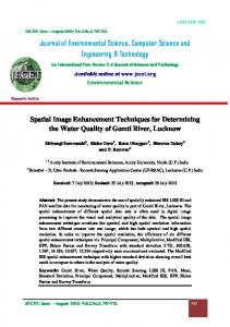
Figure 8: Output for different window size and sigma. Table 1. Shows the variation in Variance, Standard deviation and mean of resultant images with respect to Standard deviation of the LOG operator. The Table 1 shows the variation in Mean and Variance of output images with respect to the Standard deviation of the LOG operator, and these parameters are plotted in the Figure 9. Shown below. The plot shows that the variance and the mean of the resultant images decrease as the standard deviation of Gaussian operator increases.
Figure 9: Variation in Mean and Variance of output images with respect to the Standard deviation of the LOG operator.
Image Enhancement in Spatial domain by using LOG Operator
545
Table 1: Variance, Standard deviation and mean of resultant images with respect to Standard deviation of the LOG operator. Sigma(operator) 0.1 0.2 0.3 0.4 0.5 0.51 0.52 0.53 0.54 0.55 0.6 0.7 0.8 0.9 1 2 3 4
Sigma(o/p) 98.3055 98.2403 97.7843 95.5721 80.0458 77.2132 74.5473 72.1631 70.1561 68.4914 63.5368 61.3999 61.2499 61.2746 61.3273 61.7073 61.8477 61.9379
Mean(o/p) 176.8526 176.507 174.5098 166.2386 139.1432 135.6461 132.4689 129.717 127.4487 125.6164 121.0828 120.1181 119.7651 119.373 119.0437 117.8639 117.5479 117.3951
Variance(o/p) 9663.9713 9651.1565 9561.7693 9134.0262 6407.33 5961.8782 5557.2999 5207.513 4921.8783 4691.0718 4036.9249 3769.9477 3751.5502 3754.5766 3761.0377 3807.7908 3825.1379 3836.3034
Conclusion & Future Scope Using the proposed algorithm contrast has been increased considerably. The Laplacian operator is a 2-D isotropic measure of the 2nd spatial derivative of an image. The Laplacian of an image highlights regions of rapid intensity change and is therefore often used for edge detection. The Laplacian is often applied to an image that has first been smoothed with something approximating a Gaussian smoothing filter in order to reduce its sensitivity to noise. But this paper explains how we can achieve enhancement of images by using the LOG operator. I.e. If a portion of the filtered, or gradient, image is added to the original image, then the Resultant image having more contrast. ie Using LOG approach contrast has been increased considerably. Another most important conclusion is that from the graph it is evident that variance and the mean of the resultant images reduce significantly as standard deviation of LOG operator increases. Futue extension may be using frequency domain approach.
546
Vikrant Singh Thakur et al
References [1]
[2] [3] [4] [5]
[6] [7] [8]
[9]
[10]
[11]
Rafael C. Gonzalez, “Digital image processing”, 2nd edition, Fourth Indian Reprint, Richard E. Woods, Singapore: Pearson Education, 2003, pp. 75142. Anil K.Jain, “Fundamentals of Image Processing”, Fourth Indian Reprint, Sing apore: Pearson Education, 2005, pp. 255-287. G.R. Sinha and D.R. Hardaha, “Fourier techniques in Image enhancement”, in Proc. ICNFT, SAASTRA, 2004, pp.1-6. M. Erdogan, “Measurement of Polished rock surface brightness by image analysis method”, Engineering Geology, vol.57, pp. 65-72, June 2000. Doron Shaked and Ingeborg Tastl, “Sharpness Measure: Towards Automatic I mage Enhancement”, in Proc. IEEE International Conference on Image Processing, 2005, pp. 11-14. M Analoui, “Radiographic image enhancement: spatial domainTechniques”, Dent maxillofacial Radiology, Vol. 30, pp. 1-9, 2000. Rudra Pratap, “MATLAB: A quick introduction for scientists and engineers”, version 6, Oxford University Press, 2002. N.K. Bose, Nilesh and A. Ahuja, Superresolution and noise filtering using moving least squares, IEEE transactions on Image Processing, Vol. 15, No. 8, p. 2239-2248, August 2006. Murat Balci and Hassan Foroosh, Subpixel estimation of shifts directly in the Fourier domain, IEEE transactions on Image Processing, Vol. 15, No. 7, p. 1965-1972, July 2006. James Z. Wang , Wavelets and Imaging Informatics: A Review of the Literature, Journal of Biomedical Informatics, Volume 34, Issue 2, p. 129-14, April 2001. E Srinivasan and D. Ebenezer, New nonlinear filtering strategies for eliminating medium and long tailed noise in images with edge preservation properties, IETE journal of Education, Vol. 46, No. 1, p. 3-11, Jan-March 2005.