given intensity image f, consider the m à n neighborhood of pixel p ..... R. Gonzales and R.E. Woods, Digital Image Processing,. Prentice Hall, 3rd edition, 2007.
Image Processing Prof. Christian Bauckhage
outline lecture 15
recap
non-linear filters median filter morphological operations
summary
recap
given intensity image f , consider the m × n neighborhood of pixel p at coordinate [x, y]
� Nxy = f [i, j] x − m2 6 i 6 x + m2 ∧ y − 2n 6 j 6 y + n2
we also write � Nxy = p0 , p1 , . . . , pq−1 y
where q = mn
x
recap
the mean or average intensity of all pixels in Nxy is
ˆp =
1 X 1 X pi = pi mn q pi ∈Nxy
i
if we compute this local mean for every coordinate [x, y] in f to create a new image g, the operation g[x, y] ← ˆp is called mean filtering
note
we may just as well compute a weighted mean filter P i wi pi g[x, y] ← P i wi
and we observe that the familiar Gaussian filter is but a specific weighted mean filter
recap
using convolutions, na¨ıve mean filtering requires � O m · n per pixel exploiting � separability, the effort reduces to O m + n per pixel using � integral images, we can even achieve O 1 per pixel
� O 1 computation of means using integral images
if x+ m 2
n
y+ 2 X X f [i, j] c[x, y, m, n] = m n mn
and
C[x, y] =
y x X X
c[i, j]
i=0 j=0
i=x− 2 j=y− 2
then � � � � c[x, y, m, n] = C x + m2 , y + 2n − C x + m2 , y − 2n − 1 � � � − C x − m2 − 1, y + 2n + C x − m2 − 1, y −
C
β
c y
C
−1
x
C c
y
x
�
α
c γ
δ
x
C c y
y
n 2
x
dynamic program to compute integral images
integral images can be computed in one pass C[x, y] = c[x, y] + C[x, y − 1] + C[x − 1, y] − C[x − 1, y − 1]
y
x
y
y
x
y
x
y
x
x
non-linear filters
once again: pixel neighborhoods
given intensity image f , consider the m × n neighborhood of pixel p at coordinate [x, y]
� Nxy = f [i, j] x − m2 6 i 6 x + m2 ∧ y − 2n 6 j 6 y + n2
we also write � Nxy = p0 , p1 , . . . , pq−1 y
where q = mn
x
median (of an ordered set)
now, assume that we order the set Nxy ascendingly � Rxy = r0 , r1 , . . . , rq−1 ri 6 ri+1 ∧ ri ∈ Nxy the element r q−1 is then called the median of Nxy 2
median (of an ordered set)
now, assume that we order the set Nxy ascendingly � Rxy = r0 , r1 , . . . , rq−1 ri 6 ri+1 ∧ ri ∈ Nxy the element r q−1 is then called the median of Nxy 2
if we compute the local median for every coordinate [x, y] in f to create a new image g, the operation g[x, y] ← r q−1 2
is called median filtering
didactic example (1)
local 3 × 3 neighborhood Nxy
···
.. . 128 233 245 121 242 240 · · · 118 127 231 .. .
corresponding ordered set Rxy � 118, 121, 127, 128, 231, 233, 240, 242, 235
didactic example (1)
local 3 × 3 neighborhood Nxy
···
.. . 128 233 245 121 242 240 · · · 118 127 231 .. .
corresponding ordered set Rxy and median � 118, 121, 127, 128, 231, 233, 240, 242, 235
didactic example (2)
local 3 × 3 neighborhood Nxy
···
.. . 0 0 0 0 1 0 ··· 0 1 1 .. .
corresponding ordered set Rxy � 0, 0, 0, 0, 0, 0, 1, 1, 1
didactic example (2)
local 3 × 3 neighborhood Nxy
···
.. . 0 0 0 0 1 0 ··· 0 1 1 .. .
corresponding ordered set Rxy and median � 0, 0, 0, 0, 0, 0, 1, 1, 1
example
import numpy as np import scipy.misc as msc import scipy.ndimage as img f = msc.imread(’cat.png’).astype(’float’) for m in [3, 5, 9, 15, 23, 33, 45]: g = img.median_filter(f, (m,m), mode=’constant’, cval=0.0) msc.toimage(g,cmin=0,cmax=255).save(’cat-med-%dx%d.png’ % (m,m))
example
original
3 × 3 median
5 × 5 median
9 × 9 median
15 × 15 median
23 × 23 median
33 × 33 median
45 × 45 median
algorithm 1: na¨ıve median
for all y = 0 . . . M − 1
average effort per pixel � O q log q
for all x = 0 . . . N − 1 sanity check for x and y Nxy = ∅ for all j =
rather slow whenever q = mn
− m2
...
m 2
for all i = − n2 . . . 2n
� �� Nxy = Nxy ∪ f y + j, x + i Rxy = qsort Nxy g[y, x] ← r q−1 2
�
is large
observation
the median is the 0.5 quantile of a given distribution
p(x)
x P (x)
1 2
med{p(x)}
x
histogram
a histogram H[i] is used to count “things” e.g. the number of occurrences of intensity i in an image note that, when normalized such that its entries sum to one, a histogram becomes a probability mass function
H[i]
C[i] =
Pi k=0
H[k]
algorithm 2: Huang, 1979
for all y = 0 . . . M − 1 for all x = 0 . . . N − 1 sanity check for x and y if [y, x] is upper left corner initialize histogram H else for all k = − n2 . . . n2 sub f [y + k, x − 2n − 1] from H add f [y + k, x + 2n ] to H P q = i H[i] s=0 for all i = 0 . . . #colors s = s + H[i] if s > q/2 median = i break
sketch
y
−
+
x
effort per pixel O(n) + 256 ops max = O(n) + O(1) = O(n)
observation
for disjoint sets A and B, we have H(A ∪ B) = H(A) + H(B) ⇒ idea: maintain a histogram hx for each column x of f
´ algorithm 3: Perreault & Hebert, 2007
for all y = 0 . . . M − 1 for all x = 0 . . . N − 1 sanity check for x and y if y is uppermost row initialize hx if [y, x] is upper left corner initialize H else sub f [y − m2 − 1, x + n2 ] from hx+ n 2 add f [y + m2 , x + n2 ] to hx+ n 2 H = H − hx− n −1 + hx+ n 2
sketch − y
+
x
2
s=0 .. . y
−
+
x
´ algorithm 3: Perreault & Hebert, 2007
effort per pixel (8-bit gray scale image) 1 addition and 1 subtraction for hx+ n2 256 additions and 256 subtractions for H = H − hx− 2n −1 + hx+ 2n max. 256 operations for computing s ⇒ O(1)
´ algorithm 3: Perreault & Hebert, 2007
effort per pixel (8-bit gray scale image) 1 addition and 1 subtraction for hx+ n2 256 additions and 256 subtractions for H = H − hx− 2n −1 + hx+ 2n max. 256 operations for computing s ⇒ O(1) yet, there is a large constant factor
´ algorithm 3: Perreault & Hebert, 2007
effort per pixel (8-bit gray scale image) 1 addition and 1 subtraction for hx+ n2 256 additions and 256 subtractions for H = H − hx− 2n −1 + hx+ 2n max. 256 operations for computing s ⇒ O(1) yet, there is a large constant factor however, additional neat tricks keep the effort low multilevel histograms addition / subtraction by means of bit shifting
´ algorithm 3: Perreault & Hebert, 2007
effort per pixel (8-bit gray scale image) 1 addition and 1 subtraction for hx+ n2 256 additions and 256 subtractions for H = H − hx− 2n −1 + hx+ 2n max. 256 operations for computing s ⇒ O(1) yet, there is a large constant factor however, additional neat tricks keep the effort low multilevel histograms addition / subtraction by means of bit shifting a corresponding implementation is available within OpenCV
morphology (1) � given f [x, y] and ordered set Rxy = ri ∈ Nxy ri 6 ri+1 the operation g[x, y] ← r0 is called erosion the operation g[x, y] ← rq−1 is called dilation
morphology (2)
erosion and dilation are useful in binary image processing they shrink or expand shapes (convention: � = 0, � = 1)
shape f
erosion e( f )
dilation d( f )
morphology (3)
extracting the boundary of a shape
shape f
boundary f − e( f )
morphology (4)
the operation d◦e is called opening the operation e◦d is called closing
morphology (5)
these remove isolated pixels or close holes
shape f
opening d e( f )
�
closing e d( f )
�
note
morphological operations are of importance in industrial computer vision (machine vision) and in medical image processing they are treated in great detail in R. Gonzales and R.E. Woods, Digital Image Processing, Prentice Hall, 3rd edition, 2007 ¨ B. Jahne, Digital Image Processing, Springer, 6th edition, 2005
note
to get an idea as to how to do binary morphology with Python/NumPy/SciPy, read C. Bauckhage, NumPy / SciPy Recipes for Image Processing: Binary Images and Morphological Operations, dx.doi.org/10.13140/RG.2.2.16622.00324
summary
we now know about
the median and median filtering efficient algorithms for median filtering morphological operations and possible applications