niques (Horn & Schunck (1981)) and matching techniques (Barron et al. (1994)). A widely used differential algorithm (Lucas & Kanade (1981)) that gives good ...
Image Stabilization in Active Robot Vision
261
14 1 Image Stabilization in Active Robot Vision Angelos Amanatiadis1 , Antonios Gasteratos1 , Stelios Papadakis2 and Vassilis Kaburlasos2 1 Democritus
2 Technological
University of Thrace Educational Institution of Kavala Greece
1. Introduction Recent demands in sophisticated mobile robots require many semi-autonomous or even autonomous operations, such as decision making, simultaneous localization and mapping, motion tracking and risk assessment, while operating in dynamic environments. Most of these capabilities depend highly on the quality of the input from the cameras mounted on the mobile platforms and require fast processing times and responses. However, quality in robot vision systems is not given only by the quantitative features such as the resolution of the cameras, the frame rate or the sensor gain, but also by the qualitative features such as sequences free of unwanted movement, fast and good image pre-processing algorithms and real-time response. A robot having optimal quantitative features for its vision system cannot achieve the finest performance when the qualitative features are not met. Image stabilization is one of the most important qualitative features for a mobile robot vision system, since it removes the unwanted motion from the frame sequences captured from the cameras. This image sequence enhancement is necessary in order to improve the performance of the subsequently complicated image processing algorithms that will be executed. Many image processing applications require stabilized sequences for input while other present substantially better performance when processing stabilized sequences. Intelligent transportation systems equipped with vision systems use digital image stabilization for substantial reduction of the algorithm computational burden and complexity (Tyan et al. (2004)), (Jin et al. (2000)). Video communication systems with sophisticated compression codecs integrate image stabilization for improved computational and performance efficiency (Amanatiadis & Andreadis (2008)), (Chen et al. (2007)). Furthermore, unwanted motion is removed from medical images via stabilization schemes (Zoroofi et al. (1995)). Motion tracking and video surveillance applications achieve better qualitative results when cooperating with dedicated stabilization systems (Censi et al. (1999)), (Marcenaro et al. (2001)), as shown in Fig. 1. Several robot stabilization system implementations that use visual and inertial information have been reported. An image stabilization system which compensates the walking oscillations of a biped robot is described in (Kurazume & Hirose (2000)). A vision and inertial cooperation for stabilization have been also presented in (Lobo & Dias (2003)) using a fusion model for the vertical reference provided by the inertial sensor and vanishing points from images. A visuo-inertial stabilization for space variant binocular systems has been also developed in (Panerai et al. (2000)), where an inertial device measures angular velocities and linear accelerations, while image geometry facilitates the computation of first-order motion parameters. In
262
Robot Vision
(a)
(b)
(c)
(d)
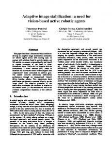
Fig. 1. Performance of automatic license plate recognition system: a) sample frame, b) processed frame only by zooming algorithm, c) processed frame only by stabilization algorithm, d) processed frame by both stabilization and zooming algorithms. (Zufferey & Floreano (2006)), course stabilization and collision avoidance is achieved using a bioinspired model of optic flow and inertial information applied to autonomous flying robots.
2. Image Stabilization Image stabilization schemes can be classified into three major categories. The optical image stabilizer employs a prism assembly that moves opposite to the shaking of camera for stabilization (Cardani (2006)), (Tokyo (1993)). A two axis gyroscope is used to measure the movement of the camera, and a microcontroller directs that signal to small linear motors that move the image sensor, compensating for the camera motion. Other designs move a lens somewhere in the optical chain within the camera. The electronic image stabilizer compensates the image sequence by employing motion sensors to detect the camera movement for compensation (Oshima et al. (1989)), (Kinugasa et al. (1990)). Gyroscopes are still used to detect the jitter, but instead of altering the direction of the prism, the image is simply shifted in software by a certain number of pixels. Both electronic and optical image stabilizers are hardware dependent and require built-in devices such as inertial sensors and servo motors. The digital image
Image Stabilization in Active Robot Vision
Input Image Sequence
Local Motion Estimation
Global Motion Vector Estimation
263
Compensating Motion Vector Estimation
Image compensation
Stabilized Image Sequence
Fig. 2. Typical architecture of an image stabilization technique. stabilizer (DIS) does not need any mechanical or optical devices since the image compensation is made through image processing algorithms. This attribute makes it suitable for low cost electronics (Ko et al. (1999)), (Vella et al. (2002)), (Xu & Lin (2006)), (Pan & Ngo (2005)). The DIS comprises two processing units: the motion estimation unit and the motion compensation unit. The purpose of motion estimation unit is to estimate reliably the global camera movement through the local motion estimation vectors of the acquired image sequence. The effectiveness of a DIS is closely tied with the accuracy of detecting the local motion vectors, in order to produce the right global motion vector. Following motion estimation, the motion compensation unit generates the compensating motion vector and shifts the current picking window according to the compensating motion vector to obtain a smoother image sequence. Motion compensation can take up 10% of the total computation of a digital stabilizer (Chen et al. (2007)). Various algorithms have been developed to estimate the local motion vectors, such as representative point matching (Vella et al. (2002)), edge pattern matching (Paik et al. (1992)), block matching (Xu & Lin (2006)) and bit plane matching (Ko et al. (1999)). All the previous algorithms, despite their high accuracy and reliability, are strictly constrained to regular conditions exhibiting high sensitivity to various irregular conditions such as moving objects, intentional panning, sequences acquired in low signal-to-noise ratio or zooming. For moving objects, solutions have been proposed such as in (Erturk (2003)). For sequences acquired in low signal-to-noise ratio, a blind DIS with the use of genetic algorithms is proposed in (NaitAli (2007)). Intentional panning has also been greatly improved using background estimation (Hsu et al. (2005)). For zooming, CMOS digital image stabilization schemes have been proposed in (Cho et al. (2007)) and (Cho & Hong (2007)). However, due to the fact that they are based on the distortion effect caused by the rolling shuttering mechanism of the CMOS sensor, they are effective only in CMOS sensors. A typical architecture of a DIS is shown in Fig. 2. The motion estimation unit computes the motion between two consecutive frames. This is achieved firstly by the local motion estimation subunit, which estimates the local motion vectors within frame regions. Secondly, the global motion estimation unit determines the global motion vectors by processing the previously estimated local motion vectors. Following the motion estimation unit, the motion compensation unit firstly, generates the compensating motion vector and secondly, shifts the current picking window according to the compensating motion vector to obtain a free of high frequency image sequence but still keep the global ego-motion of the sequence.
3. Active robot vision The term active vision is used to describe vision systems, where the cameras do not stand still to observe the scene in a passive manner, but, by means of actuation mechanisms, they can aim towards the point of interest. The most common active stereo vision systems comprise
264
Robot Vision
a pair cameras horizontally aligned (Gasteratos et al. (2002)), (Samson et al. (2006)). In these systems the movement of the stereo rig is done by means of 2 degrees of freedom: one for the horizontal movement (pan) and the other for the vertical one (tilt); moreover each of the cameras obeys to an independent pan movement (vergence), which raises the total degrees of freedom of the system to four. To these apparatuses are often incorporated other sensors, such as gyros, accelerometers or acoustical ones (Lungarella et al. (2003)). The integration of other than visual sensors on an active stereo head is used as a supplementary source of information from the environment. They are utilized in additional feedback loops, in order to increase the system robustness. Such an application is the utilization of gyros for image stabilization and gaze control (Panerai et al. (2003)). When a robot with a vision system moves around its environment undesirable position fluctuations in its visual field might occur, due to its locomotion. It is apparent that such fluctuation degrades the robot’s visual functions and, thus, it is critical to avoid them, by stabilizing the images. In biological systems this is avoided owing to Vestibulo-Ocular Reflex (VOR), which derives from the brain and governs compensatory eye movements. However, in a teleoperated robot there is not any mean to wire the operator’s brain with the actuators on the robot head. In this case a local control loop should be applied, that replicates the VOR on the tele-operated head. Figure 3 depicts a rough block diagram of the closed-loop control scheme for the pan dof, which incorporates a look-ahead control loop for the external horizontal disturbance. The look-ahead control strategy is utilized to predict the image fluctuations due to abrupt disturbances on the stereo head. The horizontal component of the disturbance applied on the head is measured by the inertial sensor. This signal is then fed into the look-ahead controller, which produces a control signal for the controller of the pan degree of freedom ( Gc ). The controller Gc is a standard PID controller ( Gc = K p + Ksi + Kd × s), which produces a counteracting order to the actuator that moves the pan ( G p ). This way the rotational component of the horizontal disturbance is suppressed. At the final stage, the horizontal retinal slippage is computed on two sequential image frames using a differential technique. This is used as a feedback signal in a closed-loop that fine-tunes the image stabilization. An identical local control loop is utilized for vertical disturbance and the tilt (having the same PID parameters). Images are stabilized in two axes in this manner, and the operator’s suffering from fast image changes is compensated.
4. Evaluation measures Evaluation procedures for image stabilization algorithms and architectures are presented in (Engelsberg & Schmidt (1999)), (Morimoto & Chellappa (1998)) and (Balakirsky & Chellappa (1996)). In robot vision the factors that are more important in the image stabilization schemes are the accuracy of the system in terms of image quality and the displacement range in terms of pixels or degrees per second. The quality of a stabilized sequence can be measured with the help of the interframe transformation fidelity which is defined as the PSNR between two consecutive stabilized frames, which is given by: ITF =
1 N −1 PSNR( Ik , Ik+1 ) N − 1 k∑ =1
(1)
Image Stabilization in Active Robot Vision
265 R(s): Input D(s): Disturbance Gc : Controller Gp : Pan motor Gs : Look-ahead controller H : Horizontal retinal slippage
D(s) Gs
R(s)
+
-
Gc
+
+
Gp
Stabilized images
+ H
Fig. 3. Control scheme for compensation of the horizontal disturbances. The inertial sensors are used for a look-ahead mechanism, which directly measures the disturbance and provides a negative input to the controller. The horizontal component of the optic flow measured in both cameras is used as feedback to the system. with N the number of frames of the sequence. The PSNR between two consecutive frame Ik and Ik+1 is given by: � � MAX I (2) PSNR( Ik , Ik+1 ) = 20 × log10 RMSE( Ik , Ik+1 )
5. Case study A rotational and translational image stabilization system for a pan and tilt active stereo camera head will be presented. The system is designed to fit into mobile rover platforms allowing the architecture to be modular and the whole system expandable. Special attention was paid to the real-time constraints, particularly for the control part of the system. The stabilization system as shown in Fig. 4, consists of a stereo vision head (Gasteratos & Sandini (2001)), two high resolution digital cameras, a DSP inertial sensor, four actuators and controllers and two processing units. Pan and tilt compensation is achieved though mechanical servoing while vertical and horizontal compensation is achieved by frame shifting through a digital frame stabilization algorithm. A key feature is the real-time servo control system, written in C, using Open Source Software which includes a Linux-based Real-Time Operating System, a Universal Serial Bus to RS-232 serial driver, CAN bus drivers and an open source network communication protocol for the communication between the two processing units. 5.1 Hardware Architecture
The system functions can be separated into information processing and motion control. Information processing includes the gyrosensor output and the image processing. However, image processing presents a high computational burden and recourses while it demands the full usage of certain instruction sets of a modern microprocessor. In contrast, motion control requires the operation system to be able to execute real-time tasks. This demand for high multimedia performance and real-time motion control has forced us to adopt a computer structure consisting of a computer with Windows operating system for the image processing and a computer with RT-Linux operating system for the control tasks. The computers are connected to each other by a high speed network protocol for synchronization and frame compensation
266
Robot Vision
Fig. 4. The stereo head vision system. The modules shown here are: the stereo vision head with the fixed actuators, the two digital cameras, the inertial sensor and the four controllers. purposes. This inter-host communication protocol between the computers uses a higher level abstraction, built on top of sockets, meeting the requirements for low latency. The interfaces used are CAN bus for the controllers (Tindell et al. (1994)), USB 2.0 for the cameras a USB 1.0 to serial output for the inertial sensor. The drivers for the interfaces connected to the RT-Linux computer are open source under the General Public License. In order to fully utilize the advantages and precision of the modern digital servo drives a fine tuning process (Astrom & Hagglund (1995)) for the pan and tilt PID controllers was carried out. The tuning was orientated for position control and due to the different inertia load seen on the motor shaft of the pan and tilt axis the integral, derivative and proportional band values were set to different values for each axis respectively. In order to determine the internal camera geometric and optical characteristics, camera calibration was necessary. A variety of methods have been reported in the bibliography. The method we used is described in (Bouget (2001)) using its available C Open Source code. The method is a non self-calibrating thus, we used a projected chessboard pattern to estimate the camera intrinsics and plane poses. Finally, the calibration results were used to rectify the images taken from cameras in order to have the best results in the subsequent image processing algorithms. 5.2 Software Architecture
Key feature for the implementation of the real-time control is the operating system we used. Since critical applications such as control, need low response times, OCERA operating system (OCERA project home page (2008)) was chosen. OCERA is an Open Source project which provides an integrated execution environment for embedded real-time applications. It is based on components and incorporates the latest techniques for building embedded systems. OCERA architecture is designed to develop hybrid systems with hard and soft real-time activities as shown in Fig. 5. In this case, we allocated the critical task of control at the RTLinux level and the less critical tasks, such as inertial data filtering, at the Linux level. The interface for both kinds of activities is a POSIX based interface. For motion estimation, the rectified frames are processed with an optic flow method in order to extract the global motion translation vector for the motion compensation. The affine model
Image Stabilization in Active Robot Vision
267
Fig. 5. The chosen operating system combines the use of two kernels, Linux and RTLinux-GPL to provide support for critical tasks (RTLinux-GPL executive) and soft real-time applications (Linux kernel). of the optic flow that was used is described in (Koenderink & van Doorn (1991)) for the basis of frame translation, using a single camera input. For motion compensation process, the estimation method in (Hsu et al. (2005)) was selected, in order to remove the undesired shaking motion and simultaneously maintain the ego-motion of the stereo head. The digital inertial sensor consists of a compact sensor package, which includes accelerometers and gyros to measure accelerations and angular rates. The errors in the force measurements introduced by accelerometers and the errors in the measurement of angular change in orientation with respect to the inertial space introduced by gyroscopes are two fundamental error sources which affect the error behavior of the rotational stabilization. Furthermore, inertial measurements are corrupted by additive noise (Ovaska & Valiviita (1998)). The Kalman filter (Welch & Bishop (2001)), (Trucco & Verri (1998)) was used which is a form of optimal estimator, characterized by recursive evaluation using an estimated internal model of the dynamics of the system. The filtering is implemented on the RT-Linux computer where the inertial sensor is attached. Finally, the optimized filter outputs of pan and tilt are the subsequent feedback to the controllers for opposite movement of the pan and tilt axis, respectively. The concurrency and parallelism was considered in the programming of the robotic system by using a multi-thread model. The motor run time models are not using the wait.until.done() function, while a change in the operator’s field of view indicates that the previous movement should not be completed but a new motion position command should be addressed. Simultaneous and non-synchronized accesses to the same resources, such as servo motors, is a critical aspect since both stabilization and head tracking movement are performed at the same time, as shown in Fig. 6. Thus, a priority scheduling feedback loop (Locke (1992)) was implemented. The priority feedback scheduler is implemented as an additional real-time periodic task. The inputs are the measured response times of the control tasks and the inputs from both sensors. Priority was given to head posing tracker since we were interested firstly in giving the operator the desired view and then an optimized view by mechanical stabilization. The RT-Linux kernel keeps track of the real time tasks execution cycles, thus allowing to recover a precise measure of the control tasks execution times from the scheduling regulator. As
268
Robot Vision
Stabilization Command
Direction Command
Fig. 6. Concurrent movement commands are applied to the same axis. the feedback scheduler is a simple feedback algorithm running at a slow rate, its computing cost is quite low. The software programming infrastructure considered the shared resources and critical sections in order to guarantee the expandability and flexibility of the stereo vision system. The critical sections were easily implemented since the protected operations were limited. However, special attention was paid since critical sections can disable system interrupts and can impact the responsiveness of the operating system. 5.3 Algorithm Implementation 5.3.1 Kalman Filtering
¯ taking into Discrete Kalman filter computes the best estimate of the systems’s state at tk , x, account the state estimated by the system model at tk−1 and the measurement, zk , taken at tk . � The Kalman filter equations are characterized by the state covariance matrices, Pk and Pk , and � the gain matrix, Kk . Pk is the covariance matrix of the k-th state estimate �
x¯ k = Φk−1 x¯ k−1
(3)
predicted by the filter immediately before obtaining the measurement zk , where Φk−1 is a time dependent n × n matrix called state transition matrix. Pk is the covariance matrix of the k-th state estimate, x¯ k computed by the filter after integrating the measurement, zk , with � the prediction, x¯ k . The covariance matrices are a quantitative model of the uncertainty of � � xk and xk . Finally, Kk establishes the relative importance of the prediction, x¯ k , and the state measurement, x¯ k . Let Qk and Rk be the covariance matrices of the white, zero-mean, Gaussian system and measurement noise respectively. The Kalman filter equations are �
Pk = Φk−1 Pk−1 Φ� k −1 + Q k −1
(4)
Kk = Pk Hk� ( Hk Pk Hk� + Rk )−1
(5)
x¯ k = Φk−1 x¯ k−1 + Kk (zk − Hk Φk−1 x¯ k−1 )
(6)
�
�
�
Pk = ( I − Kk ) Pk ( I − Kk )
�
+ Kk Rk Kk�
(7)
Using (4) to (7), we estimate the state and its covariance recursively. Initial estimates of the covariance matrix P0 and of the state, x¯0 , were set to 0 and 1 respectively (Welch & Bishop (2001)). � First, Pk is estimated according to (4). Second, the gain of the Kalman filter is computed by (5), before reading the new inertial measurements. Third, the optimal state estimate at time tk , x¯ k , is formed by (6), which integrates the state predicted by the system model (Φk−1 x¯ k−1 ) with the discrepancy of prediction and observation (zk − Hk Φk−1 x¯ k−1 ) in a sum weighted by the gain matrix, Kk . Finally, the new state covariance matrix, Pk , is evaluated through (7). In our
Image Stabilization in Active Robot Vision
269
Fig. 7. Sample data during the experiment session. The input reference is 0.3deg/ses (black line), the output of the inertial sensor (crosses) and the filtered Kalman output (gray line).
√ inertial sensor, the calibrated rate of turn noise density is 0.1units/ Hz with units in deg/s. Operating in 40Hz bandwidth, the noise is 0.015deg/s. An experiment was carried out to quantify the filtering behavior of the system in real-time. We applied a recursive motion profile to the tilt axis with constant velocity of 0.3deg/sec. During the experiment the following parameters were stored to estimate the overall performance: (i) the velocity stimulus input reference (ii) position angle of the controlled tilt servo encoder, (iii) output of the inertial sensor and (iv) the Kalman filter output. Figure 7 shows the sample data recorded during the test session. As it can seen the Kalman filtered output is close to the input reference by estimating the process state at a time interval and obtaining feedback in the form of the noisy inertial sensor measurement. 5.3.2 Optic Flow and Motion Compensation
Techniques for estimating the motion field are divided in two major classes: differential techniques (Horn & Schunck (1981)) and matching techniques (Barron et al. (1994)). A widely used differential algorithm (Lucas & Kanade (1981)) that gives good results was chosen for implementation. Given the assumptions of the image brightness constancy equation yields a good approximation of the normal component of the motion filed and that motion field is well approximated by a constant vector field within any small patch of the image plane, for each point pi within a small, n × n patch, Q, we derive
(∇ E)� v + Et = 0
(8)
where spatial and temporal derivatives of the image brightness are computed at p1 , p2 , . . . , p N 2 , with E = E( x, y, t) the image brightness and v, the motion filed. Therefore, the optical flow can be estimated within Q as the constant vector, v, ¯ that minimizes the functional Ψ[v] = ∑ [(∇ E)� v + Et ]2 (9) pi ∈ Q
The solution to this least squares problem can be found by solving the linear system A� Av = A� b
(10)
270
Robot Vision
Fig. 8. Horizontal frame sample data during the experiment session. The input before stabilization (red line) and the output after stabilization (blue line) is demonstrated. The i-th row of the N 2 × 2 matrix A is the spatial image gradient evaluated at point pi A = [∇ E(p1 ), ∇ E(p2 ), . . . , ∇ E(p N × N )]�
(11)
and b is the N 2 -dimensional vector of the partial temporal derivatives of the image brightness, evaluated at p1 , p2 . . . p N 2 , after a sign change b = −[ Et (p1 ), Et (p2 ), . . . , Et (p N × N )]�
(12)
Finally, the optic flow v¯ at the center of patch Q can be obtained as v¯ = ( A� A)−1 A� b
(13)
Furthermore, we applied to each captured rectified image a Gaussian filter with a standard deviation of σs = 1.5. The filtering was both spatial and temporal in order to attenuate noise in the estimation of the spatial image gradient and prevent aliasing in the time domain. The patch used is 5 × 5 pixels and three consecutive frames are the temporal dimension. The algorithm is applied for each patch and only the optic flow for the pixel at the center of the patch is computed, generating a sparse motion field with high performance speed of 10 f rames/sec for 320 × 240 image resolution. The Global Motion Vector (GMV) is represented by the arithmetic mean of the local motion vectors in each of the patches and can be potentially effective when subtracting the ego-motion commands of the stereo head which are available through the servo encoders. Subsequently, the compensation motion vector estimation is used to generate the Compensating Motion Vectors (CMVs) for removing the undesired shaking motion but still keeping the steady motion
Image Stabilization in Active Robot Vision
271
Fig. 9. Vertical frame sample data during the experiment session. The input before stabilization (red line) and the output after stabilization (blue line) is demonstrated. of the image. The compensation motion vector estimation for the final frame shifting is given by (Paik et al. (1992)) CMV (t) = k (CMV (t − 1))
+ ( a GMV (t) + (1 − a) GMV (t − 1))
(14)
where t represents the frame number, 0 ≤ a ≤ 1 and k is a proportional factor for designating the weight between current frame stabilization and ego-motion. Finally, frame shifting is applied when both horizontal and vertical CMVs are determined. 5.4 System Performance
Due to the fact that rotational stabilization process runs on the RT-Linux computer we have succeeded its real-time operation. Thus, stabilization can be considered as two separate processes that operate independently, since the frame sequences captured from the camera have been already rotationally stabilized by the mechanical servoing. The horizontal and vertical stabilization experiments are demonstrated in Fig. 8 and Fig. 9, respectively. The results show a frame sequence free of high frequency fluctuations, maintaining though, the ego-motion of the trajectory. The overall system is capable of processing 320 × 240 pixel image sequences at approximately 10 f rames/sec, with a maximum acceleration of 4 deg/sec2 .
6. Conclusion In this chapter, we covered all the crucial features of image stabilization in active robot vision systems. The topics included real-time servo control approaches for the electronic image stabilization, image processing algorithms for the digital image stabilization, evaluation measures, and robot control architectures for hard and soft real-time processes. A case study of
272
Robot Vision
an active robot vision image stabilization scheme was also presented, consisting of a four degrees of freedom robotic head, two high resolution digital cameras, a DSP inertial sensor, four actuators and controllers and one processing unit. Pan and tilt compensation was achieved through mechanical servoing while vertical and horizontal compensation was achieved by frame shifting through a digital frame stabilization algorithm. key feature was the real-time servo control system, written in C, using Open Source Software which includes a Linux-based Real-Time Operating System, a Universal Serial Bus to RS-232 serial driver, CAN bus drivers and an open source network communication protocol for the communication between the two processing units.
7. References Amanatiadis, A. & Andreadis, I. (2008). An integrated architecture for adaptive image stabilization in zooming operation, IEEE Trans. Consum. Electron. 54(2): 600–608. Astrom, K. & Hagglund, T. (1995). PID controllers: Theory, Design and Tuning, Instrument Society of America, Research Triangle Park. Balakirsky, S. & Chellappa, R. (1996). Performance characterization of image stabilization algorithms, Proc. Int. Conf. Image Process., Vol. 1, pp. 413–416. Barron, J., Fleet, D. & Beauchemin, S. (1994). Performance of optical flow techniques, International Journal of Computer Vision 12(1): 43–77. Bouget, J. (2001). Camera calibration toolbox for Matlab, California Institute of Technology, http//www.vision.caltech.edu . Cardani, B. (2006). Optical image stabilization for digital cameras, IEEE Control Syst. Mag. 26(2): 21–22. Censi, A., Fusiello, A. & Roberto, V. (1999). Image stabilization by features tracking, Proc. Int. Conf. Image Analysis and Process., pp. 665–667. Chen, H., Liang, C., Peng, Y. & Chang, H. (2007). Integration of digital stabilizer with video codec for digital video cameras, IEEE Trans. Circuits Syst. Video Technol. 17(7): 801–813. Cho, W. & Hong, K. (2007). Affine motion based CMOS distortion analysis and CMOS digital image stabilization, IEEE Trans. Consum. Electron. 53(3): 833–841. Cho, W., Kim, D. & Hong, K. (2007). CMOS digital image stabilization, IEEE Trans. Consum. Electron. 53(3): 979–986. Engelsberg, A. & Schmidt, G. (1999). A comparative review of digital image stabilising algorithms for mobile video communications, IEEE Trans. Consum. Electron. 45(3): 591– 597. Erturk, S. (2003). Digital image stabilization with sub-image phase correlation based global motion estimation, IEEE Trans. Consum. Electron. 49(4): 1320–1325. Gasteratos, A., Beltran, C., Metta, G. & Sandini, G. (2002). PRONTO: a system for mobile robot navigation via CAD-model guidance, Microprocessors and Microsystems 26(1): 17–26. Gasteratos, A. & Sandini, G. (2001). On the accuracy of the Eurohead, Lira-lab technical report, LIRA-TR 2. Horn, B. & Schunck, B. (1981). Determining optical flow, Artificial Intelligence 17(1-3): 185–203. Hsu, S., Liang, S. & Lin, C. (2005). A robust digital image stabilization technique based on inverse triangle method and background detection, IEEE Trans. Consum. Electron. 51(2): 335–345. Jin, J., Zhu, Z. & Xu, G. (2000). A stable vision system for moving vehicles, IEEE Trans. on Intelligent Transportation Systems 1(1): 32–39.
Image Stabilization in Active Robot Vision
273
Kinugasa, T., Yamamoto, N., Komatsu, H., Takase, S. & Imaide, T. (1990). Electronic image stabilizer for video camera use, IEEE Trans. Consum. Electron. 36(3): 520–525. Ko, S., Lee, S., Jeon, S. & Kang, E. (1999). Fast digital image stabilizer based on gray-coded bit-plane matching, IEEE Trans. Consum. Electron. 45(3): 598–603. Koenderink, J. & van Doorn, A. (1991). Affine structure from motion, Journal of the Optical Society of America 8(2): 377–385. Kurazume, R. & Hirose, S. (2000). Development of image stabilization system for remote operation of walking robots, Proc. IEEE Int. Conf. on Robotics and Automation, Vol. 2, pp. 1856–1861. Lobo, J. & Dias, J. (2003). Vision and inertial sensor cooperation using gravity as a vertical reference, IEEE Trans. Pattern Anal. Mach. Intell. 25(12): 1597–1608. Locke, C. (1992). Software architecture for hard real-time applications: Cyclic executives vs. fixed priority executives, Real-Time Systems 4(1): 37–53. Lucas, B. & Kanade, T. (1981). An iterative image registration technique with an application to stereo vision, Proc. DARPA Image Understanding Workshop, Vol. 121, p. 130. Lungarella, M., Metta, G., Pfeifer, R. & Sandini, G. (2003). Developmental robotics: a survey, Connection Science 15(4): 151–190. Marcenaro, L., Vernazza, G. & Regazzoni, C. (2001). Image stabilization algorithms for videosurveillance applications, Proc. Int. Conf. Image Process., Vol. 1, pp. 349–352. Morimoto, C. & Chellappa, R. (1998). Evaluation of image stabilization algorithms, Proc. Int. Conf. Acoust., Speech, Signal Process., Vol. 5, pp. 2789–2792. Nait-Ali, A. (2007). Genetic algorithms for blind digital image stabilization under very low SNR, IEEE Trans. Consum. Electron. 53(3): 857–863. OCERA project home page (2008). http//www.ocera.org . Oshima, M., Hayashi, T., Fujioka, S., Inaji, T., Mitani, H., Kajino, J., Ikeda, K. & Komoda, K. (1989). VHS camcorder with electronic image stabilizer, IEEE Trans. Consum. Electron. 35(4): 749–758. Ovaska, S. & Valiviita, S. (1998). Angular acceleration measurement: A review, IEEE Trans. Instrum. Meas. 47(5): 1211–1217. Paik, J., Park, Y., Kim, D. & Co, S. (1992). An adaptive motion decision system for digital image stabilizer based on edge pattern matching, IEEE Trans. Consum. Electron. 38(3): 607– 616. Pan, Z. & Ngo, C. (2005). Selective object stabilization for home video consumers, IEEE Trans. Consum. Electron. 51(4): 1074–1084. Panerai, F., Metta, G. & Sandini, G. (2000). Visuo-inertial stabilization in space-variant binocular systems, Robotics and Autonomous Systems 30(1-2): 195–214. Panerai, F., Metta, G. & Sandini, G. (2003). Learning visual stabilization reflexes in robots with moving eyes, Neurocomputing 48: 323–338. Samson, E., Laurendeau, D., Parizeau, M., Comtois, S., Allan, J. & Gosselin, C. (2006). The agile stereo pair for active vision, Machine Vision and Applications 17(1): 32–50. Tindell, K., Hansson, H. & Wellings, A. (1994). Analysing real-time communications: Controller area network (CAN), Proc. 15 th Real-Time Systems Symposium, Citeseer, pp. 259–263. Tokyo, J. (1993). Control techniques for optical image stabilizing system, IEEE Trans. Consum. Electron. 39(3): 461–466. Trucco, E. & Verri, A. (1998). Introductory Techniques for 3-D Computer Vision, Prentice Hall PTR Upper Saddle River, NJ, USA.
274
Robot Vision
Tyan, Y., Liao, S. & Chen, H. (2004). Video stabilization for a camcorder mounted on a moving vehicle, IEEE Trans. on Vehicular Technology 53(6): 1636–1648. Vella, F., Castorina, A., Mancuso, M. & Messina, G. (2002). Digital image stabilization by adaptive block motion vectors filtering, IEEE Trans. Consum. Electron. 48(3): 796–801. Welch, G. & Bishop, G. (2001). An introduction to the Kalman filter, ACM SIGGRAPH 2001 Course Notes . Xu, L. & Lin, X. (2006). Digital image stabilization based on circular block matching, IEEE Trans. Consum. Electron. 52(2): 566–574. Zoroofi, R., Sato, Y., Tamura, S. & Naito, H. (1995). An improved method for MRI artifact correction due to translational motion in the imaging plane, IEEE Trans. on Medical Imaging 14(3): 471–479. Zufferey, J. & Floreano, D. (2006). Fly-inspired visual steering of an ultralight indoor aircraft, IEEE Trans. Robot. Autom. 22(1): 137–146.