May 18, 2011 - NA] 18 May 2011 ... sub-gradient methods [1,13], second-order cone programming (SOCP) [18], duality- based methods [8,11,22], and ...
Noname manuscript No. (will be inserted by the editor)
Implementation of an Optimal First-Order Method for Strongly Convex Total Variation Regularization
arXiv:1105.3723v1 [math.NA] 18 May 2011
T. L. Jensen · J. H. Jørgensen · P. C. Hansen · S. H. Jensen
Received: date / Accepted: date
Abstract We present a practical implementation of an optimal first-order method, due to Nesterov, for large-scale total variation regularization in tomographic reconstruction, image deblurring, etc. The algorithm applies to µ-strongly convex objective functions with L-Lipschitz continuous gradient. In the framework of Nesterov both µ and L are assumed known – an assumption that is seldom satisfied in practice. We propose to incorporate mechanisms to estimate locally sufficient µ and L during the iterations. The mechanisms also allow for the application to non-strongly convex functions. We discuss the iteration complexity of several first-order methods, including the proposed algorithm, and we use a 3D tomography problem to compare the performance of these methods. The results show that for ill-conditioned problems solved to high accuracy, the proposed method significantly outperforms state-of-theart first-order methods, as also suggested by theoretical results. Keywords Optimal first-order optimization methods · strong convexity · total variation regularization · tomography Mathematics Subject Classification (2000) 65K10 · 65R32 1 Introduction Large-scale discretizations of inverse problems [20] arise in a variety of applications such as medical imaging, non-destructive testing, and geoscience. Due to the inherThis work is part of the project CSI: Computational Science in Imaging, supported by grant no. 274-070065 from the Danish Research Council for Technology and Production Sciences. Tobias Lindstrøm Jensen, Søren Holdt Jensen Department of Electronic Systems, Aalborg University, Niels Jernesvej 12, 9220 Aalborg Ø, Denmark. E-mail: {tlj,shj}@es.aau.dk Jakob Heide Jørgensen, Per Christian Hansen Department of Informatics and Mathematical Modelling, Technical University of Denmark, Building 321, 2800 Lyngby, Denmark. E-mail: {jakj,pch}@imm.dtu.dk
2
T. L. Jensen, J. H. Jørgensen, P. C. Hansen, and S. H. Jensen
ent instability of these problems, it is necessary to apply regularization in order to compute meaningful reconstructions, and this work focuses on the use of total variation which is a powerful technique when the sought solution is required to have sharp edges (see, e.g., [12, 33] for applications in image reconstruction). Many total variation algorithms have already been developed, such as time marching [33], fixed-point iteration [37], and various minimization-based methods such as sub-gradient methods [1, 13], second-order cone programming (SOCP) [18], dualitybased methods [8, 11, 22], and graph-cut methods [9, 16]. The difficulty of a problem depends on the linear operator to be inverted. Most methods are dedicated to denoising, where the operator is simply the identity, or possibly deblurring of a simple blur, where the operator is invertible and represented by a fast transform. For general linear operators with no exploitable structure, such as in tomographic reconstruction, the selection of algorithms is limited. Furthermore, the systems that arise in real-world tomography applications, especially in 3D, are so large that memory-requirements preclude the use of second-order methods with quadratic convergence. Recently, Nesterov’s optimal first-order method [27, 28] has been adapted to, and analyzed for, a number of imaging problems [14, 38]. In [38] it is shown that Nesterov’s method outperforms standard first-order methods by an order of magnitude, but this analysis does not cover tomography problems. A drawback of Nesterov’s algorithm (see, e.g., [10]) is the explicit need for the strong convexity parameter and the Lipschitz constant of the objective function, both of which are not available in practice. This paper describes a practical implementation of Nesterov’s algorithm, augmented with efficient heuristic methods to estimate the unknown Lipschitz constant and strong convexity parameter. The Lipschitz constant is handled using backtracking, similar to the technique used in [4]. To estimate the unknown strong convexity parameter – which is more difficult – we propose a heuristic based on adjusting an estimate of the strong convexity parameter using a local strong convexity inequality. Furthermore, we equip the heuristic with a restart procedure to ensure convergence in case of an inadequate estimate. We call the algorithm UPN (Unknown Parameter Nesterov) and compare it with two versions of the well-known gradient projection algorithm; GP: a simple version using a backtracking line search for the stepsize and GPBB: a more advanced version using Barzilai-Borwein acceleration [2] and with the backtracking procedure from [19]. We also compare with a variant of the proposed algorithm, UPN0 , where the strong convexity information is not enforced. This variant is similar to the FISTA algorithm [4]. We have implemented the four algorithms in C with a MEX interface to MATLAB, and the software is available from www2.imm.dtu.dk/~pch/TVReg/. Our numerical tests demonstrate that the proposed method UPN is significantly faster than GP, and as fast as GPBB for moderately ill-conditioned problems, and significantly faster for ill-conditioned problems. Compared to UPN0 , UPN is consistently faster, when solving to high accuracy. We start with introductions to the discrete total variation problem, to smooth and strongly convex functions, and to some basic first-order methods in Sections 2, 3, and 4, respectively. Section 5 introduces important inequalities while the new algorithm
A First-Order Method for Strongly Convex TV Regularization
3
is described in Section 6. The 3D tomography test problem is introduced in Section 7. Finally, in Section 8 we report our numerical tests and comparisons. Throughout the paper we use the following notation. The smallest singular value of a matrix A is denoted σmin (A). The smallest and largest eigenvalues of a symmetric semi-definite matrix M are denoted by λmin (M) and λmax (M). For an optimization problem, f is the objective function, x? denotes a minimizer, f ? = f (x? ) is the optimum objective, and x is called an ε-suboptimal solution if f (x) − f ? ≤ ε.
2 The Discrete Total Variation Reconstruction Problem The Total Variation (TV) of a real function X (t) with t ∈ Ω ⊂ R p is defined as T (X ) =
Z
k∇X (t)k2 dt.
(2.1)
Ω
Note that the Euclidean norm is not squared, which means that T (X ) is non-differentiable. In order to handle this we consider a smoothed version of the TV functional. Two common choices are to replace the Euclidean norm of the vector z by either (kzk22 + β 2 )1/2 or the Huber function ( kzk2 ≥ τ, kzk2 − 12 τ if (2.2) Φτ (z) = 1 2 else. 2τ kzk2 In this work we use the latter, which can be considered a prox-function smoothing [28] of the TV functional [5]; thus, the approximated TV functional is given by Tτ (X ) =
Z
Φτ (∇X ) dt.
(2.3)
Ω
In this work we consider the case t ∈ R3 . To obtain a discrete version of the TV reconstruction problem, we represent X (t) by an N = m × n × l array X, and we let x = vec(X). Each element or voxel of the array X, with index j, has an associated matrix (a discrete differential operator) D j ∈ R3×N such that the vector D j x ∈ R3 is the forward difference approximation to the gradient at x j . By stacking all D j we obtain the matrix D of dimensions 3N × N: D1 D = ... . (2.4) DN We use periodic boundary conditions in D, which ensures that only a constant x has a TV of 0. Other choices of boundary conditions could easily be implemented. When the discrete approximation to the gradient is used and the integration in (2.3) is replaced by summations, the discrete and smoothed TV function is given by N
Tτ (x) =
∑ Φτ (D j x).
j=1
(2.5)
4
T. L. Jensen, J. H. Jørgensen, P. C. Hansen, and S. H. Jensen
The gradient ∇Tτ (x) ∈ RN of this function is given by N
∇Tτ (x) =
∑ DTj D j x/ max{τ, kD j xk2 }.
(2.6)
j=1
We assume that the sought reconstruction has voxel values in the range [0, 1], so we wish to solve a bound-constrained problem, i.e., having the feasible region Q = {x ∈ RN | 0 ≤ x j ≤ 1}. Given a linear system A x ≈ b where A ∈ RM×N and N = mnl, we define the associated discrete TV regularization problem as x? = argmin φ (x), x∈Q
φ (x) = 21 kA x − bk22 + α Tτ (x),
(2.7)
where α > 0 is the TV regularization parameter. This is the problem we want to solve, for the case where the linear system of equations arises from discretization of an inverse problem. 3 Smooth and Strongly Convex Functions To set the stage for the algorithm development in this paper, we consider the convex optimization problem minx∈Q f (x) where f is a convex function and Q is a convex set. We recall that a continuously differentiable function f is convex if f (x) ≥ f (y) + ∇ f (y)T (x − y),
∀ x, y ∈ RN .
(3.1)
Definition 3.1 A continuously differentiable convex function f is said to be strongly convex with strong convexity parameter µ if there exists a µ ≥ 0 such that f (x) ≥ f (y) + ∇ f (y)T (x − y) + 12 µkx − yk22 ,
∀ x, y ∈ RN .
(3.2)
Definition 3.2 A continuously differentiable convex function f has Lipschitz continuous gradient with Lipschitz constant L, if f (x) ≤ f (y) + ∇ f (y)T (x − y) + 12 Lkx − yk22 ,
∀ x, y ∈ RN .
(3.3)
Remark 3.1 The condition (3.3) is equivalent [27, Theorem 2.1.5] to the more standard way of defining Lipschitz continuity of the gradient, namely, through convexity and the condition k∇ f (x) − ∇ f (y)k2 ≤ Lkx − yk2 , ∀ x, y ∈ RN . Remark 3.2 Lipschitz continuity of the gradient is a smoothness requirement on f . A function f that satisfies (3.3) is said to be smooth, and L is also known as the smoothness constant. The set of functions that satisfy (3.2) and (3.3) is denoted Fµ,L . It is clear that µ ≤ L and also that if µ1 ≥ µ0 and L1 ≤ L0 then f ∈ Fµ1 ,L1 ⇒ f ∈ Fµ0 ,L0 . Given fixed choices of µ and L, we introduce the ratio Q = L/µ (sometimes referred to as the “modulus of strong convexity” [25] or the “condition number for f ” [27]) which is an upper bound for the condition number of the Hessian matrix. The number Q plays a major role for the convergence rate of optimization methods we will consider.
A First-Order Method for Strongly Convex TV Regularization
5
Lemma 3.1 For the quadratic function f (x) = 21 kA x − bk22 with A ∈ RM×N we have � σmin (A)2 if rank(A) = N, L = kAk22 , µ = λmin (AT A) = (3.4) 0, else, and if rank(A) = N then Q = κ(A)2 , the square of the condition number of A. Proof Follows from f (x) = f (y) + (A y − b)T A(x − y) + 12 (x − y)T AT A(x − y), the second order Taylor expansion of f about y, where equality holds for quadratic f . � Lemma 3.2 For the smoothed TV function (2.5) we have L = kDk22 /τ,
µ = 0,
(3.5)
where kDk22 ≤ 12 in the 3D case. Proof The result for L follows from [28, Thm. 1] since the smoothed TV functional can be written as [5, 14] o n τ Tτ (x) = max uT Dx − kuk22 : kui k2 ≤ 1, ∀ i = 1, . . . , N u 2 with u = (uT1 , . . . , uTN )T stacked according to D. The inequality kDk22 ≤ 12 follows from a straightforward extension of the proof in the Appendix of [14]. For µ pick y = αe ∈ RN and x = β e ∈ RN , where e = (1, . . . , 1)T , and α 6= β ∈ R. Then we get Tτ (x) = Tτ (y) = 0, ∇Tτ (y) = 0 and obtain 2 1 2 µkx − yk2
≤ Tτ (x) − Tτ (y) − ∇Tτ (y)T (x − y) = 0,
and hence µ = 0.
�
Theorem 3.1 For the function φ (x) defined in (2.7) we have a strong convexity parameter µ = λmin (AT A) and Lipschitz constant L = kAk22 +α kDk22 /τ. If rank(A) < N then µ = 0, otherwise µ = σmin (A)2 > 0 and Q = κ(A)2 +
α kDk22 , τ σmin (A)2
(3.6)
where κ(A) = kAk2 /σmin (A) is the condition number of A. Proof Assume rank(A) = N and consider f (x) = g(x) + h(x) with g ∈ Fµg ,Lg and h ∈ Fµh ,Lh . Then f ∈ Fµ f ,L f , where µ f = µg + µh and L f = Lg + Lh . From µ f and L f and using Lemmas 3.1 and 3.2 with g(x) = 12 kA x − bk22 and h(x) = αTτ (x) we obtain the condition number for φ given in (3.6). If rank(A) < N then the matrix AT A has at least one zero eigenvalue, and thus µ = 0. � Remark 3.3 Due to the inequalities used to derive (3.6), there is no guarantee that the given µ and L are the tightest possible for φ . For rank(A) < N there exist problems for which the Hessian matrix is singular and hence µ = 0, but we cannot say if this is always the case.
6
T. L. Jensen, J. H. Jørgensen, P. C. Hansen, and S. H. Jensen
4 Some Basic First-Order Methods A basic first-order method is the gradient projection method of the form � � x(k+1) = PQ x(k) − θk ∇ f (x(k) ) , k = 0, 1, 2, . . . .
(4.1)
The following theorem summarizes the convergence properties. Theorem 4.1 Let f ∈ Fµ,L , θk = 1/L and x? ∈ Q be the constrained minimizer of f , then for the gradient method (4.1) we have f (x(k) ) − f ? ≤
L (0) kx − x? k22 . 2k
(4.2)
Moreover, if µ 6= 0 then � � µ �k f (x(k) ) − f ? ≤ 1 − f (x(0) ) − f ? . L Proof The two bounds follow from [36] and [25, §7.1.4], respectively.
(4.3) �
To improve the convergence of the gradient (projection) method, Barzilai and Borwein [2] suggested a scheme in which the step θk ∇ f (x(k) ) provides a simple and computationally cheap approximation to the Newton step (∇2 f (x(k) ))−1 ∇ f (x(k) ). For general unconstrained problems with f ∈ Fµ,L , possibly with µ = 0, non-monotone line search combined with the Barzilai-Borwein (BB) strategy produces algorithms that converge [32]; but it is difficult to give a precise iteration complexity for such algorithms. For � strictly quadratic unconstrained problems the BB strategy requires O Q log ε −1 iterations to obtain an � ε-suboptimal solution [15]. In [17] it was argued that, in practice, O Q log ε −1 iterations “is the best that could be expected”. This comment is also supported by the statement in [27, p. 69] that all “reasonable step-size rules” have the same iteration complexity as the standard gradient method. Note that the classic gradient method (4.1) has O(L/ε) complexity for f ∈ F0,L . To summarize, when using the BB strategy� we should not expect better complexity than O(L/ε) for f ∈ F0,L , and O Q log ε −1 for f ∈ Fµ,L . In Algorithm 1 we give the (conceptual) algorithm GPBB, which implements the BB strategy with non-monotone line search [6, 39] using the backtracking procedure from [19] (initially combined in [32]). The algorithm needs the real parameter σ ∈ [0, 1] and the nonnegative integer K, the latter specifies the number of iterations over which an objective decrease is guaranteed. An alternative approach is to consider first-order methods with optimal complexity. The optimal complexity is defined as the worst-case complexity for a first-order method applied to any problem in a certain class [25, 27] (there are also more technical aspects involving the problem dimensions and a black-box assumption). In this paper we focus on the classes F0,L and Fµ,L . Recently there has been a great deal of interest in optimal first-order methods for convex optimization problems with f ∈ Fp 0,L [3, 35]. For this class it is possible to reach an ε-suboptimal solution within O( L/ε) iterations. Nesterov’s methods can be used as stand-alone optimization algorithm, or in a composite objective setup
A First-Order Method for Strongly Convex TV Regularization
7
Algorithm 1: GPBB
1 2 3 4
input : x(0) , K output: x(k+1) θ0 = 1 ; for k = 0, 1, 2, . . . do // BB strategy if k > 0 then θk ←
5
kx(k) −x(k−1) k22 h x(k) −x(k−1) ,∇ f (x(k) )−∇ f (x(k−1) ) i
;
11
β ← 0.95 ; x¯ ← PQ (x(k) − β θk ∇ f (x(k) )) ; fˆ ← max{ f (x(k) ), f (x(k−1) ), . . . , f (x(k−K) )} ; while f (x) ¯ ≥ fˆ − σ ∇ f (x(k) )T (x(k) − x) ¯ do β ← β2 ; x¯ ← PQ (x(k) − β θk ∇ f (x(k) )) ;
12
x(k+1) ← x¯ ;
6 7 8 9 10
[4, 29, 35], in which case they are called accelerated methods (because the designer violates the black-box assumption). Another option is to apply optimal first-order methods to a smooth approximation of a non-smooth function leading to an algorithm with O (1/ε) complexity [28]; for practical considerations, see [5, 14]. Optimal methods specific for the function class Fµ,L with µ > 0 are also known [26, 27]; see also [29] for the composite objective version. However, these methods have gained little practical consideration; for example √ in [29]−1all� the simulations are conducted with µ = 0. Optimal methods require O Q log ε iterations while the � −1 classic gradient method requires O Q log ε iterations [25, 27]. For quadratic problems, the conjugate gradient method achieves the same iteration complexity as the optimal first-order method [25]. In Algorithm 2 we state the basic p optimal method Nesterov [27] with known µ and L; it requires an initial θ0 ≥ µ/L. Note that it uses two sequences of vectors, x(k) and y(k) . The convergence rate is provided by the following theorem. p 0 L−µ) Theorem 4.2 If f ∈ Fµ,L , 1 > θ0 ≥ µ/L, and γ0 = θ0 (θ1−θ , then for algorithm 0 Nesterov we have � � 4L γ0 (0) (0) ? ? 2 f (x(k) ) − f ? ≤ √ (4.4) √ 2 f (x ) − f + kx − x k2 . 2 (2 L + k γ0 ) Moreover, if µ 6= 0 r �k � � � µ γ0 f (x ) − f ≤ 1 − f (x(0) ) − f ? + kx(0) − x? k22 . L 2 (k)
?
(4.5)
Proof See [27, (2.2.19), Theorem 2.2.3] and Appendix A for an alternative proof. �
8
T. L. Jensen, J. H. Jørgensen, P. C. Hansen, and S. H. Jensen
Algorithm 2: Nesterov
1 2 3 4 5 6
input : x(0) , µ, L, θ0 output: x(k+1) y(0) ← x(0) ; for k = 0, 1, 2, . . . do � x(k+1) ← PQ y(k) − L−1 ∇ f (y(k) ) ; θk+1 ← positive root of θ 2 = (1 − θ )θk2 + µL θ ; βk ← θk (1 − θk )/(θk2 + θk+1 ) ; y(k+1) ← x(k+1) + βk (x(k+1) − x(k) ) ;
Except for different constants Theorem 4.2 mimics the result in Theorem 4.1, with the crucial differences that the denominator in (4.4) is squared and µ/L in (4.5) has a square root. Comparing the convergence rates in Theoremsp4.1 and 4.2, we see that the rates are linear but differ in the linear rate, Q−1 and Q−1 , respectively. For ill-conditioned problems, it is important whether the complexity is a function of √ Q or Q, see, e.g., [25, §7.2.8]. This motivates the interest in specialized optimal first-order methods for solving ill-conditioned problems.
5 First-Order Inequalities for the Gradient Map For unconstrained convex problems the (norm of) the gradient is a measure of how close we are to the minimum, through the first-order optimality condition, cf. [7]. For constrained convex problems minx∈Q f (x) there is a similar quantity, namely, the gradient map defined by �� Gν (x) = ν x − PQ x − ν −1 ∇ f (x) . (5.1) Here ν > 0 is a parameter and ν −1 can be interpreted as the step size of a gradient step. The function PQ is the Euclidean projection onto the convex set Q [27]. The gradient map is a generalization of the gradient to constrained problems in the sense that if Q = RN then Gν (x) = ∇ f (x), and the equality Gν (x? ) = 0 is a necessary and sufficient optimality condition [36]. In what follows we review and derive some important first-order inequalities which will be used to analyze the proposed algorithm. We start with a rather technical result. Lemma 5.1 Let f ∈ Fµ,L , fix x ∈ Q, y ∈ RN , and set x+ = PQ (y − L¯ −1 ∇ f (y)), where µ¯ and L¯ are related to x, y and x+ by the inequalities ¯ − yk22 , f (x) ≥ f (y) + ∇ f (y)T (x − y) + 12 µkx
(5.2)
¯ + − yk22 . f (x+ ) ≤ f (y) + ∇ f (y)T (x+ − y) + 21 Lkx
(5.3)
¯ − xk22 . f (x+ ) ≤ f (x) + GL¯ (y)T (y − x) − 12 L¯ −1 kGL¯ (y)k22 − 21 µky
(5.4)
Then
A First-Order Method for Strongly Convex TV Regularization
9
Proof Follows directly from [27, Theorem 2.2.7].
�
Note that if f ∈ Fµ,L , then in Lemma 5.1 we can always select µ¯ = µ and L¯ = L to ensure that the inequalities (5.2) and (5.3) are satisfied. However, for specific x, y and x+ , there can exist µ¯ ≥ µ and L¯ ≤ L such that (5.2) and (5.3) hold. We will use these results to design an algorithm for unknown parameters µ and L. The lemma can be used to obtain the following lemma. The derivation of the bounds is inspired by similar results for composite objective functions in [29], and the second result is similar to [27, Corollary 2.2.1]. Lemma 5.2 Let f ∈ Fµ,L , fix y ∈ RN , and set x+ = PQ (y − L¯ −1 ∇ f (y)). Let µ¯ and L¯ be selected in accordance with (5.2) and (5.3) respectively. Then ? 1¯ 2 µky − x k2
≤ kGL¯ (y)k2 .
(5.5)
If y ∈ Q then 2 1 ¯ −1 2 L kGL¯ (y)k2
≤ f (y) − f (x+ ) ≤ f (y) − f ? .
(5.6)
Proof From Lemma 5.1 with x = x? we use f (x+ ) ≥ f ? and obtain ? 2 1¯ 2 µky − x k2
≤ GL¯ (y)T (y − x? ) − 12 L¯ −1 kGL¯ (y)k22 ≤ kGL¯ (y)k2 ky − x? k2 ,
and (5.5) follows; Eq. (5.6) follows from Lemma 5.1 using y = x and f ? ≤ f (x+ ). � As mentioned in the beginning of the section, the results of the corollary say that we can relate the norm of the gradient map at y to the error ky − x∗ k2 as well as to f (y) − f ∗ . This motivates the use of the gradient map in a stopping criterion: kGL¯ (y)k2 ≤ ε¯ ,
(5.7)
where y is the current iterate, and L¯ is linked to this iterate using (5.3). The parameter ε¯ is a user-specified tolerance based on the requested accuracy. Lemma 5.2 is also used in the following section to develop a restart criterion to ensure convergence.
6 Nesterov’s Method With Parameter Estimation The parameters µ and L are explicitly needed in Nesterov, but it is much too expensive to compute them explicitly; hence we need a scheme to estimate them during the iterations. To this end, we introduce the estimates µk and Lk of µ and L in each iteration k. We discuss first how to choose Lk , then µk , and finally we state the complete algorithm UPN and its convergence properties. To ensure convergence, the main inequalities (A.6) and (A.7) must be satisfied. Hence, according to Lemma 5.1 we need to choose Lk such that f (x(k+1) ) ≤ f (y(k) ) + ∇ f (y(k) )T (x(k+1) − y(k) ) + 21 Lk kx(k+1) − y(k) k22 .
(6.1)
This is easily accomplished using backtracking on Lk [4]. The scheme, BT, takes the form given in Algorithm 3, where ρL > 1 is an adjustment parameter. If the loop
10
T. L. Jensen, J. H. Jørgensen, P. C. Hansen, and S. H. Jensen
Algorithm 3: BT input : y, L¯ output: x, L˜ ˜ ← L¯ ; 1 L � ˜ −1 ∇ f (y) ; 2 x ← PQ y − L ˜ − yk22 do 3 while f (x) > f (y) + ∇ f (y)T (x − y) + 12 Lkx 4 L˜ ← ρL L˜ ; � 5 x ← PQ y − L˜ −1 ∇ f (y) ;
is executed nBT times, the dominant computational cost of BT is nBT + 2 function evaluations and 1 gradient evaluation. According to (A.7) with Lemma 5.1 and (A.8), we need to select the estimate µk such that µk ≤ µk? , where µk? satisfies f (x? ) ≥ f (y(k) ) + ∇ f (y(k) )T (x? − y(k) ) + 12 µk? kx? − y(k) k22 .
(6.2)
However, this is not possible because x? is, of course, unknown. To handle this problem, we propose a heuristic where we select µk such that f (x(k) ) ≥ f (y(k) ) + ∇ f (y(k) )T (x(k) − y(k) ) + 21 µk kx(k) − y(k) k22 .
(6.3)
This is indeed possible since x(k) and y(k) are known iterates. Furthermore, we want the estimate µk to be decreasing in order to approach a better estimate of µ. This can be achieved by the choice µk = min{µk−1 , M(x(k) , y(k) )}, where we have defined the function ( f (x)− f (y)−∇ f (y)T (x−y) 1 kx−yk2 2 2
M(x, y) = ∞
if
(6.4)
x 6= y,
(6.5)
else.
In words, the heuristic chooses the largest µk that satisfies (3.2) for x(k) and y(k) , as long as µk is not larger than µk−1 . The heuristic is simple and computationally inexpensive and we have found that it is effective for determining a useful estimate. Unfortunately, convergence of Nesterov equipped with this heuristic is not guaranteed, since the estimate can be too large. To ensure convergence we include a restart procedure RUPN that detects if µk is too large, inspired by the approach in [29, §5.3] for composite objectives. RUPN is given in Algorithm 4. To analyze the restart strategy, assume that µi for all i = 1, . . . , k are small enough, i.e., they satisfy µi ≤ µi? for i = 1, . . . , k, and µk satisfies f (x? ) ≥ f (x(0) ) + ∇ f (x(0) )T (x? − x(0) ) + 12 µk kx? − x(0) k22 .
(6.6)
A First-Order Method for Strongly Convex TV Regularization
11
Algorithm 4: RUPN γ1 = θ1 (θ1 L1 − µ1 )/(1 − θ1 ); if µk 6= 0 and inequality (6.9) not satisfied then 3 abort execution of UPN; 4 restart UPN with input (x(k+1) , ρµ µk , Lk , ε¯ ); 1 2
When this holds we have the convergence result (using (A.9)) �� � k � p f (x(1) ) − f ? + 12 γ1 kx(1) − x? k22 . f (x(k+1) ) − f ? ≤ ∏ 1 − µi /Li
(6.7)
i=1
We start from iteration k = 1 for reasons which will presented shortly (see Appendix A for details and definitions). If the algorithm uses a projected gradient step from the initial x(0) to obtain x(1) , the rightmost factor of (6.7) can be bounded as f (x(1) ) − f ? + 21 γ1 kx(1) − x? k22 ≤ GL0 (x(0) )T (x(0) −x? ) − 12 L0−1 kGL0 (x(0) )k22 + 12 γ1 kx(1) −x? k22 ≤ kGL0 (x(0) )k2 kx(0) −x? k2 − 12 L0−1 kGL0 (x(0) )k22 + 12 γ1 kx(0) −x? k22 � � 2 1 2γ1 ≤ − + kGL0 (x(0) )k22 . µk 2L0 µk2
(6.8)
Here we used Lemma 5.1, and the fact that a projected gradient step reduces the Euclidean distance to the solution [27, Theorem 2.2.8]. Using Lemma 5.2 we arrive at the bound r �� � k � 2 1 2γ1 µi (k+1) 2 1 ˜ −1 − + kGL0 (x(0) )k22 . (6.9) L kG (x )k ≤ 1 − ∏ 2 L˜ k+1 2 k+1 2 L µ 2L µ i 0 k i=1 k If the algorithm detects that (6.9) is not satisfied, it can only be because there was at least one µi for i = 1, . . . , k which was not small enough. If this is the case, we restart the algorithm with a new µ¯ ← ρµ µk , where 0 < ρµ < 1 is a parameter, using the current iterate x(k+1) as initial vector. The complete algorithm UPN (Unknown-Parameter Nesterov) is given in Algorithm 5. UPN is based on Nesterov’s optimal method where we have included backtracking on Lk and the heuristic (6.4). An initial vector x(0) and initial parameters µ¯ ≥ µ and L¯ ≤ L must be specified along with the requested accuracy ε¯ . The changes from Nesterov to UPN are at the following lines: 1: Initial projected gradient step to obtain the bound (6.8) and thereby the bound (6.9) used for the restart criterion. 5: Extra projected gradient step explicitly applied to obtain the stopping criterion kGL˜ k+1 (x(k+1) )k2 ≤ ε¯ . 6,7: Used to relate the stopping criterion in terms of ε¯ to ε, see Appendix B.3. 8: The heuristic choice of µk in (6.4).
12
T. L. Jensen, J. H. Jørgensen, P. C. Hansen, and S. H. Jensen
Algorithm 5: UPN
1 2 3 4 5 6 7 8 9 10 11 12
¯ ε¯ ¯ L, input : x(0) , µ, output: x(k+1) or x˜(k+1) ¯ ; [x(1) , L0 ] ← BT(x(0) , L) p ¯ µ0 = µ, y(1) ← x(1) , θ1 ← µ0 /L0 ; for k = 1, 2, . . . do [x(k+1) , Lk ] ← BT(y(k) , Lk−1 ) ; [x˜(k+1) , L˜ k+1 ] ← BT(x(k+1) , Lk ) ; if kGL˜ k+1 (x(k+1) )k2 ≤ ε¯ then abort, return x˜(k+1) ; if kGLk (y(k) )k2 ≤ ε¯ then abort, return x(k+1) ; � µk ← min µk−1 , M(x(k) , y(k) ) ; RUPN; θk+1 ← positive root of θ 2 = (1 − θ )θk2 + (µk /Lk ) θ ; βk ← θk (1 − θk )/(θk2 + θk+1 ) ; y(k+1) ← x(k+1) + βk (x(k+1) − x(k) ) ;
10: The restart procedure for inadequate estimates of µ. We note that in a practical implementation, the computational work involved in one iteration step of UPN may – in the worst case situation – be twice that of one iteration of GPBB, due to the two calls to BT. However, it may be possible to implement these two calls more efficiently than naively calling BT twice. We will instead focus on the iteration complexity of UPN given in the following theorem. ¯ ¯ Theorem p 6.1 Algorithm UPN, applied to f ∈ Fµ,L under conditions µ ≥ µ, L ≤ L, ε¯ = (µ/2) ε, stops using the gradient map magnitude measure and returns an εsuboptimal solution with iteration complexity �p � �p � O Q log Q + O Q log ε −1 . (6.10) Proof See Appendix B. � � √ The term O Q log Q in (6.10) follows from application of several inequalities involving the problem dependent parameters µ and L to obtain the overall bound� √ (6.9). Algorithm UPN is suboptimal since the optimal complexity is O Q log ε −1 but it has the advantage that it can be applied to problems with unknown µ and L.
7 The 3D Tomography Test Problem Tomography problems arise in numerous areas, such as medical imaging, non-destructive testing, materials science, and geophysics [21, 24, 30]. These problems amount to reconstructing an object from its projections along a number of specified directions,
A First-Order Method for Strongly Convex TV Regularization
13
Fig. 7.1 Left: Two orthogonal slices through the 3D Shepp-Logan phantom discretized on a 433 grid used in our test problems. Middle: Central horizontal slice. Right: Example of solution for α = 1 and τ = 10−4 . A less smooth solution can be obtained using a smaller α. Original voxel/pixel values are 0.0, 0.2, 0.3 and 1.0. Color range in display is set to [0.1, 0.4] for better constrast.
and these projections are produced by X-rays, seismic waves, or other “rays” penetrating the object in such a way that their intensity is partially absorbed by the object. The absorbtion thus gives information about the object. The following generic model accounts for several applications of tomography. We consider an object in 3D with linear attenuation coefficient X (t), with t ∈ Ω ⊂ R3 . The intensity decay bi of a ray along the line `i through Ω is governed by a line integral, Z bi = log(I0 /Ii ) =
`i
X (t) d` = bi ,
(7.1)
where I0 and Ii are the intensities of the ray before and after passing through the object. When a large number of these line integrals are recorded, then we are able to reconstruct an approximation of the function X (t). We discretize the problem as described in Section 2, such that X is approximated by a piecewise constant function in each voxel in the domain Ω = [0, 1]×[0, 1]×[0, 1]. Then the line integral along `i is computed by summing the contributions from all the voxels penetrated by `i . If the path length of the ith ray through the jth voxel is denoted by ai j , then we obtain the linear equations N
∑ ai j x j = bi ,
i = 1, . . . , M,
(7.2)
j=1
where M is the number of rays or measurements and N is the number of voxels. This is a linear system of equations A x = b with a sparse coefficient matrix A ∈ RM×N . A widely used test image in medical tomography is the “Shepp-Logan phantom,” which consists of a number superimposed ellipses. In the MATLAB function shepplogan3d [34] this 2D image is generalized to 3D by superimposing ellipsoids instead. The voxels are in the range [0, 1], and Fig. 7.1 shows an example with 43 × 43 × 43 voxels. We construct the matrix A for a parallel-beam geometry with orthogonal projections of the object along directions well distributed over the unit sphere, in order to obtain views of the object that are as independent as possible. The projection directions are the direction vectors of so-called Lebedev quadrature points on the unit
14
T. L. Jensen, J. H. Jørgensen, P. C. Hansen, and S. H. Jensen
sphere, and the directions are evenly distributed over the sphere; we use the MATLAB implementation getLebedevSphere [31]. For setting up the tomography system matrix for a parallel beam geometry, we use the Matlab implementation tomobox [23].
8 Numerical Experiments This section documents numerical experiments with the four methods UPN, UPN0 , GP and GPBB applied to the TV regularization problem (2.7). We use the two test problems listed in Table 8.1, which are representative across a larger class of problems (other directions, number of projections, noise levels, etc.) that we have run simulations with. The smallest eigenvalue of AT A for T1 is 2.19 · 10−5 (as computed by M ATLAB’s eigs), confirming that rank(A) = N for T1. We emphasize that this computation is only conducted to support the analysis of the considered problems since – as we have argued in the introduction – it carries a considerable computational burden to compute. In all simulations we create noisy data from an exact object xexact through the forward mapping b = Axexact +e, subject to additive Gaussian white noise of relative noise level kek2 /kbk2 = 0.01. As initial vector for the TV algorithms we use the fifth iteration of the iterative conjugate gradient method applied to the least squares problem. Table 8.1 Specifications of the two test problems; the object domain consists of m × n × l voxels and each projection is a p × p image. Any zero rows have been purged from A. Problem T1 T2
m=n=l 43 43
p 63 63
projections 37 13
dimensions of A 99361 × 79507 33937 × 79507
rank = 79507 < 79507
To investigate the convergence of the methods, we need the true minimizer x? with φ (x? ) = φ ? , which is unknown for the test problem. However, for comparison it is enough to use a reference solution much closer to the true minimizer than the iterates. Thus, to compare the accuracy of the solutions obtained with the accuracy parameter ε¯ , we use a reference solution computed with accuracy (ε¯ · 10−4 ), and with abuse of notation we use x? to denote this reference solution. We compare the algorithm UPN with GP (the gradient projection method (4.1) with backtracking line search on the step size), GPBB and UPN0 . The latter is UPN with µi = 0 for all i = 0, · · · , k and θ1 = 1. The algorithm UPN0 is optimal for the class F0,L and can be seen as an instance of the more general accelerated/fast proximal gradient algorithm (FISTA) with backtracking and the non-smooth term being the indicator function for the set Q, see [4, 3, 29] and the overview in [35].
8.1 Influence of α and τ on the convergence For a given A the theoretical modulus of strong convexity given in (3.6) varies only with α and τ. We therefore expect better convergence rates (4.3) and (4.5) for smaller α and larger τ. In Fig. 8.1 we show the convergence histories for T1 with all combinations of α = 0.01, 0.1, 1 and τ = 10−2 , 10−4 , 10−6 .
A First-Order Method for Strongly Convex TV Regularization
(φ(k)−φ*)/φ*
α = 0.01, τ = 0.01, α/τ =1e+00 0
10
GP GPBB UPN UPN0
−4
10
−8
10
0
α = 0.1, τ = 0.01, α/τ =1e+01 0
800
1200 1600 2000
−4
(φ(k)−φ*)/φ*
α = 0.01, τ = 0.0001, α/τ =1e+02 0
−8
400
800
1200 1600 2000
−4
0
1200 1600 2000
10
0
0
−8
1000 2000 3000 4000 5000
−4
0
10
α = 1, τ = 1e−06, α/τ =1e+06
−4
10
−8
Iteration k
2000 4000 6000 8000 10000
0
−4
1000 2000 3000 4000 5000
0
10
10
−8
10
α = 0.1, τ = 1e−06, α/τ =1e+05 10
10
1200 1600 2000
−4
0
10
800
10
−8
800
400
α = 1, τ = 0.0001, α/τ =1e+04 0
−4
400
0
10
10
−8
10
α = 0.1, τ = 0.0001, α/τ =1e+03
α = 0.01, τ = 1e−06, α/τ =1e+04 (φ(k)−φ*)/φ*
0
10
10
10
−4
10
0
10
10
10
10 10
α = 1, τ = 0.01, α/τ =1e+02 0
10
−8
400
15
0
−8
2000 4000 6000 8000 10000
Iteration k
10
0
4000 8000 12000 16000 20000
Iteration k
Fig. 8.1 Convergence histories (φ (x(k) ) − φ ? )/φ ? vs. k for T1 with α = 0.01, 0.1 and 1 and τ = 10−2 , 10−4 and 10−6 .
For low α/τ ratios, i.e., small condition number of the Hessian, GPBB and GP requires a comparable or smaller number of iterations than UPN and UPN0 . As α/τ increases, both GPBB and GP exhibit slower convergence, while UPN is less affected. In all cases UPN shows linear convergence, at least in the final stage, while UPN0 shows sublinear convergence. Due to these observations, we consistently observe that for sufficiently high accuracy, UPN requires the lowest number of itera−1 tions. This also follows from the theory since √ UPN scales as O(log ε ), whereas UPN0 scales at a higher complexity of O( ε −1 ). We conclude that for small condition numbers there is no gain in using UPN compared to GPBB. For larger condition numbers, and in particular if a high-accuracy solution is required, UPN converges significantly faster. Assume that we were to choose only one of the four algorithms to use for reconstruction across the condition number range. When UPN requires the lowest number of iterations, it requires significantly fewer, and when not, UPN only requires slightly more iterations than the best of the other algorithms. Therefore, UPN appears to be the best choice. Obviously, the choice of algorithm also depends on the demanded accuracy of the solution. If only a low accuracy, say (φ (k) − φ ? )/φ ? = 10−2 is sufficient, all four methods perform more or less equally well. 8.2 Restarts and µk and Lk histories To ensure convergence of UPN we introduced the restart functionality RUPN. In practice, we almost never observe a restart, e.g., in none of the experiments reported so far a restart occurred. An example where restarts do occur is obtained if we increase α to 100 for T1 (still τ = 10−4 ). Restarts occur in the first 8 iterations, and each time µk is reduced by a constant factor of ρµ = 0.7. In Fig. 8.2, left, the µk
16
T. L. Jensen, J. H. Jørgensen, P. C. Hansen, and S. H. Jensen
8
α = 100, τ = 0.0001, α/τ =1e+06
α = 1, τ = 0.0001, α/τ =1e+04 8
10
10
6
6
10
10
Lk
4
µk
4
10
5
10
10
Lk/µk
2
2
10
10
0
10
0
10
20 0
0
10
0
500
1000
1500
Iteration k
2000
10
0
500
1000
1500
2000
Iteration k
Fig. 8.2 The µk , Lk histories for T1. Left: α = 100 and τ = 10−4 . Right: α = 1 and τ = 10−4 .
and Lk histories are plotted vs. k and the restarts are seen in the zoomed inset as the rapid, constant decrease in µk . From the plot we also note that after the decrease in µk and an initial increase in Lk , both estimates are constant for the remaining iterations, indicating that the heuristics determines sufficient values. For comparison the µk and Lk histories for T1 with α = 1 and τ = 10−4 are seen in Fig. 8.2, right. No restarts occurred here, and µk decays gradually, except for one final jump, while Lk remains almost constant.
8.3 A non-strongly convex example Test problem T2 corresponds to only 13 projections, which causes A to not have full column rank. This leads to λmin (AT A) = 0, and hence φ (x) is not strongly convex. The optimal convergence rate is therefore given by (4.4); but how does the lack of strong convexity affect UPN, which was specifically constructed for strongly convex problems? UPN does not recognize that the problem is not strongly convex but simply relies on the heuristic (6.4) at the kth iteration. We investigate the convergence by solving T2 with α = 1 and τ = 10−4 . Convergence histories are given in Fig. 8.3, left. The algorithm UPN still converges linearly, although slightly slower than in the T1 experiment (α = 1, τ = 10−4 ) in Fig. 8.1. The algorithms GP and GPBB converge much more slowly, while at low accuracies UPN0 is comparable to UPN. But the linear convergence makes UPN converge faster for high accuracy solutions.
8.4 Influence of the heuristic An obvious question is how the use of the heuristic for estimating µ affects UPN compared to Nesterov, where µ (and L) are assumed known. From Theorem 3.1 we can compute a strong convexity parameter and a Lipschitz parameter for φ (x) assuming we know the largest and smallest magnitude eigenvalues of AT A. Recall that these µ and L are not necessarily the tightest possible, according to Remark 3.3. For T1 we have computed λmax (AT A) = 1.52 · 103 and λmin (AT A) = 2.19 · 10−5 (by
A First-Order Method for Strongly Convex TV Regularization
0
0
10
(φ(k)−φ*)/φ*
(φ(k)−φ*)/φ*
10
−4
10
−8
10
17
GP GPBB UPN UPN0
0
500
UPN UPN, µ and L
−4
10
−8
1000
Iteration k
1500
2000
10
0
500
1000
1500
2000
Iteration k
Fig. 8.3 Left: Convergence histories of GP, GPBB, UPN and UPN0 on T2 with α = 1 and τ = 10−4 . Right: Convergence histories of UPN and UPN using true µ and L on T1 with α = 1 and τ = 10−4 .
means of eigs in M ATLAB). Using α = 1, τ = 10−4 and kDk22 ≤ 12 from Lemma 3.2 we take α µ = λmin (AT A) = 2.19 · 10−5 , L = λmax (AT A) + 12 = 1.22 · 105 , τ and solve test problem T1 using UPN with the heuristics switched off in favor of these true strong convexity and Lipschitz parameters. Convergence histories are plotted in Fig. 8.3, right. The convergence is much slower than using UPN with the heuristics switched on. We ascribe this behavior to the very large modulus of strong convexity that arise from the true µ and L. It appears that UPN works better than the actual degree of strong convexity as measured by µ, by heuristically choosing in each step a µk that is sufficient locally instead of being restricted to using a globally valid µ. 9 Conclusion We presented an implementation of an optimal first-order optimization algorithm for large-scale problems, suited for functions that are smooth and strongly convex. While the underlying algorithm by Nesterov depends on knowledge of two parameters that characterize the smoothness and strong convexity, we have implemented methods that estimate these parameters during the iterations, thus making the algorithm of practical use. We tested the performance of the algorithm and compared it with two variants of the gradient projection algorithm and a variant of the FISTA algorithm. We applied the algorithms to total variation-regularized tomographic reconstruction of a generic threedimensional test problem. The tests show that, with regards to the number of iterations, the proposed algorithm is competitive with other first-order algorithms, and superior for difficult problems, i.e., ill-conditioned problems solved to high accuracy. Simulations also show that even for problems that are not strongly convex, in practice we achieve the favorable convergence rate associated with strong complexity. The software is available as a C-implementation with an interface to MATLAB from www2.imm.dtu.dk/~pch/TVReg/.
18
T. L. Jensen, J. H. Jørgensen, P. C. Hansen, and S. H. Jensen
A The Optimal Convergence Rate Here we provide an analysis of an optimal method for smooth, strongly convex functions without the use of estimation functions as in [27]. This approach is similar to the analysis of optimal methods for smooth functions in [35, 36]. The motivation for the following derivations is to introduce the iteration dependent Lk and µk estimates of L and µ. This will support the analysis of how Lk and µk should be selected. We start with the following relations to the “hidden” supporting variables z(k) and γk [27, pp. 73–75, 89], y(k) − x(k) = γk+1 = (1 − θk )γk + θk µk = θk2 Lk ,
θk γk (k) (z − y(k) ), γk+1
(A.1)
γk+1 z(k+1) = (1 − θk )γk z(k) + θk µk y(k) − θk GLk (y(k) ).
(A.2)
In addition we will make use of the relations γk+1 (k+1) 1 � kz − y(k) k22 = (1 − θk )2 γk2 kz(k) − y(k) k22 2 2γk+1 � −2θk (1 − θk )γk GLk (y(k) )T (z(k) − y(k) ) + θk2 kGLk (y(k) ))k22 ,
(A.3)
γk (1 − θk )γk θk µk 1 − (1 − θk )2 γk2 = . 2 2γk+1 2γk+1
(A.4)
(1 − θk )
which originate from (A.2). We will also later need the relation γk+1 (k+1) γk (k) kz − y(k) k22 − kz − y(k) k22 + θk GLk (y(k) )T (y(k) − x? ) 2 2 �T � γk+1 (k+1) γk kz − y(k) k22 + −γk+1 z(k+1) + (1 − θk )γk z(k) + θk µk y(k) (y(k) − x? ) (1 − θk ) kz(k) − y(k) k22 − 2 2 � � γk γk+1 γk γk+1 (k+1) T (k+1) (1 − θk ) − + θk µk (y(k) )T y(k) + (1 − θk ) (z(k) )T z(k) − (z ) z 2 2 2 2 + γk+1 (z(k+1) )T x? − (1 − θk )γk (z(k) )T x? − θk µk (y(k) )T x? � γ � � γk � (k) k+1 (1 − θk ) kz − x? k22 − (x? )T x? − kz(k+1) − x? k22 − (x? )T x? 2 2 � � � θk µk � (k) γk γk+1 θk µk ? 2 ? T ? + ky − x k2 − (x ) x + (1 − θk ) − + (y(k) )T y(k) 2 2 2 2 γk+1 (k) µk γk kz − x? k22 + θk ky(k) − x? k22 , (A.5) (1 + θk ) kz(k) − x? k22 − 2 2 2
(1 − θk ) = =
=
=
where we again used (A.2). We can now start the analysis of the algorithm by considering the inequality in Lemma 5.1, (1 − θk ) f (x(k+1) ) ≤ (1 − θk ) f (x(k) ) + (1 − θk )GLk (y(k) )T (y(k) − x(k) ) − (1 − θk )
1 kGLk (y(k) )k22 , (A.6) 2Lk
where we have omitted the strong convexity part, and the inequality θk f (x(k+1) ) ≤ θk f (x? ) + θk GLk (y(k) )T (y(k) − x? ) − θk
µ? 1 kGLk (y(k) )k22 − θk k ky(k) − x? k22 . 2Lk 2
Adding these bounds and continuing, we obtain f (x(k+1) ) ≤ (1 − θk ) f (x(k) ) + (1 − θk )GLk (y(k) )T (y(k) − x(k) ) + θk f ? + θk GLk (y(k) )T (y(k) − x? ) − θk
µk? ? 1 kx − y(k) k22 − kGLk (y(k) )k22 2 2Lk
θk γk GL (y(k) )T (z(k) − y(k) ) γk+1 k µ? 1 + θk f ? + θk GLk (y(k) )T (y(k) − x? ) − θk k kx? − y(k) k22 − kGLk (y(k) )k22 2 2Lk
= (1 − θk ) f (x(k) ) + (1 − θk )
(A.7)
A First-Order Method for Strongly Convex TV Regularization
19
θk γk GL (y(k) )T (z(k) − y(k) ) γk+1 k µ? 1 + θk f ? + θk GLk (y(k) )T (y(k) − x? ) − θk k kx? − y(k) k22 − kGLk (y(k) )k22 2 2Lk (1 − θk )θk γk µk (k) kz − y(k) k22 + 2γk+1 θk γk = (1 − θk ) f (x(k) ) + (1 − θk ) GL (y(k) )T (z(k) − y(k) ) γk+1 k µ? 1 + θk f ? + θk GLk (y(k) )T (y(k) − x? ) − θk k kx? − y(k) k22 − kGLk (y(k) )k22 2 2Lk � � 1 γk (1 − θk )2 γk2 kz(k) − y(k) k22 + (1 − θk ) − 2 2γk+1 γk γk+1 (k+1) (k) = (1 − θk ) f (x ) + (1 − θk ) kz(k) − y(k) k22 − kz − y(k) k22 2 2 µ? + θk f ? + θk GLk (y(k) )T (y(k) − x? ) − θk k kx? − y(k) k22 2 µk? ? (k) ? (k) 2 = (1 − θk ) f (x ) + θk f − θk kx − y k2 2 γk γk+1 (k+1) µk + (1 − θk ) kz(k) − x? k22 − kz − x? k22 + θk ky(k) − x? k22 , 2 2 2 ≤ (1 − θk ) f (x(k) ) + (1 − θk )
where we have used (A.1), a trivial inequality, (A.4) , (A.3), (A.2), and (A.5). If µk ≤ µk? then � � γk+1 (k+1) γk f (x(k+1) ) − f ? + kz − x? k22 ≤ (1 − θk ) f (x(k) ) − f ? + kz(k) − x? k22 2 2 in which case we can combine the bounds to obtain ! � � k−1 γk γk f (x(0) ) − f ? + kz(0) − x? k22 , f (x(k) ) − f ? + kz(k) − x? k22 ≤ ∏ (1 − θi ) 2 2 i=0
(A.8)
(A.9)
where we have also used x(0) = y(0) and (A.1) to obtain x(0) = z(0) . For completeness, we will show why this is an optimal first-order method. Let µk = µk? = µ and Lk = L. If γ0 ≥ µ then using (A.2) we obtain p p 4L γk+1 ≥ µ and θk ≥ µ/L = Q−1 . Simultaneously, we also have ∏k−1 i=0 (1 − θk ) ≤ 2√L+k√γ 2 [27, ( 0) Lemma 2.2.4], and the bound is then ! � �k � � p 4L γ0 (k) ? −1 f (x ) − f ≤ min 1 − Q , √ (A.10) f (x(0) ) − f ? + kx(0) − x? k22 . √ �2 2 2 L + k γ0 This is the optimal convergence rate for the class F0,L and Fµ,L simultaneously [25, 27].
B Complexity Analysis In this Appendix we prove Theorem 6.1, i.e., we derive the complexity for reaching an ε-suboptimal solution for the algorithm UPN. The total worst-case complexity is given by a) the complexity for the worst case number of restarts and b) the worst-case complexity for a successful termination. With a slight abuse of notation in this Appendix, µk,r denotes the kth iterate in the rth restart stage, and similarly for Lk,r , L˜ k,r , x(k,r) , etc. The value µ0,0 is the initial estimate of the strong convexity parameter when no restart has occurred. In the worst case, the heuristic choice in (6.4) never reduces µk , such that we have µk,r = µ0,r . Then a total of R restarts are required, where ρµR µ0,0 = µ0,R ≤ µ
⇐⇒
R ≥ log(µ0,0 /µ)/ log(1/ρµ ).
In the following analysis we shall make use of the relation � � � n � n exp − −1 ≤ (1 − δ )n ≤ exp − −1 , δ −1 δ
0 < δ < 1,
n ≥ 0.
20
T. L. Jensen, J. H. Jørgensen, P. C. Hansen, and S. H. Jensen
B.1 Termination Complexity After sufficiently many restarts (at most R), µ0,r will be sufficient small in which case (6.9) holds and we obtain ! � r k � 4L˜ k+1,r 2L˜ k+1,r 2L˜ k+1,r γ1,r µi,r kGL˜ k+1,r (x(k+1,r) )k22 ≤ ∏ 1 − − + kGL0 (x(0,r) )k22 2 Li,r µk,r 2L0,r µk,r i=1 ! � � r µk,r k 4L˜ k+1,r 2L˜ k+1,r 2L˜ k+1,r γ1,r + − kGL0,r (x(0,r) )k22 ≤ 1− 2 Lk,r µk,r 2L0,r µk,r ! ! 4L˜ k+1,r L˜ k+1,r 2L˜ k+1,r γ1,r k + ≤ exp − p − kGL0,r (x(0,r) )k22 , 2 µk,r L0,r µk,r Lk,r /µk,r where we have used Li,r ≤ Li+1,r and µi,r ≥ µi+1,r . To guarantee kGL˜ k+1,r (x(k+1,r) )k2 ≤ ε¯ we require the latter bound to be smaller than ε¯ 2 , i.e., kGL˜ k+1,r (x
(k+1,r)
)k22
k ≤ exp − p Lk,r /µk,r
!
4L˜ k+1,r L˜ k+1 2L˜ k+1,r γ1,r + − 2 µk,r L0,r µk,r
! kGL0,r (x(0,r) )k22 ≤ ε¯ 2 .
Solving for k, we obtain p p � � k = O Q log Q + O Q log ε¯ −1 , q p � � √ � where we have used O Lk,r /µk,r = O L˜ k+1,r /µk,r = O Q .
(B.1)
B.2 Restart Complexity How many iterations are needed before we can detect that a restart is needed? The restart detection rule (6.9) gives ! � � r 4L˜ k+1,r 2L˜ k+1,r 2L˜ k+1,r γ1,r µi,r + kGL0,r (x(0,r) )k22 1 − − ∏ 2 Li,r µk,r 2L0,r µk,r i=1 ! � � r µ1,r k 4L˜ 1,r 2L˜ 1,r 2L˜ 1,r γ1,r − + kGL0,r (x(0,r) )k22 ≥ 1− 2 L1,r µ1,r 2L0,r µ1,r ! ! 4L1,r 2L1,r 2L1,r γ1,r k kGL0,r (x(0,r) )k22 , ≥ exp − p − + 2 µ1,r 2L0,r µ1,r L1,r /µ1,r − 1
kGL˜ k+1,r (x(k+1,r) )k22 >
k
where we have used Li,r ≤ Li+1,r , Li,r ≤ L˜ i+1,r and µi,r ≥ µi+1,r . Solving for k, we obtain s k>
! L1,r −1 log µ1,r
4L1,r L1,r 4γ1,r L1,r − + 2 µ1,r L0,r µ1,r
! + log
kGL0,r (x(0,r) )k22 kGL˜ k+1,r (x(k+1,r) )k22
! .
(B.2)
Since we do not terminate but restart, we have kGL˜ k+1,r (x(k+1,r) )k2 ≥ ε¯ . After r restarts, in order to satisfy (B.2) we must have k of the order p � p � O Qr O(log Qr ) + O Qr O(log ε¯ −1 ), where � Qr = O
L1,r µ1,r
�
� � = O ρµR−r Q .
A First-Order Method for Strongly Convex TV Regularization
21
The worst-case number of iterations for running R restarts is then given by R
∑O
�q
QρµR−r
�
O(log QρµR−r ) + O
�q � QρµR−r O(log ε¯ −1 )
r=0
R
=
∑O
�q �q � � Qρµi O(log Qρµi ) + O Qρµi O(log ε¯ −1 )
i=0
=O
�p � Q
(
R
∑O
�q
ρµi
) �h � � �i O log Qρµi + O log ε¯ −1
ρµi
) �h �i O (log Q) + O log ε¯ −1
i=0
�p � =O Q
(
R
∑O
�q
i=0
�p � n h � io =O Q O(1) O (log Q) + O log ε¯ −1 �p � �p � � =O Q O (log Q) + O Q O log ε¯ −1 �p � �p � =O Q log Q + O Q log ε¯ −1 ,
(B.3)
where we have used R
∑O
�q
ρµi
�
i=0
q �p � 1 − ρµR+1 i = O(1). = ∑O ρµ = O √ 1 − ρµ i=0 R
B.3 Total Complexity The total iteration complexity of UPN is given by (B.3) plus (B.1): O
p p � � Q log Q + O Q log ε¯ −1 .
(B.4)
It is common to write the iteration complexity in terms of reaching an ε-suboptimal solution satisfying f (x) − f ? ≤ ε. This is different from the stopping criteria kGL˜ k+1,r (x(k+1,r) )k2 ≤ ε¯ or kGLk,r (y(k,r) )k2 ≤ ε¯ used in the UPN algorithm. Consequently, we will derive a relation between ε and ε¯ . Using Lemmas 5.1 and 5.2, in case we stop using kGLk,r (y(k,r) )k2 ≤ ε¯ we obtain � f x(k+1,r) − f ? ≤
�
2 1 − µ 2Lk,r
�
kGLk,r (y(k,r) )k22 ≤
2 2 kGLk,r (y(k,r) )k22 ≤ ε¯ 2 , µ µ
and in case we stop using kGL˜ k+1,r (x(k+1,r) )k2 ≤ ε¯ , we obtain � f x˜(k+1,r) − f ? ≤
�
2 1 − µ 2L˜ k+1,r
�
kGL˜ k+1,r (x(k+1,r) )k22 ≤
2 2 kG ˜ (x(k+1,r) )k22 ≤ ε¯ 2 . µ Lk+1,r µ
To return with either f (x˜(k+1,r) ) − f ? ≤ ε or f (x(k+1,r) ) − f ? ≤ ε we require the latter bounds to hold and thus select (2/µ) ε¯ 2 = ε. The iteration complexity of the algorithm in terms of ε is then O
�p � �p �p � �p � �p � �� Q log Q + O Q log (µε)−1 = O Q log Q + O Q log µ −1 + O Q log ε −1 �p � �p � =O Q log Q + O Q log ε −1 ,
where we have used O (1/µ) = O (L/µ) = O (Q).
22
T. L. Jensen, J. H. Jørgensen, P. C. Hansen, and S. H. Jensen
References 1. Alter, F., Durand, S., Froment, J.: Adapted total variation for artifact free decompression of JPEG images. J. Math. Imaging Vis. 23, 199–211 (2005) 2. Barzilai, J., Borwein, J.M.: Two-point step size gradient methods. IMA J. Numer. Anal. 8, 141–148 (1988) 3. Beck, A., Teboulle, M.: Fast gradient-based algorithms for constrained total variation image denoising and deblurring problems. IEEE Trans. on Image Process. 18, 2419–2434 (2009) 4. Beck, A., Teboulle, M.: A fast iterative shrinkage-thresholding algorithm for linear inverse problems. SIAM J. on Imaging Sciences 2, 183–202 (2009) 5. Becker, S., Bobin, J., Cand`es, E.J.: NESTA: A fast and accurate first-order method for sparse recovery. Tech. rep., California Institute of Technology (April 2009). www.acm.caltech.edu/~nesta/ 6. Birgin, E.G., Mart´ınez, J.M., Raydan, M.: Nonmonotone spectral projected gradient methods on convex sets. SIAM J. Optim. 10, 1196–1211 (2000) 7. Boyd, S., Vandenberghe, L.: Convex Optimization. Cambridge University Press (2004) 8. Chambolle, A.: An algorithm for total variation minimization and applications. J. Math. Imaging Vis. 20, 89–97 (2004) 9. Chambolle, A.: Total variation minimization and a class of binary MRF models. In: A. Rangarajan, B. Vemuri, A.L. Yuille (eds.) Energy Minimization Methods in Computer Vision and Pattern Recognition, Lecture Notes in Computer Science, vol. 3757, pp. 136–152. Springer-Verlag, Berlin (2005) 10. Chambolle, A., Pock, T.: A first-order primal-dual algorithm for convex problems with applications to imaging. Tech. rep., Optimization online e-prints, CMPA, Ecole Polytechnique, Palaiseau, France (2010) 11. Chan, T.F., Golub, G.H., Mulet, P.: A nonlinear primal-dual method for total variation-based image restoration. SIAM J. Sci. Comput. 20, 1964–1977 (1998) 12. Chan, T.F., Shen, J.: Image Processing and Analysis: Variational, PDE, Wavelet, and Stochastic Methods. SIAM, Philadelphia (2005) 13. Combettes, P.L., Luo, J.: An adaptive level set method for nondifferentiable constrained image recovery. IEEE Trans. Image Proces. 11, 1295–1304 (2002) 14. Dahl, J., Hansen, P.C., Jensen, S.H., Jensen, T.L.: Algorithms and software for total variation image reconstruction via first-order methods. Numer. Algo. 53, 67–92 (2010) 15. Dai, Y.H., Liao, L.Z.: R-linear convergence of the Barzilai and Borwein gradient method. IMA J. Numer. Anal. 22, 1–10 (2002) 16. Darbon, J., Sigelle, M.: Image restoration with discrete constrained total variation – Part I: Fast and exact optimization. J. Math. Imaging Vis. 26, 261–276 (2006) 17. Fletcher, R.: Low storage methods for unconstrained optimization. In: E.L. Ellgower, K. Georg (eds.) Computational Solution of Nonlinear Systems of Equations, pp. 165–179. Amer. Math. Soc., Providence (1990) 18. Goldfarb, D., Yin, W.: Second-order cone programming methods for total variation-based image restoration. SIAM J. Sci. Comput. 27, 622–645 (2005) 19. Grippo, L., Lampariello, F., Lucidi, S.: A nonmonotone line search technique for Newton’s method. SIAM J. Numer. Anal. 23, 707–716 (1986) 20. Hansen, P.C.: Discrete Inverse Problems: Insight and Algorithms. SIAM, Philadephia (2010) 21. Herman, G.T.: Fundamentals of Computerized Tomography: Image Reconstruction from Projections, 2. Ed. Springer, New York (2009) 22. Hinterm¨uller, M., Stadler, G.: An infeasible primal-dual algorithm for total bounded variation-based INF-convolution-type image restoration. SIAM J. Sci. Comput. 28, 1–23 (2006) 23. Jørgensen, J.H.: tomobox (2010). www.mathworks.com/matlabcentral/fileexchange/ 28496-tomobox 24. Kak, A.C., Slaney, M.: Principles of Computerized Tomographic Imaging. SIAM, Philadelphia (2001) 25. Nemirovsky, A.S., Yudin, D.B.: Problem Complexity and Method Efficiency in Optimization. WileyInterscience, New York (1983) 26. Nesterov, Y.: A method for unconstrained convex minimization problem with the rate of convergence O(1/k2 ). Doklady AN SSSR (translated as Soviet Math. Docl.) 269, 543–547 (1983) 27. Nesterov, Y.: Introductory Lectures on Convex Optimization. Kluwer Academic Publishers, Dordrecht (2004) 28. Nesterov, Y.: Smooth minimization of nonsmooth functions. Math. Prog. Series A 103, 127–152 (2005)
A First-Order Method for Strongly Convex TV Regularization
23
29. Nesterov, Y.: Gradient methods for minimizing composite objective function (2007). CORE Discussion Paper No 2007076, www.ecore.be/DPs/dp_1191313936.pdf 30. Nolet, G. (ed.): Seismic Tomography with Applications in Global Seismology and Exploration Geophysics. D. Reidel Publishing Company, Dordrecht (1987) 31. Parrish, R.: getLebedevSphere (2010). www.mathworks.com/matlabcentral/fileexchange/ 27097-getlebedevsphere 32. Raydan, M.: The Barzilai and Borwein gradient method for the large scale unconstrained minimization problem. SIAM J. Optim. 7, 26–33 (1997) 33. Rudin, L.I., Osher, S., Fatemi, E.: Nonlinear total variation based noise removal algorithms. Phys. D 60, 259–268 (1992) 34. Schabel, M.: 3D Shepp-Logan phantom (2006). www.mathworks.com/matlabcentral/ fileexchange/9416-3d-shepp-logan-phantom 35. Tseng, P.: On accelerated proximal gradient methods for convex-concave optimization (2008). Manuscript. www.math.washington.edu/~tseng/papers/apgm.pdf 36. Vandenberghe, L.: Optimization methods for large-scale systems (2009). Lecture Notes. www.ee. ucla.edu/~vandenbe/ee236c.html 37. Vogel, C.R., Oman, M.E.: Iterative methods for total variation denoising. SIAM J. Sci. Comput. 17, 227–238 (1996) 38. Weiss, P., Blanc-F´eraud, L., Aubert, G.: Efficient schemes for total variation minimization under constraints in image processing. SIAM J. Sci. Comput. 31, 2047–2080 (2009) 39. Zhu, M., Wright, S.J., Chan, T.F.: Duality-based algorithms for total-variation-regularized image restoration. Comput. Optim. Appl. (2008). DOI: 10.1007/s10589-008-9225-2.