Implementation of Interval Arithmetic in CORA 2016 - Robotics and ...

Implementation of Interval Arithmetic in CORA 2016 (Tool Presentation) Matthias Althoff1 and Dmitry Grebenyuk2 1

Technische Universit¨ at M¨ unchen, Department of Informatics, Munich, Germany [email protected] 2 Ludwig-Maximilians-Universit¨ at M¨ unchen, Department of Physics, Munich, Germany [email protected] Abstract Interval arithmetic can be seen as one of the workhorses for formal verification approaches. The popularity of interval arithmetic stems from the fact that the possible outcomes of almost all frequently occurring mathematical expressions can be bounded. A disadvantage of interval arithmetic is that due to the negligence of dependencies of variables in expressions, results can be overly conservative. For this reason, interval arithmetic is typically used in formal verification tools when formulas are not contributing much to the accuracy of the overall approach, but do not belong to a restrictive class of expressions and are thus hard to evaluate. Although a lot of textbooks and software manuals for interval arithmetic exist, we have not found a complete and detailed description of how all standard mathematical functions are evaluated. This work changes this situation and describes concisely the evaluation of all standard mathematical functions. The described techniques are implemented as a class in CORA, a free MATLAB tool for continuous reachability analysis. Previously, CORA used the MATLAB toolbox INTLAB, but this tool is no longer freely available. Thus, our interval arithmetic class is currently the only freely available implementation of interval arithmetic that runs under current MATLAB versions. We have thoroughly tested our implementation against INTLAB and present the results.

1

Introduction

Cyber-physical systems arise across many innovative sectors in growth markets, such as automated vehicles, smart grids, and collaborative human-robot manufacturing to name only a few [29]. One of the main characteristics of cyber-physical systems is the tight interconnection of software with physical elements [19, 23]. Thus, a cyber-physical development process has to consider the discrete dynamics typically originating from computation and the continuous dynamics typically arising from physical components. Cyber-physical systems clearly perform better when the discrete and continuous dynamics is jointly considered in the modeling, the analysis, and the control design [13, 30]. Since analytical methods are basically non-existent for the analysis of mixed discrete and continuous dynamics, which are typically referred to as hybrid dynamics, algorithmic analysis techniques have been developed [21]. One of the most frequently used technique for analyzing hybrid systems is reachability analysis [27]. A variety of tools have been developed that

can perform reachability analysis as listed in the references of e.g. [2, 5, 6, 11, 17, 27]. Our tool COntinuous Reachability Analyzer (CORA) [4] realizes techniques for reachability analysis with a special focus on developing scalable solutions for verifying hybrid systems with nonlinear continuous dynamics. Due to the modular design of CORA, much functionality can be used for other purposes that requires resource efficient representations of multi-dimensional sets and operations on them. The set representations that are currently supported are intervals, zonotopes, zonotope bundles, polynomial zonotopes, and polytopes. CORA also realizes the conversion between the aforementioned set representations, while some conversions are realized in an over-approximative fashion since not all representations are equally expressive. Methods for polytopes are not implemented in CORA, but realized by the MPT toolbox [10]. The same holds for intervals, for which CORA 2015 integrated the INTLAB toolbox [25]. However, INTLAB has become commercial and thus CORA 2015 is no longer a toolbox that solely relies on non-commercial software, which is not the intention of the developers. For this reason, we have implemented interval arithmetic on our own and have integrated it in CORA 2016. Since the newly implemented interval arithmetic is the main novelty in CORA 2016, we focus on this aspect. Interval arithmetic is not new and has been developed over the last decades. Although numerous textbooks (see e.g. [9,12,18,22,24]), tool papers (see e.g. [3,7,14,15,26]), and software manuals (see e.g. [16, 28]) on interval arithmetic exist, we have not found a detailed description of how a rather complete list of mathematical functions is implemented. It should also be noted that since 2015 an IEEE standard for interval arithmetic exists [1]. This standard discusses many important cases for which multiple outcomes are thinkable, e.g. how division by an interval including zero should be treated. However, the standard does not provide methods on how to evaluate mathematical functions. In contrast to previous work, we provide a detailed description of our implementation, which supports other researchers to implement their own interval arithmetic toolbox. Furthermore, one can only discuss in depth better implementations, if the used algorithm is described in detail. Since CORA does not consider rounding errors of floating point numbers, the first version of the interval arithmetic implemented in CORA also neglects this effect. Rounding effects are difficult to consider for transcendental functions due to the table maker’s dilemma [8, Sec. 2.1.4], [20]. Computation of rounding errors for transcendental functions has been taken special care of in INTLAB, but details of those algorithms, which are specific to each function evaluation, are not published to the best knowledge of the authors. In the first version, we also restrict ourselves to intervals of real numbers and exclude intervals of complex numbers. In Sec. 2 we describe how to compute the bounds of the outcome of scalar operations, such as the addition of two intervals. The computation of results for interval vectors and matrices is described in Sec. 3. Finally, in Sec. 4, we describe the implementation in CORA and compare the results with INTLAB.

2

Scalar Operations

A real-valued interval [x] = [x, x] = {x ∈ R|x ≤ x ≤ x} is a connected subset of R and can be specified by a left bound x ∈ R and right bound x ∈ R, where x ≤ x. Alternatively, one can specify an interval by its center mid([x]) = 0.5(x + x) and its radius rad([x]) = 0.5(x − x). After introducing set-based addition A⊕B = {a+b|a ∈ A, b ∈ B} and multiplication A⊗B = {a b|a ∈ A, b ∈ B}, where multiplication binds stronger than addition, an interval can be obtained using

the center and radius as [x] = mid([x]) ⊕ rad([x]) ⊗ [−1, 1]. In this work, we use reversed square brackets to show that a bound is excluded from an interval, e.g. [x, x[= {x ∈ R|x ≤ x < x}. We further denote the empty set by ∅ and the numeric data type not a number by NaN. If NaN appears syntactically as the left or right bound of an interval, the result is no longer an interval. Nevertheless, we use NaN within the interval notation (e.g. [NaN, 1]) to indicate whether the computation of the left or right bound failed. The union and intersection are implemented in CORA as (see [1, Sec. 9.3]) ( [max(x, y), min(x, y)] if max(x, y) ≤ min(x, y), [x] ∩ [y] = ∅ otherwise, ( (1) [min(x, y), max(x, y)] if max(x, y) ≤ min(x, y), [x] ∪ [y] = [NaN, NaN] otherwise. We introduce the interval hull of two intervals as (see [1, Sec. 9.3]) [x]∪[y] = [min(x, y), max(x, y)]. The only binary operations typically required for scalar intervals and implemented in CORA are addition, subtraction, multiplication, and division. The result for a binary operation ◦ ∈ {+, −, ·, /} is defined as [x] ◦ [y] = {x ◦ y|x ∈ [x], y ∈ [y]} and implemented in a straightforward way, except for division, as presented in previously mentioned textbooks (see e.g. [12, Sec. 2.3.3]): [x] + [y] = [x + y, x + y], [x] − [y] = [x − y, x − y],

(2)

[x] · [y] = [min(xy, xy, xy, xy), max(xy, xy, xy, xy)].

Division is implemented differently depending on the software package. We use [12, eq. 2.54]:   ∅ if y = [0, 0],      if 0 ∈ / [y], [1/y, 1/y] [x]/[y] = [x] · (1/[y]), [1]/[y] = [1/y, ∞[ (3) if (y = 0) ∧ (y > 0),    ] − ∞, 1/y] if (y < 0) ∧ (y = 0),    ] − ∞, ∞[ if (y < 0) ∧ (y > 0). The solution is empty for y = [0, 0] since there exists no x that would solve 1 = 0 · x. When we have the situation that 0 ∈ [y], the result can approach infinity since one can compute the limit for approaching 0. This, however, is not possible when the interval only consists of 0.

Unary operations are typically evaluations of elementary functions f (x) defined as f ([x]) = {f (x)|x ∈ [x]}. In the following, we present the interval evaluation of elementary functions implemented in CORA. We first discuss non-periodic function, followed by periodic functions.

2.1

Non-Periodic Functions

The easiest category of elementary functions with respect to interval evaluation, are monotonic functions. A function fmi (x) is monotonically increasing if ∀x, y : x ≤ y ⇒ fmi (x) ≤ fmi (y)

and a function fmd (x) is monotonically decreasing if ∀x, y : x ≤ y ⇒ fmd (x) ≥ fmd (y). Thus, it suffices to evaluate the left and right bound of such functions as for the exponential function:

e[x] = [ex , ex ].

(4)

p The same technique can be used for log(·) and (·), but they are only defined for positive values (when considering real interval arithmetic):   [log x, log x] if x ≥ 0, log([x]) = [NaN, log x] if (x < 0) ∧ (x ≥ 0),   [NaN, NaN] if x < 0,

√ √  [ x, √x] if x ≥ 0, p [x] = [NaN, x] if (x < 0) ∧ (x ≥ 0),   [NaN, NaN] if x < 0.

(5) compute Please note that other works (e.g. [12, eq. 2.48]), given the domain D of a function, p f ([x]) = p {f (x)|x ∈ [x] ∩ D}. Thus, based on the domain D = [0, ∞[ of (·), one would obtain [−1, 4] = [0, 2] instead of [NaN, 2]. However, we use the latter solution to indicate that the input interval is improper. The inverse trigonometric functions arcsin(·), arccos(·), and arctan(·) are all monotonic. However, arcsin(·) and arccos(·) are only defined for values within [−1, p 1]. If the argument is not within this interval, we return NaN to be consistent with log(·) and (·):  [arcsin (x), arcsin (x)]    [arcsin (x), NaN] arcsin([x]) =  [NaN, arcsin (x)]    [NaN, NaN]  [arccos (x), arccos (x)]    [arccos (x), NaN] arccos([x]) =  [NaN, arccos (x)]    [NaN, NaN]

if if if if

(x ≥ −1) ∧ (x ≤ 1), (x ∈ [−1, 1]) ∧ (x > 1), (x < −1) ∧ (x ∈ [−1, 1]), (x < −1) ∧ (x > 1),

if if if if

(x ≥ −1) ∧ (x ≤ 1), (x < −1) ∧ (x ∈ [−1, 1]), (x ∈ [−1, 1]) ∧ (x > 1), (x < −1) ∧ (x > 1),

arctan([x]) = [arctan (x), arctan (x)].

(6)

The hyperbolic functions sinh(·) and tanh(·) are monotonic and cosh(·) is monotonic within ] − ∞, 0] and [0, ∞[: sinh([x]) = [sinh (x), sinh (x)],   [cosh (x), cosh (x)] cosh([x]) = [1, cosh (max(|x|, |x|))]   [cosh (x), cosh (x)]

tanh([x]) = [tanh (x), tanh (x)].

if x < 0, if (x ≤ 0) ∧ (x ≥ 0), if x > 0,

(7)

The inverse hyperbolic functions arcsinh(·), arccosh(·), and arctanh(·) are all monotonically increasing, where arccosh(·) is only defined for [1, ∞[ and arctanh(·) is only defined for ] − 1, 1[. arcsinh([x]) = [arcsinh (x), arcsinh (x)],   [arccosh (x), arccosh (x)] if x ≥ 1, arccosh([x]) = [NaN, arccosh (x)] if (x < 1) ∧ (x ≥ 1),   [NaN, NaN] if x < 1,  [arctanh (x), arctanh (x)] if (x > −1) ∧ (x < 1),    [arctanh (x), NaN] if (x ∈] − 1, 1[) ∧ (x ≥ 1), arctanh([x]) =  if (x ≤ −1) ∧ (x ∈] − 1, 1[), [NaN, arctanh (x)]    [NaN, NaN] if (x ≤ −1) ∧ (x ≥ 1).

(8)

The power [x]n , where n ∈ N, is monotonic for uneven n and monotonic for even n within ] − ∞, 0] and [0, ∞[ (see [22, Appendix B]):  n n  if (x > 0) ∨ (n uneven), [x , x ] n n n [x] = [x , x ] (9) if (x < 0) ∧ (n even),   n [0, max(|x|, |x|) ] if (0 ∈ [x]) ∧ (n even). The absolute value function is monotonic for ] − ∞, 0]   [|x|, |x|] |[x]| = [x, x]   [0, max(|x|, |x|)]

and [0, ∞[: if x < 0, if x > 0, if 0 ∈ [x].

(10)

Please note that this result is in line with the previous definition f ([x]) = {f (x)|x ∈ [x]}. However, many textbooks (see e.g. [22, 24]) define |[x]| = max(|x|, |x|). In [9, Example 3.4], the syntax abs([x]) is used for the absolute value function, which is evaluated as in this work, and |[x]| is used for the largest absolute value. To avoid any confusion, the IEEE standard uses the syntax abs([x]) for the absolute value function (see [1, Tab. 9.1]) and mag([x]) = max(|x|, |x|) for the largest absolute value (see [1, Tab. 9.2]).

2.2

Periodic Functions

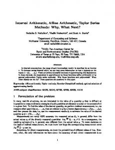
Monotonicity is also exploited in CORA for trigonometric functions as suggested by standard textbooks. However, in none of the checked textbooks [9,12,18,22,24] we have found a detailed description of how all trigonometric functions are implemented. Throughout this subsection, we assume that the arguments of trigonometric functions are in radians. If they are in degree, they can be easily converted to radians upfront. Due to the periodic nature of trigonometric functions, it suffices to only consider intervals whose radius rad([x]) is below a certain threshold. Please note that it is not required to provide implementations for all trigonometric functions, since they depend on each other, e.g. sin([x]) = cos( π2 − [x]). This, however, would require additional operations, such as π2 − [x] in the previous example, which reduces the computational efficiency. For this reason, we suggest the implementations as presented subsequently. We begin with the sin(·) function (see Fig. 2), for which holds sin([x]) = [−1, 1] if x − x ≥ 2π

so that we can focus on the case x − x < 2π. We further simplify the problem by considering only values within the interval [0, 2π[ by using the modulo function from which we obtain y = mod(x, 2π),

y = mod(x, 2π).

(11)

The following proposition helps distinguishing the different cases for obtaining sin([x]): Proposition 1 (Interval bound difference after applying the modulo operator). There only exist two cases for x − x < 2π after applying (11): x − x = y − y (case 1)

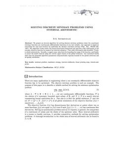
x − x = (y − y) + 2π (case 2) Proof. After applying the modulo operator, we have that y ∈ [0, 2π[ and y ∈ [0, 2π[ so that y − y ∈] − 2π, 2π[. If y − y ∈ [0, 2π[, we obtain case 1 since x − x < 2π and the difference (x − x) − (y − y) can only be a multiple of 2π. The remaining interval is y − y ∈] − 2π, 0[, which results in case 2, since only the addition of 2π ensures x − x = (y − y) + 2π ∈ [0, 2π[. Thus, it suffices to check whether y > y for necessary corrections, since when y ≤ y we know that x − x = y − y. To compute the sin(·) function, we separate the interval [0, 2π[ into three monotonic regions (see Fig. 1) with Rs1 = [0,

π [, 2

π 3π Rs2 = [ , [, 2 2

Rs3 = [

3π , 2π[. 2

If the regions of y and y are equal, we additionally have to check whether y > y holds – this, of course, follows directly when the regions are unequal. Thus, in total, we have 6 combinations of unequal regions and 3 combinations of equal regions, for which we have to check whether y > y. Thus, in total we have 6 + 2 · 3 = 12 cases:

sin([x]) =

  [−1, 1]                         [sin(y), sin(y)]

if

if

         [min(sin(y), sin(y)), 1] if         [−1, max(sin(y), sin(y))] if         [sin(y), sin(y)] if

(x − x ≥ 2π) ∨ (y ∈ Rs1 ∧ y ∈ Rs1 ∧ y (y ∈ Rs1 ∧ y ∈ Rs3 ) ∨ (y ∈ Rs2 ∧ y ∈ Rs2 ∧ y (y ∈ Rs3 ∧ y ∈ Rs3 ∧ y (y ∈ Rs1 ∧ y ∈ Rs1 ∧ y (y ∈ Rs3 ∧ y ∈ Rs1 ) ∨ (y ∈ Rs3 ∧ y ∈ Rs3 ∧ y (y ∈ Rs1 ∧ y ∈ Rs2 ), (y ∈ Rs3 ∧ y ∈ Rs2 ), (y ∈ Rs2 ∧ y ∈ Rs1 ) ∨ (y ∈ Rs2 ∧ y ∈ Rs3 ), (y ∈ Rs2 ∧ y ∈ Rs2 ∧ y

> y) ∨ > y), > y), ≤ y) ∨

(12)

≤ y),

≤ y).

The correctness of each case can be easily checked via visual inspection in Fig. 1; if y > y, the inspection has to be performed as demonstrated in Fig. 2.

1 1

x=y

Rs3

sin(φ)

0.5 0

sin(φ)

0.5

{sin(x)|x ∈ [0, y] ∪ [y, 2π[}

0 -0.5

-0.5

y

x Rs1

-1 0

π/2

Rs2 π

-1 3/2 π

φ [rad]

2π

Figure 1: Regions of sine.

-2 π

-π

0

π

φ [rad]

2π

3π

4π

Figure 2: Movement of infimum and supremum after applying the modulo operator.

For computing the cos(·) function, we only require two monotonic regions (see Fig. 3) with Rc1 = [0, π[,

Rc2 = [π, 2π[.

Thus, in total, we have 2 cases with unequal regions and 4 cases with equal regions, yielding 6 cases:  [−1, 1] if (x − x ≥ 2π) ∨      (y ∈ Rc1 ∧ y ∈ Rc1 ∧ y > y) ∨      (y ∈ Rc2 ∧ y ∈ Rc2 ∧ y > y),  cos([x]) = [cos(y), cos(y)] (13) if (y ∈ Rc2 ∧ y ∈ Rc2 ∧ y ≤ y),    [min(cos(y), cos(y)), 1] if (y ∈ Rc2 ∧ y ∈ Rc1 ),      [−1, max(cos(y), cos(y))] if (y ∈ Rc1 ∧ y ∈ Rc2 ),    if (y ∈ Rc1 ∧ y ∈ Rc1 ∧ y ≤ y). [cos(y), cos(y)]

The tan(·) function has a shorter period of π so that we use slightly different auxiliary angles compared to sin(·) and cos(·): z = mod(x, π),

z = mod(x, π).

For tan(·) we require two monotonic regions (see Fig. 4) with Rt1 = [0, π/2[,

Rt2 = [π/2, π[,

resulting in 6 cases as for cos(·):  ] − ∞, ∞[ if (x − x ≥ π) ∨      (z ∈ Rt1 ∧ z ∈ Rt1 ∧ z     (z ∈ Rt2 ∧ z ∈ Rt2 ∧ z tan([x]) =  (z ∈ Rt1 ∧ z ∈ Rt2 ),      [tan(z), tan(z)] if (z ∈ Rt1 ∧ z ∈ Rt1 ∧ z    (z ∈ Rt2 ∧ z ∈ Rt2 ∧ z

> z) ∨ > z) ∨

(14)

≤ z) ∨ ≤ z).

The cot(·) function is monotonically decreasing in [0, π[ so that we directly obtain ( ] − ∞, ∞[ if (x − x ≥ π) ∨ (z > z), cot([x]) = [cot(z), cot(z)] if (z ≤ z).

(15)

10 1

5

tan(φ)

cos(φ)

0.5 0

0

Rc2

Rc1

-1 0

π/2

π

3/2 π

φ [rad]

-10 0

2π

Figure 3: Regions of cosine.

3

Rt2

Rt1

-5

-0.5

π/2

φ [rad]

π

Figure 4: Regions of tangent.

Vector/Matrix Operations

This section addresses how CORA handles interval vectors and matrices. An interval vector [x] ⊆ Rn , which we denote by a small bold symbol, can be defined as the Cartesian product of n intervals ([x] = [x1 ] × [x2 ] . . . × [xn ]) or as the set bounded by a left vector x ∈ Rn and a right vector x ∈ Rn ([x] = {x|xi ≤ xi ≤ xi , i ∈ {1, . . . , n}}). Analogously, a (m × n)-dimensional interval matrix [X] ⊆ Rm×n , which we denote by a capital bold symbol, can be defined as the Cartesian product of m × n intervals ([X] = [x11 ] × [x12 ] . . . × [x21 ] . . . × [xmn ]) or as the set bounded by a left matrix X ∈ Rm×n and a right matrix X ∈ Rm×n ([X] = {X|xij ≤ xij ≤ xij , i ∈ {1, . . . , m}, j ∈ {1, . . . , n}}). Matrix multiplication and the multiplication of a scalar with a matrix is defined and imple˜ ⊆ Ro×n , [Y] ⊆ Rn×p , and [a] ⊆ R as mented in CORA for [X] ⊆ Ro×n , [X] ([X] [Y])ij =

n X

[X]ik [Y]kj ,

([a] [X])ij = [a] [X]ij .

(16)

k=1

Matrix addition is straightforwardly implemented as ˜ = [X + X, ˜ ˜ X + X]. [X] + [X]

(17)

All unary operations are realized in CORA elementwise as f ([X])ij = f ([X]ij ) Note that we typically compute with larger intervals. For smaller intervals, there exist techniques that directly operate on the center matrix and the radius matrix for computational efficiency [26], but obtain results that are not tight anymore.

4

Implementation in CORA

This section lists the functions realized in CORA. Since CORA is implemented in MATLAB, the function names are chosen such that they overload the built-in MATLAB functions. The

currently implemented functions are listed in Tab. 1 and Tab. 2. The list in Tab. 1 shows which mathematical functions have been realized and Tab. 2 shows all other functions, which are required to specify intervals, arrange them in matrices, access values, perform set operations, display the intervals, among others. Table 1: Methods of the class interval that realize mathematical functions. All functions can be applied to scalars, vectors, or matrices. name abs acos acosh asin asinh atan atanh cos cosh exp log minus mpower mrdivide mtimes plus rdivide sin sinh sqrt tan tanh times uminus uplus

4.1

description returns the absolute value as defined in (10) arccos(·) function as defined in (6) arccosh(·) function as defined in (8) arcsin(·) function as defined in (6) arcsinh(·) function as defined in (8) arctan(·) function as defined in (6) arctanh(·) function as defined in (8) cos(·) function as defined in (13) cosh(·) function as defined in (7) exponential function as defined in (4) natural logarithm function as defined in (5) overloaded ’-’ operator, see (2) overloaded ’ˆ’ operator (power), see (9) overloaded ’/’ operator (division), see (3) overloaded ’*’ operator (multiplication), see (2) for scalars and (16) for matrices overloaded ’+’ operator (addition), see (2) for scalars and (17) for matrices overloads the ’./’ operator: provides elementwise division of two matrices sin(·) function as defined in (12) sinh(·) function as defined in (7) p (·) function as defined in (5) tan(·) function as defined in (14) tanh(·) function as defined in (7) overloaded ’.*’ operator for elementwise multiplication of matrices overloaded ’-’ operator for a single operand overloaded ’+’ operator for single operand

Examples

An interval matrix can be generated by first generating scalar intervals and then assembling them using the same MATLAB syntax as for real-valued variables, or by directly specifying the left and right bounds: 1 2 3 4

a_11 a_12 a_21 a_22

= = = =

interval(-1,1); % generate scalar interval interval(-1,2); % generate scalar interval interval(0.5,1); % generate scalar interval interval(-2,-1); % generate scalar interval

5 6

A_variant1 = [a_11 a_12; a_21 a_22] % generate matrix and display it

7 8 9

A_inf = [-1 -1; 0.5 -2] % specify infimum A_sup = [1 2; 1 -1] % specify supremum

10 11

A_variant2 = interval(A_inf, A_sup) % generate matrix and display it

12 13

firstElement = A_variant2(1,1) % obtain and display first element

Table 2: Methods of the class interval that do not realize mathematical functions. All functions can be applied to scalars, vectors, or matrices. name and display horzcat infimum interval isempty isscalar length mid rad size subsasgn subsref supremum transpose vertcat

14 15

description returns the intersection as defined in (1) displays the values of the interval object in the MATLAB workspace overloads the operator for horizontal concatenation, e.g. a = [b,c,d] returns the infimum of an interval constructor of the interval class returns 1 if interval is empty and 0 otherwise returns 1 if interval is scalar and 0 otherwise overloads the operator that returns the length of the longest array dimension returns the center of an interval returns the radius of an interval overloads the operator that returns the size of the object, i.e., length of an array in each dimension overloads the operator that assigns elements of an interval matrix I, e.g. I(1,2)=value, where the element of the first row and second column is set overloads the operator that selects elements of an interval matrix I, e.g. value=I(1,2), where the element of the first row and second column is read returns the supremum of an interval overloads the ’.’ ’ operator to compute the transpose of an interval matrix overloads the operator for vertical concatenation, e.g. a = [b;c;d]

firstRow = A_variant2(1,:) % obtain and display first row secondColumn = A_variant2(:,2) % obtain and display second column

This produces the workspace output A_variant1 = [-1.00000,1.00000] [-1.00000,2.00000] [0.50000,1.00000] [-2.00000,-1.00000] A_variant2 = [-1.00000,1.00000] [-1.00000,2.00000] [0.50000,1.00000] [-2.00000,-1.00000] firstElement = [-1.00000,1.00000] firstRow = [-1.00000,1.00000] [-1.00000,2.00000] secondColumn = [-1.00000,2.00000] [-2.00000,-1.00000]

Mathematical functions are evaluated using the MATLAB syntax as for real-valued variables: 1 2 3

A_inf = [-1 -1; 0.5 -2]; % specify infimum A_sup = [1 2; 1 -1]; % specify supremum A = interval(A_inf, A_sup); % generate matrix

4 5 6

B_inf = [0 -1; 0 1]; % specify infimum B_sup = [1 3; 0.5 1.2]; % specify supremum

7

B = interval(B_inf, B_sup); % generate matrix

8 9 10 11 12 13 14 15 16 17

A+B % addition A*B % multiplication A.*B % pointwise multiplication A/interval(1,2) % division A./B % pointwise division Aˆ3 % power function sin(A) % sine function sin(A(1,1)) + A(1,1)ˆ2 - A(1,1)*B(1,1) % scalar combination of functions sin(A) + Aˆ2 - A*B % matrix combination of functions

This produces the workspace output

A+B = [-1.00000,2.00000] [-2.00000,5.00000] [0.50000,1.50000] [-1.00000,0.20000] A*B = [-1.50000,2.00000] [-4.20000,5.40000] [-1.00000,1.00000] [-3.40000,2.00000] A.*B = [-1.00000,1.00000] [-3.00000,6.00000] [0.00000,0.50000] [-2.40000,-1.00000] A/interval(1,2) = [-1.00000,1.00000] [-1.00000,2.00000] [0.25000,1.00000] [-2.00000,-0.50000] A./B = [-Inf,Inf] [-Inf,Inf] [1.00000,Inf] [-2.00000,-0.83333] A^3 = [-9.00000,7.00000] [-12.00000,18.00000] [-3.00000,9.00000] [-18.00000,3.00000] sin(A) = [-0.84147,0.84147] [-0.84147,1.00000] [0.47943,0.84147] [-1.00000,-0.84147] sin(A(1,1)) + A(1,1)^2 - A(1,1)*B(1,1) = [-1.84147,2.84147] sin(A) + A^2 - A*B = [-4.84147,5.34147] [-12.24147,9.10930] [-3.52057,2.34147] [-2.90930,8.55853]

4.2

Comparison with INTLAB

In this subsection, we compare the speed and accuracy of our implementation with INTLAB. Please note that we do not compare the results with b4m [31] since this tool no longer runs on current MATLAB versions. Since INTLAB considers rounding errors of floating-point numbers, the results of INTLAB are slightly larger intervals due to outwards rounding. As mentioned in the introduction, the first version of interval arithmetic realized in CORA does not consider floating-point errors, since they are also not considered in other computations of CORA. The main purpose of CORA is to prototypically realize algorithms for reachable set computations. Once an algorithm is mature, one should consider rounding errors when aiming for a commercial tool. Since we neglect floating-point errors, our implementation is faster for almost all functions compared to INTLAB as shown in Tab. 3. The computation times have been averaged from 104 runs for each function and have been carried out on an Intel Core i5-3230M processor running at 2.60GHz. Please note that this is an old processor and computation times have been observed to be more than 100 times faster on a modern processor. Let us introduce the left and right bound of the j th out of N = 104 evaluations of a particular function in CORA as xC,j and xC,j . Likewise, the bound of the j th evaluation using INTLAB is denoted by xI,j and xI,j . The maximum relative error over all runs is defined as ǫ = max(µ1 , . . . , µN ),

µj =

max(|xC,j − xI,j |, |xC,j − xI,j |) . xC,j − xC,j

(18)

We have used the same 104 runs for each function as for measuring the average computation time. We introduce the random variables U and U∆ , which are uniformly distributed within an interval. The interval for U is [u, u] and the one for U∆ is [u∆ , u∆ ]. We construct the following random input intervals for unary operations: [U, U + U∆ ]. For binary operations, this random interval is computed twice. For our implementation, we have used the standard precision of MATLAB floating point numbers, which is the double-precision data type according to the IEEE 754 standard. The bound of the random variables vary depending on the tested function and are listed in Tab. 3. The results of the evaluation in Tab. 3 show that the maximum relative error ǫ over all runs is marginal compared to the range of intervals xC,j − xC,j .

5

Conclusions

This paper has three main contributions. First, we present how we integrate interval arithmetic into CORA and list all implemented methods. Currently, we provide the only freely available MATLAB implementation of interval arithmetic running under the latest MATLAB versions. Second, we compare our implementation to INTLAB; the main result of our comparison is that our tool obtains results faster, but does not consider floating-point errors. These, however, are also not yet considered in the other methods provided by CORA, mainly since the tool is designed for prototypically testing different approaches for reachability analysis. The resulting error from neglecting floating-point arithmetic is marginal for the tested functions. Finally, we provide all required formulas for evaluating the range of functions – all previous works referenced in here do not provide such an exhaustive list, but only point out that monotonicity should be considered when evaluating functions. We admit that the evaluations of functions are not difficult, but especially when considering cases where the input interval is not within the

Table 3: Comparison with INTLAB. avg. comp. time [s] function error ǫ; see (18) abs 0 acos 4.711 · 10−12 acosh 8.208 · 10−13 asin 1.948 · 10−12 asinh 2.304 · 10−12 atan 5.915 · 10−11 atanh 4.801 · 10−12 cos 8.515 · 10−13 cosh 1.865 · 10−14 exp 2.627 · 10−14 log 2.028 · 10−11 minus 7.583 · 10−15 3 mpower (() ) 1.873 · 10−12 mrdivide 4.656 · 10−15 mtimes 4.053 · 10−15 plus 3.327 · 10−15 rdivide 4.896 · 10−15 sin 3.139 · 10−13 sinh 1.902 · 10−12 sqrt 1.407 · 10−12 tan 5.627 · 10−12 tanh 1.418 · 10−12 times 9.434 · 10−15 uminus 0 uplus 0

INTLAB 7.388 · 10−5 4.881 · 10−4 5.433 · 10−4 4.318 · 10−4 5.196 · 10−4 3.179 · 10−4 4.711 · 10−4 4.857 · 10−4 3.971 · 10−4 2.262 · 10−4 3.090 · 10−4 9.846 · 10−5 2.993 · 10−4 2.300 · 10−4 1.817 · 10−4 9.453 · 10−5 2.056 · 10−4 4.093 · 10−4 3.224 · 10−4 1.524 · 10−4 5.371 · 10−4 2.432 · 10−4 1.828 · 10−4 1.880 · 10−5 1.078 · 10−5

input intervals

CORA u 8.503 · 10−5 −100 1.346 · 10−4 −1 1.279 · 10−4 1 1.282 · 10−4 −1 1.131 · 10−4 −100 1.081 · 10−4 −100 1.271 · 10−4 −1 1.086 · 10−4 −100 1.203 · 10−4 −100 6.840 · 10−5 −100 1.127 · 10−4 0 8.425 · 10−5 −100 1.550 · 10−4 0 3.449 · 10−4 −100 1.208 · 10−4 −100 5.625 · 10−5 −100 2.735 · 10−4 −100 9.839 · 10−5 −100 1.044 · 10−4 −100 1.163 · 10−4 0 1.267 · 10−4 − π2 + 0.1 1.050 · 10−4 −1 1.257 · 10−4 −100 3.452 · 10−5 −100 1.631 · 10−5 −100

u u∆ 100 0 0 0 10 0 0 0 100 0 100 0 0 0 100 0 100 0 100 0 100 0 100 0 100 0 100 0 100 0 100 0 100 0 100 0 100 0 100 0 0 0 1 0 100 0 100 0 100 0

u∆ 100 1 10 1 100 100 1 100 100 100 100 100 100 100 100 100 100 100 100 100 π 2 − 0.1 1 100 100 100

domain of a function, we believe that a complete documentation of the implemented algorithms is beneficial.

Acknowledgment The authors gratefully acknowledge financial support by the European Commission project UnCoVerCPS under grant number 643921.

References [1] IEEE standard for interval arithmetic. IEEE Std 1788-2015, pages 1–97, June 2015. [2] A.Eggers, N. Ramdani, N. S. Nedialkov, and M. Fr¨ anzle. Improving the sat modulo ode approach to hybrid systems analysis by combining different enclosure methods. Software & Systems Modeling, 14(1):121–148, 2012.

[3] G. Alefeld and G. Mayer. Interval analysis: Theory and applications. Computational and Applied Mathematics, 121:421–464, 2000. [4] M. Althoff. An introduction to CORA 2015. In Proc. of the Workshop on Applied Verification for Continuous and Hybrid Systems, pages 120–151, 2015. [5] E. Asarin, T. Dang, G. Frehse, A. Girard, C. Le Guernic, and O. Maler. Recent progress in continuous and hybrid reachability analysis. In Proc. of the 2006 IEEE Conference on Computer Aided Control Systems Design, pages 1582–1587, 2006. ´ [6] X. Chen, E. Abrah´ am, and S. Sankaranarayanan. Flow*: An analyzer for non-linear hybrid systems. In Proc. of Computer-Aided Verification, LNCS 8044, pages 258–263. Springer, 2013. [7] J. S. Ely. The VPI software package for variable precision interval arithmetic. Interval Computations, 2:135–153, 1993. [8] D. Goldberg. What every computer scientist should know about floating point arithmetic. ACM Computing Surveys, 23(1):5–48, 1991. [9] R. Hammer, M. Hocks, U. Kulisch, and D. Ratz. C++ Toolbox for Verified Computing I. Springer, 1995. [10] M. Herceg, M. Kvasnica, C.N. Jones, and M. Morari. Multi-Parametric Toolbox 3.0. In Proc. of the European Control Conference, pages 502–510, Z¨ urich, Switzerland, July 17–19 2013. http://control.ee.ethz.ch/~ mpt. [11] F. Immler. Tool presentation: Isabelle/HOL for reachability analysis of continuous systems. In Proc. of the 2nd Workshop on Applied Verification for Continuous and Hybrid Systems., pages 180–187, 2015. [12] L. Jaulin, M. Kieffer, and O. Didrit. Applied Interval Analysis. Springer, 2006. [13] J. C. Jensen, D. H. Chang, and E. A. Lee. A model-based design methodology for cyber-physical systems. In Proc. of the 7th International Wireless Communications and Mobile Computing Conference, pages 1666–1671, 2011. [14] R. B. Kearfott. Algorithm 763: INTERVAL ARITHMETIC: A Fortran 90 module for an interval data type. ACM Transactions on Mathematical Software, 22(4):385–392, 1996. [15] R. B. Kearfott, M. Dawande, K. Du, and C. Hu. Algorithm 737: INTLIB: A portable Fortran 77 interval standard-function library. ACM Transactions on Mathematical Software, 20(4):447–459, 1994. [16] O. Kn¨ uppel. PROFIL/BIAS V 2.0. Technical report, Technische Universit¨ at Hamburg-Harburg, 1999. [17] S. Kong, S. Gao, W. Chen, and E. Clarke. dReach: δ-reachability analysis for hybrid systems. In Proc. of Tools and Algorithms for the Construction and Analysis of Systems, 200-205, pages 200–205, 2015. [18] U. W. Kulisch and W. L. Miranker. Computer Arithmetic in Theory and Practice. Academic Press, 1981. [19] E. A. Lee. CPS foundations. In Proc. of the 47th Design Automation Conference, pages 737–742, 2010. [20] V. Lef`evre, J.-M. Muller, and A. Tisserand. Toward correctly rounded transcendentals. IEEE Transactions on Computers, 47(11):1235–1243, 1998. [21] S. Mitra, T. Wongpiromsarn, and R. M. Murray. Verifying cyber-physical interactions in safetycritical systems. IEEE Security and Privacy, 11(4):28–37, 2013. [22] R. E. Moore, R. B. Kearfott, and M. J. Cloud. Introduction to Interval Analysis. Society for Industrial and Applied Mathematics, 2009. [23] R. Poovendran. Cyber-physical systems: Close encounters between two parallel worlds. Proceedings of the IEEE, 98(8):1363–1366, 2010. [24] H. Ratschek and J. Rokne. Computer Methods for the Range of Functions. Halsted Pr, 1984. [25] S. M. Rump. Developments in Reliable Computing, chapter INTLAB - INTerval LABoratory,

pages 77–104. Kluwer Academic Publishers, 1999. [26] S. M. Rump. Fast and parallel interval arithmetic. BIT Numerical Mathematics, 39(3):534–554, 1999. ´ [27] S. Schupp, E. Abrah´ am, X. Chen, I. Ben Makhlouf, G. Frehse, S. Sankaranarayanan, and S. Kowalewski. Current challenges in the verification of hybrid systems. In Proc. of the Fifth Workshop on Design, Modeling and Evaluation of Cyber Physical Systems, pages 8–24, 2015. [28] Sun Microsystems, Inc., 901 San Antonio Road Palo Alto, CA 94303 U.S.A. 650-960-1300. C++ Interval Arithmetic Programming Reference, 2001. [29] J. Sztipanovits, S. Ying, I. Cohen, D. Corman, J. Davis, H. Khurana, P. J. Mosterman, V. Prasad, and L. Stormo. Strategic R&D opportunities for 21st century cyber-physical systems. Technical report, National Institute of Standards and Technology (NIST), 2013. [30] W. Wolf. Cyber-physical systems. Computer, 42(3):88–89, 2009. [31] J. Zemke. b4m — A free interval arithmetic toolbox for Matlab based on BIAS. Technical report, Arbeitsbereich Technische Informatik III 4-04, Technische Universit¨ at Hamburg-Harburg, 1999.