Implementation of meta-heuristic algorithms for supplier selection and

Jurnal UMP Social Sciences and Technology Management

Vol. 3, Issue. 3,2015

Implementation of meta-heuristic algorithms for supplier selection and evaluation and multi product order allocation Ali Nazeri, Department of Industrial Engineering, Technology Development Institute (ACECR), Tehran, Iran

Morteza Khakzar Bafruei Department of Industrial Engineering, Technology Development Institute (ACECR), Tehran, Iran. Corresponding Author [email protected]

Abstract In this article, a multi-objective mathematical programming model is presented to consider quantitative and qualitative factors and risk to choose appropriate suppliers and allocate the optimal order quantity to them. The primary evaluation of suppliers is done by use of an analytical hierarchy process and utilization of the results for multiobjective modeling. The designed model is solved by NSGA-II and MOPSO algorithms. A T-test is used to compare both algorithms’ performance. On the basis of analytical results, there is no difference in using either one for problem solving. Finally, the problem is solved by NSGA-II, an obtained Pareto solution set is ranked by the TOPSIS algorithm, and then the best possible solution is chosen. Key words: Supplier Selection and Evaluation, MOPSO Algorithm, NSGA-II Algorithm, Order allocation, multi-objective programming Introduction A working definition of supply chain management (SCM) includes network optimization comprised of procurement, manufacturing, warehousing, and transportation systems. A series of trade-offs is required of management based on business costs. SCM is generally considered as an effective means to help companies reduce costs, improve responsiveness, and increase competitiveness. Designing an integrated system which would involve the entire supply chain network is required in order to remain competitive in the global marketplace, thus the increased focus on planning and management of the flow of materials from suppliers to end users. (Kumar et al, 2004).Ideally, flexibility and a high level of responsiveness are required of suppliers in meeting the orders of end users, with the result that the proper selection of supplies is critical. In managing a supply network, almost all subsequent decisions are impacted by supplier evaluation and selection. Purchasing costs are reduced, competitiveness is improved, end user satisfaction is increased, as waste is eliminated and lead time at the different stages of the network is reduced. Different tangible and intangible variables including price, quality, performance, technical capability and delivery are components of MCDM, or multiple-criteria decisionmaking problems. (Kumar et al, 2004).There are two main types of supplier selection. The first is single sourcing, where one supplier can satisfy all the entire buyer’s needs, such that the buyer must make only one decision, which is the selection of the best supplier. In the second type, which is more common,

566

Jurnal UMP Social Sciences and Technology Management

Vol. 3, Issue. 3,2015

more than one supplier is needed as one supplier cannot meet all of the buyers’ demands. This is known as multiple sourcing. Thus, to remain competitive, companies must select not only the best suppliers but must also decide how much quantity should be allocated among them (Alyanak, Armaneri, 2009). Of the two, multiple sourcing goes farther in ensuring timely delivery and order flexibility as there is great diversity in the total orders of the firm. (Ghodsypour, O’Brien, 1998) (Jolai, et al, 2011) .Many different individual and integrated approaches have been generated in terms of supplier selection. A number of integrated approaches for sourcing of multiple supplier have been reviewed by (Ho et al, 2010) who concluded that the integrated AHP-GP approach is most popular, due mainly to its simplicity, ease of use, and flexibility (Kannan, Vinay, 2008) (Borade, et al, 2013). MCDM, multi criteria decision making and MODM, multi-objective decision making, both use Goal Programming on a wide basis due to its simplicity and flexibility. Relatively large numbers of decision variables, resource constraints, and objectives can be handled by goal programming (Jolai, et al, 2011)( Dubey, et al, 2012), which is a branch of multi-objective optimization in which linear programming is extended in order to deal with multiple, normally conflicting objectives (Jolai, et al, 2011)( Chang, et al, 2011)( Lee, et al, 2009).A systematic literature review was provided by (Chai et al, 2013). This review was based on 123 journal articles published from 2008 to 2012 on the application of decision making (DM) techniques for supplier selection. AHP followed by linear programming (LP) and Technique for Order of Preference by Similarity to Ideal Solution (TOPSIS) were shown to be the most frequently used techniques. A literature review conducted by (Wu, Barnes, 2011) based on articles published between 2001 and 2010 based on supply partner decision-making drew the conclusion that the most well-known approaches for supplier selection problem are the models that include mathematical programming, AHP/ANP, or fuzzy set approach.In addition, many other evolutionary algorithms for solving multi-objective optimization problems such as niched Pareto genetic algorithm 2 (Erickson, et al, 2001), non-dominated sorting genetic algorithm II (NSGA-II) (Deb, et al, 2002), strength Pareto evolutionary algorithm 2 (Zitzler, et al,2000), Pareto-archived evolution strategy (Knowles, Corne, 2000) have been proposed. This research uses a multi-objective non-linear programming model designed with consideration of qualitative and quantitative factors to determine the optimal number of orders in a multi-product situation. NSGA-II and MOPSO were adopted to solve the optimization problem. NSGA-II and MOPSO have been used due to their proven ability to solve combinatorial optimization problems when compared to traditional optimization techniques (Goldberg, 1998), (Steiner, Hruschka, 2002). In addition, this research acknowledges that some objective functions are non-linear and cannot be solved by deterministic solution methods. Problem Statement and Proposed Model Let us assume that in a given period, a buyer can purchase m products from n supplier and has a constant demand. The set of suppliers on the basis of some certain criteria, such as quality, services, delivery, maintenance, and so on, have been pre-selected, and the type of orders is multi-product. Also, let us suppose that the capacity of each supplier is limited, and the value of order to supplier must be equal or greater to supplier capacity. This state is a close fit to a real business scenario. This article aims to determine the order value to assign each supplier and to minimize supply risk, delay time, reduce the percentage of defective products and cost while maximizing supplier capacity.

765

Implementation of meta-heuristic…

www.jsstm-ump.org

In this section, a MONLP model is presented to allocate orders. The MONLP objective function includes a set of goals that are in conflict with each other and must be fulfilled simultaneously. It is difficult to provide the optimal solution for MONLP. The aim of MONLP methods is finding a preferred answer among the most effective points (Chang, et al, 2011). In this paper, a MONLP model is presented to solve suppliers’ selection problem which is the main purpose of the allocation order with regard to limitations, such as supplier capacity, defective products, delivery time, the risk of failure, and supply risk. The following assumptions were used in the formulation of MONLP model: a) It is possible to purchase multi products from each supplier. b) Product shortage is not allowed for suppliers. c) Demand is deterministic. The following Symbols were used in the formulation of model: Parameters m: Number of suppliers n: Number of products Dj: Demand for product j Xij: The amount of product j assigned to supplier i Cij: The capacity of supplier i to supply product j Wi: Weight of importance given to supplier i(AHP output) Pij: The price of product j purchased from supplier i Qj: The maximum acceptable rate of defect for product j qij: The average defect of product j purchased from supplier i tij: The rate delay of delivery of product j purchased from supplier i rij:: The rate of risk of product j purchased from supplier i Ci: The cost of risk of supplier i CR: The maximum cost of risk B: The maximum budget for purchase M: A large number 1.1.1.

Objective functions:

(1) Assign the maximum amount of order to appropriate supplier, MAX Z1= ∑

∑

(2)Minimize the cost of purchases, ∑

MIN Z2=∑

(3)Minimize the rate of delay, MIN Z3=

∑

∑

∑

∑

(4)Minimize the rate of defects, MIN Z4 =

∑

∑

∑

∑

(5)Minimize the rate of supply risk, MIN Z5= 765

∑ ∑

∑ ∑

Jurnal UMP Social Sciences and Technology Management

Vol. 3, Issue. 3,2015

Constraints: For modeling problems, in both first constraints, variable supply j is allocated to supplier i, then

=1 unless

must be determined in such a way if good

= 0. Constraint 2 represents the cost to ensure

compliance with maximum financial risk for the company. Constraint 3 shows the budget for the purchase that should be less than B. Constraint 4 demonstrates the total demand for product j which must be supplied by all suppliers. Constraint 5 guarantees the maximum acceptable percentage of defective items, and finally, Constraint 6 explains the order amount assigned to each supplier which must be equal to or less than the supply capacity. ∑

1)

{

2)

∑

3)

∑

4)

∑

5)

∑

∑ ∑

6) In this research, combination of AHP and MONLP methods is used to solve supplier selection and order allocation problems. At first, the AHP method was used to calculate the relative weight of the supplier selection criteria, then the selected criteria were ranked by AHP, and finally weighting of criteria and rank of supplier is given to the MONLP model. The model, in terms of constraints, specifies the optimum number of suppliers and amount of optimal order for each supplier. MOPSO and NSGA-II algorithms are considered to solve the model. The aforementioned model is solved by both algorithms using 9 numerical examples and then compared with each other by use of criteria. In the next section, comparable indicators are described. Comparison Indexes Two main metric categories for the evaluation of multi-objective heuristic algorithms exist: 1) convergence metrics and 2) scattering metrics. Comparison is made in this paper using seven Indexes that are combinations of two main metric categories. The first category's criteria include Pareto, Mean Ideal Distance (MID), and Coverage criteria set (NH), and the second category's criteria consist of Spacing Criteria, diversity and Maximum Spread. In addition, Time criteria for fiscal necessity are considered. Number of Pareto solution (NOS) criteria The quantity of NOS criteria demonstrates the Number of Pareto optimal solutions that can be produced by each algorithm. (Zitzler, et al, 2000) Mean distance from the Ideal answer This criterion is used to calculate the mean Pareto answers distance from the origin coordinates. In Equation 1 it is distinctive; the smallest criterion provides the most efficient algorithm. M ID 

1 NOS

NOS

 i 1

m

ci w h ere ci 



f

2 ji

j 1

Since one of the aims in multi objective discussion based on Pareto approach is to have closer boundaries to the origin coordinates, this criteria calculates the distance of borders to the best amount 765

Implementation of meta-heuristic…

www.jsstm-ump.org

of Swarm.n is the number of Pareto answers where the mean distance from Ideal point( ) is obtained as mentioned in the Index.( Zitzler, et al, 1998). Set Coverage Metric (NH) he ratio of B answers that are dominated by A answers. It is calculated through the use of Equation 2. (

)

{

}

In this Equation, if the amount of ( (

) equals 1, all B members are dominated by A members and if

)=0, no B members are dominated. Therefore, when (

) is greater than (

), in this criteria

set A is better than Set B. (C.A. Coello Coello, et al, 2002) Spacing Criteria This criterion has been presented by Schott 1995, and is calculated as the relative distance of continuous answers by use of Equation 3. (Schott, 1995) √

̅)

∑(

⏟

where

,̅

∑

∑

The measured distance is equal to the minimum sum of the absolute value of the difference in the values of objective functions between the ith answer and the answer located in final non-dominated set. It should be mentioned that there is a difference between spacing criteria and minimum distance among answer criteria. This criterion measures the deviation of different values of

. Whenever the answers set beside each

other, then the value of s is small. Therefore, the best algorithm has a final non-dominated answer with little spacing quantity. Diversification Metric (DM) This Index calculates diversity among all categories of non-dominated answers, and the formula is as follows: √∑

(|

|)

| is a direct distance between non-dominated solution

Where|

and

. Whichever criterion is

greater indicates fewer of the same answers, and variety among answers is greater. A large quantity of these criteria is more desirable for this purpose. (Zitzler, Thiele, 1998). Maximum spread criteria This criterion as presented by Zitzler 1999, measures the diameter length of the cubic space by the final values for each objective function. Non-dominated solutions were used. Equation 1 shows the procedure of calculating the criterion. (Zitzler, 1999). m

D 

 j 1

755

(m ax fi i

j

 m in f i ) j

i

2

Jurnal UMP Social Sciences and Technology Management

Vol. 3, Issue. 3,2015

In multi objective state, this criterion is equal to the distance between two boundary responses of objective area. The maximum length for this criterion is the most effective. Whatever this criteria is greater, is better. Time criteria Time of running the algorithm is considered as a quality assessment criterion. Numerical Examples In this paper, nine different problems in different sizes have been considered. The number of products varied from 3 to 8, and the number of suppliers varied from 5 to 50. Additional details are shown in the following tables. Table1 .The parameters used for NSGA-II Number of Initial Swarm Combination Repeats Rate 150 30 0.7 150 50 0.6 100 50 0.6 Table 2.The parameters used for MOPSO

Problem size Small (sample1,2,3) Medium(sample4,5,6) Large(sample7,8,9) Problem size

Number Repeats

Small (sample1,2,3) Medium(sample4,5,6) Large(sample7,8,9)

150 100 100

of

Initial Swarm

50 40 30

The Best Neighborhood effective Rate 1.1 2.8 1.1

Mutation Rate 0.3 0.2 0.2 The Best particle effective Rate 1.1 1.1 2

Before describing the results for each of these algorithms, it should be mentioned that for these three indexes, Non-dominated solutions (NOS), Diversity and Spread, higher amounts are desirable. In addition, some of objective functions are maximization. First, they should be multiplied by a negative to achieve minimization. For the other criterion, the minimum amount is desirable. The values of mentioned criteria for sample issues are described below: Table 3 Test Problem Number 1

NSGA II SPREAD

Diversity

MOPSO SPREAD

SPACING

SPACING

Diversity

491620

190360

3450.3

476220

127750

2505.70

2

434840

108340

3654.6

478290

307330

622.9089

3

637190

314250

4112.7

651740

275010

2766.50

4

1116200

169310

3336

742630

280980

3530.10

5

1136700

135190

4125.4

1044200

207600

1952.20

6

866720

344690

2094.2

1079300

294580

2058.40

7

889600

155030

4188.3

835890

341100

1294.10

8

1530700

228070

2175.1

1432300

214830

1117.6

9

1346100

655990

1117.6

1364600

227100

171.4617

755

Implementation of meta-heuristic…

www.jsstm-ump.org

Table 4 Test Problem Number

NSGA II

MOPSO

MID

NOP

NH

Time

MID

NOP

NH

Time

1

45196000

182

0.0385

4.3666

47151000

150

0.4400

5.3091

2

48686000

150

0.3933

5.2221

49134000

159

0.1761

3.4291

3

51646000

124

0.3145

3.2001

51279000

121

0.2893

2.8462

4

87064000

111

0.0991

2.8160

84833000

107

0.4393

2.7753

5

86990000

150

0.6000

4.5723

88145000

151

0.0662

3.5201

6

103050000

116

0.1897

2.8396

100020000

106

0.5943

3.0226

7

101230000

139

0.6187

3.8840

104200000

182.

0.0330

5.6249

8

118860000

156

0.1154

11.2943

121620000

150

0.1467

4.3839

9

137290000

190

0.0789

13.9236

135520000

150

0.4333

5.4643

150000000 100000000 NSGA II 50000000

MOPSO

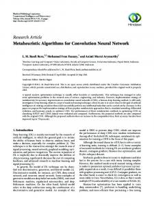
0 1 2 3 4 5 6 7 8 9 Chart1.A comparison of two algorithms with MID metric 200.0000 150.0000 NSGA II

100.0000

MOPSO

50.0000 0.0000 1 2 3 4 5 6 7 8 9

Chart2.A comparison of two algorithms with NOP metric

752

Jurnal UMP Social Sciences and Technology Management

Vol. 3, Issue. 3,2015

0.7000 0.6000 0.5000 0.4000

NSGA II

0.3000

MOPSO

0.2000 0.1000 0.0000

1 2 3 4 5 6 7 8 9 Chart3.A comparison of two algorithms with NH metric 15.0000

10.0000 NSGA II 5.0000

MOPSO

0.0000

1 2 3 4 5 6 7 8 9 Chart4.A comparison of two algorithms with TIME metric 2000000.0000 1500000.0000 NSGA II

1000000.0000

MOPSO 500000.0000 0.0000 1 2 3 4 5 6 7 8 9 Chart5.A comparison of two algorithms with SPREAD metric

753

Implementation of meta-heuristic…

www.jsstm-ump.org

700000.0000 600000.0000 500000.0000 400000.0000

NSGA II

300000.0000

MOPSO

200000.0000 100000.0000 0.0000 1 2 3 4 5 6 7 8 9

Chart6.A comparison of two algorithms with SPACING metric 5000.0000 4000.0000 3000.0000 2000.0000 1000.0000 0.0000 1

2

3

4

NSGA II

5

6

7

8

9

MOPSO

Chart7.A comparison of two algorithms with DIVERSITY metric Performance analysis of both algorithms To evaluate which algorithm is more desirable, we need to use statistical analysis. In this survey we have used the technique of hypothesis testing; thus, we have considered null hypothesis equality means of assessment criteria at both algorithms with 95% confidence levels.If the P-value obtained is less than 0.05, the null hypothesis is rejected, and we conclude there are significant differences between the criteria for evaluating the performance of the algorithms and vice versa. Statistical properties of the seven criteria for both algorithms are shown in Table 5. Table 5.Statistical properties of the seven criteria for both algorithms SECTION N Mean Std. Deviation MID NOH NH TIME SPREAD SPACING DIVERSITY

754

Std. Error Mean

NSGAII MOPSO NSGAII

9 9 9

86668000 86878000 146.4444

32535929.385 32252392.849 27.43224

10845309.7952 10750797.6164 9.14408

MOPSO NSGAII MOPSO NSGAII MOPSO NSGAII

9 9 9 9 9 9

141.7778 .2720 .2909 5.7910 4.0417 938852.2

25.30700 .22285 0.19607 4.00272 1.17114 377393.10373

8.43567 .07428 0.06536 1.33424 0.39038 125797.70124

MOPSO NSGAII MOPSO NSGAII MOPSO

9 9 9 9 9

900574.4 255692.2 252920 3139.355 1779.885

353566.27017 169723.10146 64793.90365 1091.46886 1076.50824

117855.42339 56574.36715 21597.96788 363.82295 358.83608

Jurnal UMP Social Sciences and Technology Management

Vol. 3, Issue. 3,2015

In column 6 of Table 6, the P-value is presented, and for each criterion two amounts of P-value are evaluated. The first one is used when standard deviation for both populations is equal; otherwise we must use the second P-value. As shown in Table 2, there is no significant difference between 6 criteria as both algorithms have the same performance, but the difference is in variety criteria which is negligible. Thus, it makes no difference which algorithm is used. Table 6.Equality Average hypothesis testing of seven criteria

Selecting the best Pareto answer As analyzed, no one algorithm is preferable to another on the basis of defined criteria. Now, we solve the same problem by a numerical example using 10 suppliers, 3 products and the NSGA-II algorithm and check the result. The parameters used to solve the example are described below: Table 7-Probability distribution functions for parameters Parameter U(a,b) U(0.3,1) U(0.02,.07) U(150,350) U(.1,.15) U(.1,.6) U(55000,75000) U(1500,3500) U(.07,.09) U(40000,50000)

575

Implementation of meta-heuristic…

www.jsstm-ump.org

After the algorithm execution, 150 answers were found and ranked by the TOPSIS method. Objective functions are considered as TOPSIS method criteria, and their weight is obtained by AHP according to Table 8. Criteria Weight

Objective1 0.02

Table 8 Objective 2 Objective 3 0.06 0.12

Objective 4 0.40

Objective 5 0.40

According to TOPSIS ranking, Pareto Answer 4 is selected as the best answer with desirable coefficients 0.647, followed by 98 and Pareto Answer 6 with desirable coefficients 0.637 and 0.635, respectively. Pareto Answer 4 is as follows, based on 10 initial suppliers, No.4, 5, 6, 8 have been selected (table 9). Supplier

Table 9 1st Product 2nd Product

3rd Product

Supplier 4

0

0

36710

Supplier 5

38165

46440

34290

Supplier 6

28835

0

0

Supplier 8

0

23560

0

The objective function values are as follows: st 1 objective function: 1683060 nd 2 objective function: 0.43 rd 3 objective function: 0.92 Th 4 objective function: 49623140 th 5 objective function: 0.2 Conclusion and Suggestions for future research This paper presents a model of supplier selection and Multi-Objective Order assignment for supply chain outsourcing risk management. Some of the suppliers’ selection of quantitative and qualitative factors and risk are considered. This model is an integrated model and is effecting to utilize by firms. The presented model is coded and solved by MATLAB software, NSGA-II, and MOPSO algorithms. The answers obtained by each algorithm were compared to the mean comparison test, and according to the defined criteria, NSGA-II was found to be an efficient algorithm. Suggestions for future research include adding other objective functions in accordance with organizational conditions, consideration of additional variables, converting the model to fuzzy mode, changing the constraints and solving the model by other meta-heuristic algorithms, working on the set of parameters or adding delivery to the problem and delivery time.

576

Jurnal UMP Social Sciences and Technology Management

Vol. 3, Issue. 3,2015

References 1. Alyanak, G. & Armaneri, O. (2009). An integrated supplier selection and order allocation approach in a battery company. Makine Mühendisleri Odasi 19 (4), 2-19. 2. Borade, A.B., Govindan, K. & Bansod, S.V., (2013). Analytical hierarchy process based framework for VMI adoption. International Journal of Production Research 51 (4), 963-978. 3. Chai, J., Liu, J.N.K. & Ngai, E.W.T., (2013). Application of decision-making techniques in supplier selection: a systematic review of literature. Expert Systems with Applications 40, 3872-3885. 4. Chang, B., Chang, C.W. & Wuc, C.H., (2011). Fuzzy DEMATEL method for developing supplier selection criteria, Expert Systems with Applications 38, 1850-1858. 5. Coello Coello, C.A. Van Veldhuizen D.A. & Lamont, G.B. (2002). Evaluationary Algorithm for solving Multi-objective problems, Kluwer Academic Publishers, New York, first edition, May, ISBN, 0- 7062-6364-7, and 4004. 6. Deb, K., Pratap, A. & Agarwal, S. & Meyarivan, T. (2002). A fast and elitist multiobjective genetic algorithm: NSGA-II. IEEE Transactions on Evolutionary Computation, 6(2), 182–197. 7. Dubey, O.P., Dwivedi, R.K. & Singh, S.N. (2012). Goal programming: a survey (1960-2000). IUP Journal of Operations Management 14 (2), 29-53. 8. Erickson, M., Mayer, A. & Horn, J. (2001). The Niched Pareto genetic algorithm 2 applied to the design of groundwater remediation systems. Proceedings, evolutionary multi-criterion optimization (pp. 681–695). Springer-Verlag. 9. Ghodsypour, S.H. & O’Brien, C. (1998). A decision support system for supplier selection using an integrated analytic hierarchy process and linear programming. International Journal of Production Economics 56-57, 199-212. 10.Goldberg, D.E., (1998). Genetic Algorithms in Search, Optimisation, and Machine Learning. Addison-Wesley, New York. 11. Ho, W., Xu, X. & Dey, P.K. (2010). Multi-criteria decision making approaches for supplier evaluation and selection: a literature review. European Journal of Operational Research 202, 16-24. 12. Jolai, F., Yazdian, S.A. & Shahanaghi, K. & Azari Khojasteh, M. (2011). Integrating fuzzy TOPSIS and multi-period goal programming for purchasing multiple products from multiple suppliers. Journal of Purchasing and Supply Management 17 (1), 42-53. 13. Kannan, G. & Vinay, V.P. (2008), Multi-criteria decision making for the selection of CAD/CAM system. International Journal on Interactive Design and Manufacturing 2, 151-159. 14.Knowles, J. D. & Corne, D. W. (2000). Approximating the nondominated front using the Pareto archived evolution strategy. Evolutionary Computation, 8(2), 149–172. 15. Lee, A.H.I., Kang, H.Y. & Chang, C.T. (2009). Fuzzy multiple goal programming applied to TFT-LCD supplier selection by downstream manufacturers. Expert Systems with Applications 36, 6318-6325. 16.M. Kumar & P. Vrat & Shankar, R. (2004). A fuzzy goal programming approach for vendor selection problem in a supply chain, Computers & Industrial Engineering 46, 69–85. 17. Schott, J. R., (1995). Fault tolerant design using single and multicriteria genetic algorithms optimization, Master’s thesis, Department of Aeronautics and Astronautics, Massachusetts Institute of Technology, Cambridge, MA. 18.Steiner, W.J. & Hruschka, H., (2002). A probabilistic one-step approach to the optimal product line design problem using conjoint and cost data. Review of Marketing Science Working Paper 441. 19.Wu, C. & Barnes, D. (2011). A literature review of decision-making models and approaches for partner selection in agile supply chains. Journal of Purchasing & Supply Management 17, 256-274. 20. Zitzler, E., (1999). Eveloutionary Algorithms for multi-objective optimization: method and applications, P.h.D Thesis, dissertation ETH NO. 13398, Swaziland Federal Institute of Technology Zorikh, Switzerland. 21. Zitzler, E., Deb, K., & Thiele, L. (2000). Comparison of multiobjective evolutionary algorithms: Empirical results. Evolutionary Computation, 8(2), 173–195. 22. Zitzler, E., Deb, K. & Thiele, L. (2000). Comparison of multiobjective evolutionary algorithms: Emprical results, Evolutionary Computation journal 8(2), 125-148. 23. Zitzler, E. & Thiele, L. (1998). Multiobjective optimization using evolutionary algorithms a comparative case study, In A.E. Eiben, T. Back, M. Schoenauer and H. P. Schwefel (Eds.), Fifth International Conference on Parallel Problem Solving from Nature (PPSN-V), Berlin, Germany, 292-301. 24. Zitzler, E. & Thiele, L. (1998). An evolutionary algorithm for multiobjective optimization: The Strength Pareto approach, Technical Report, 43, Zurich, Switzerland: Computer Engineering and Networks Laboratory (TIK), Swiss Federal Institute of Technology (ETH).

775