Nov 26, 2013 - arXiv:1311.6581v1 [nucl-th] 26 Nov 2013. Implementation of the finite amplitude method for the relativistic quasiparticle random-phase ...
Implementation of the finite amplitude method for the relativistic quasiparticle random-phase approximation T. Nikˇsi´c1 , N. Kralj1 , T. Tutiˇs1 , D. Vretenar1 , P. Ring2 1
Physics Department, Faculty of Science,
arXiv:1311.6581v1 [nucl-th] 26 Nov 2013
University of Zagreb, 10000 Zagreb, Croatia and 2
Physik-Department der Technischen Universit¨at M¨ unchen, D-85748 Garching, Germany (Dated: November 27, 2013)
Abstract A new implementation of the finite amplitude method (FAM) for the solution of the relativistic quasiparticle random-phase approximation (RQRPA) is presented, based on the relativistic Hartree-Bogoliubov (RHB) model for deformed nuclei. The numerical accuracy and stability of the FAM – RQRPA is tested in a calculation of the monopole response of
22 O.
As an illustrative
example, the model is applied to a study of the evolution of monopole strength in the chain of Sm isotopes, including the splitting of the giant monopole resonance in axially deformed systems. PACS numbers: 21.60.Jz, 21.60.Ev
1
I.
INTRODUCTION
Vibrational modes and, more generally, collective degrees of freedom have been a recurring theme in nuclear structure studies over many decades. An especially interesting topic that has recently attracted considerable interest is the multipole response of nuclei far from stability and the possible occurrence of exotic modes of excitation [1, 2]. For theoretical studies of collective vibrations in medium-heavy and heavy nuclei the tool of choice is the random-phase approximation (RPA), or quasiparticle random-phase approximation (QRPA) for open-shell nuclei [3]. The (Q)RPA equations can be obtained by linearizing the time-dependent Hartree-Fock (Bogoliubov) equations, and the standard method of solution presents a generalized eigenvalue problem for the (Q)RPA matrix. As the space of quasiparticle excitations can become very large in open-shell heavy nuclei, the standard matrix solution of the QRPA equations is often computationally prohibitive, especially for deformed nuclei. In addition to the fact that a very large number of matrix elements has to be computed, the calculation of each matrix elements is complicated by the fact that most modern implementations of the (Q)RPA are fully self-consistent, that is, the residual interaction is obtained as a second functional derivative of the nuclear energy density functional with respect to the nucleonic one-body density. Since energy density functionals can be quite complicated and include many terms [4, 5], this produces complex residual interactions and the computation of huge (Q)RPA matrices becomes excessively time-consuming. Although several new implementations of the fully self-consistent matrix QRPA for axially deformed nuclei have been developed in recent years [6–10], and even applied to studies of collective modes in rather heavy deformed nuclei, the huge computational cost has so far prevented systematic studies of multipole response in deformed nuclei. An interesting and very useful alternative solution of the (Q)RPA problem has recently been proposed, based on the finite-amplitude method (FAM) [11] . In this approach one avoids the computation and diagonalization of the (Q)RPA matrix by calculating, instead, the fields induced by the external one-body operator and iteratively solving the corresponding linear response problem. The FAM for the RPA has very successfully been employed in a self-consistent calculation of nuclear photo absorption cross sections [12], and in a study of the emergence of pygmy dipole resonances in nuclei far from stability [13]. More recently the FAM has been extended to the quasiparticle RPA based on the Skyrme Hartree-Fock-Bogoliubov (HFB) 2
framework [14–16]. The feasibility of the finite amplitude method for the relativistic RPA has been investigated in Ref. [17]. In this work we report a new implementation of the FAM for the relativistic quasiparticle random-phase approximation (RQRPA), based on the relativistic Hartree-Bogoliubov (RHB) model for mean-field studies of deformed open-shell nuclei [18, 19]. The standard matrix RQRPA for spherical nuclei was formulated in the canonical single-nucleon basis of the RHB model [20], extended to the description of charge-exchange excitations (pn-RQRPA) in Ref. [21], and further extended to deformed systems with axial symmetry in Ref. [8]. Here we develop a FAM method for the small-amplitude limit of the time-dependent HartreeBogoliubov framework based on relativistic energy density functionals and a pairing force separable in momentum space, and perform tests and illustrative calculations for the new model. The paper is organized as follows. In Sec. II we briefly recapitulate the small-amplitude limit of the time-dependent RHB model and present a new implementation of the FAM for this particular framework. Numerical details and test calculations are included in Sec. III, and in Sec. IV we apply the model to a study of the evolution of monopole strength in the chain of Sm isotopes. Section V summarizes the results and ends with an outlook for future applications. Details on the expansion of single-nucleon spinors in the axially symmetric harmonic oscillator basis, calculation of the matrix elements monopole operator, time-odd terms in the FAM equations, and RHB and FAM equations with time-reversal symmetry, are included in Appendix A-D.
II.
SMALL AMPLITUDE LIMIT OF THE TIME-DEPENDENT RHB MODEL
AND THE FINITE AMPLITUDE METHOD
The relativistic Hartee-Bogoliubov (RHB) model [18, 19] provides a unified description of nuclear particle-hole (ph) and particle-particle (pp) correlations on a mean-field level by combining two average potentials: the self-consistent nuclear mean field that encloses all ˆ which sums up the pp-correlations. In the long range ph correlations, and a pairing field ∆ the RHB framework the nuclear single-reference state is described by a generalized Slater determinant |Φi that represents a vacuum with respect to independent quasiparticles. The quasiparticle operators are defined by the unitary Bogoliubov transformation, and the cor3
responding Hartree-Bogoliubov wave functions U and V are determined by the solution of the RHB equation:
hD − m − λ −∆∗
∆ −h∗D + m + λ
Uk
Vk
= Ek
Uk Vk
.
(1)
In the relativistic case the self-consistent mean-field is included in the single-nucleon Dirac ˆ D , ∆ is the pairing field, and U and V denote Dirac spinors. In the formalism Hamiltonian h of supermatrices introduced by Valatin [22], the RHB functions are determined by the Bogoliubov transformation which relates the original basis of particle creation and annihilation operators cn , c†n (e.g. an oscillator basis) to the quasiparticle basis αµ , ᵆ c α U V∗ =W . with W = c† α† V U∗
In this notation a single-particle operator can be represented in the matrix form: � � α 1 Fˆ = α† α F + const. 2 α† with
F=
F 11 F
F 20
02
11 ⊺
−(F )
In particular, for the generalized density R:
R=
ρ
κ ∗
∗
−κ 1 − ρ
where the density matrix and pairing tensor read ρ = V ∗V ⊺,
.
,
κ = V ∗U ⊺,
(2)
(3)
(4)
(5)
(6)
respectively, and the RHB Hamiltonian is given by a functional derivative of a given energy density functional with respect to the generalized density: ∆ δE[R] h . H= = ∗ ∗ δR −∆ −h 4
(7)
The evolution of the nucleonic density subject to a time-dependent external perturbation Fˆ (t) is determined by the time-dependent relativistic Hartree Bogolyubov (TDRHB) equation: i∂t R(t)= [H(R(t)) + F (t), R(t)] .
(8)
For a weak harmonic external field Fˆ (t) = η(Fˆ (ω)e−iωt + Fˆ † (ω)eiωt ),
(9)
characterized by the small real parameter η, the density undergoes small-amplitude oscillations around the equilibrium with the same frequency ω, that is, in the small-amplitude limit of the TDRHB: R(t)= R0 + η(δR(ω)e−iωt + δR† (ω)eiωt ) ,
(10)
H(t)= H0 + η(δH(ω)e−iωt + δH† (ω)eiωt ) .
(11)
and therefore
The matrices δR(ω) and δH(ω) are not necessarily Hermitian. By linearizing the equation of motion (8) with respect to η, one obtains the linear-response equation in the frequency domain: ω δR = [H0 , δR] + [δH(ω), R0 ] + [F (ω), R0 ] . In the stationary quasiparticle basis the matrices H0 and R0 are diagonal 0 0 E 0 , , R0 = H0 = 0 1 0 −E
(12)
(13)
and, because the density matrix is a projector (R2 = R) at all times, only the twoquasiparticle matrix elements of the time-dependent matrix δR do not vanish in this basis 20 0 R 0 X := . δR = (14) R02 0 Y 0 This relation defines the QPRA amplitudes Xµν and Yµν . In the quasiparticle basis Eq. (12) takes the form 20 20 (Eµ + Eν − ω)Xµν + δHµν = −Fµν 02 02 . = −Fµν (Eµ + Eν + ω)Yµν + δHµν
5
(15) (16)
Since δH(ω) depends on δR(ω), that is, on the amplitudes Xµν and Yµν , this is actually 20 02 a set of non-linear equations. The expansion of δHµν and δHµν in terms of Xµν and Yµν
up to linear order leads to the conventional QRPA equations. These equations contain second derivatives of the density functional E[R] with respect to R as matrix elements. For deformed nuclei in particular, the number of two-quasiparticle configurations can become very large and the evaluation of matrix elements requires a considerable, and in many cases prohibitive, numerical effort. In many cases this has prevented systematic applications of the conventional QRPA method to studies of the multipole response of medium-heavy and heavy deformed nuclei. In the finite amplitude method for the QRPA [14, 15], the amplitude Xµν and Yµν are formally expressed 20 20 Fµν + δHµν , Eµ + Eν − ω 02 02 Fµν + δHµν , = − Eµ + Eν + ω
Xµν = −
(17)
Yµν
(18)
and δH(ω) is calculated by numerical differentiation 1 δH(ω) = lim (H(R0 + ηδR(ω)) − H(R0 )) , η→0 η
(19)
using a stationary RHB code for the evaluation of H(R). We start from Eq. (14) with δR(ω) in the stationary quasiparticle basis. To use it in the stationary code it has to be transformed back to the original single-particle basis δρ δκ 0 X =W W† , δR(ω) = ∗ ∗ −δ¯ κ −δρ Y 0
(20)
and one finds
δρ = UXV ⊺ + V ∗ Y U † ,
(21)
δκ = UXU ⊺ + V ∗ Y V † ,
(22)
δ¯ κ∗ = −U ∗ Y U † − V XV ⊺ .
(23)
In this basis we derive the matrix elements of δH(ω) in Eq. (19) 1 δh = lim (h(ρ0 + δρ) − h(ρ0 )), η→0 η 1 δ∆ = lim (∆(κ0 + δκ) − ∆(κ0 )), η→0 η ¯ = lim 1 (∆(κ0 + δ¯ δ∆ κ) − ∆(κ0 )) , η→0 η 6
(24) (25) (26)
and δH 20 (ω) and δH 02 (ω) are obtained by transforming back to the quasiparticle basis † † ∗ U V δh δ∆ U V ¯ . δ H(ω) = (27) ⊺ ⊺ ∗ ⊺ ∗ ¯ V U −δ ∆ −δh V U
The explicit expressions for δH 20 and δH 02 read
¯ ∗V ∗ δH 20 (ω) = U † δhV ∗ − V † δh⊺ U ∗ + U † δ∆U ∗ − V † δ ∆
(28)
¯ ∗U . δH 02 (ω) = V ⊺ δhU − U ⊺ δh⊺ U + V ⊺ δ∆V − U ⊺ δ ∆
(29)
Eqs. (17) and (18) are solved iteratively using the Broyden method [15], and the transition density for each particular frequency ω reads 1 δρtr (r) = − Im δρ(r). π
(30)
The transition strength is calculated from 1 S(f, ω) = − Im Tr[f (UXV ⊺ + V ∗ Y U † )] , π
(31)
and in the present study we only consider isoscalar monopole transitions induced by the single-particle operator f=
A X
ri2 .
(32)
i=1
III.
NUMERICAL IMPLEMENTATION AND TEST CALCULATIONS
The FAM for the relativistic QRPA is implemented using the stationary RHB code in which the single-nucleon Hartree-Bogoliubov equation (1) is solved by expanding the Dirac spinors in terms of eigenfunctions of an axially symmetric harmonic oscillator potential (cf. Appendix A). The expressions for the matrix elements of the monopole operator in this basis are given in Appendix B. In the present illustrative study we employ the relativistic functional DD-PC1 [23]. Starting from microscopic nucleon self-energies in nuclear matter, and empirical global properties of the nuclear matter equation of state, the coupling parameters of DD-PC1 were fine-tuned to the experimental masses of a set of 64 deformed nuclei in the mass regions A ≈ 150 − 180 and A ≈ 230 − 250. The functional has been further tested in calculations of ground-state 7
properties of medium-heavy and heavy nuclei, including binding energies, charge radii, deformation parameters, neutron skin thickness, and excitation energies of giant multipole resonances. A pairing force separable in momentum space [24]: hk| V
1S
0
|k ′ i = −Gp(k)p(k ′ ) 2 k2
will be here used in the pp channel. By assuming a simple Gaussian ansatz p(k) = e−a
,
the two parameters G and a were adjusted to reproduce the density dependence of the gap at the Fermi surface in nuclear matter, calculated with the pairing part of the Gogny interaction. When transformed from momentum to coordinate space, the interaction takes the form: 1 V (r 1 , r 2 , r ′1 , r ′2 ) = Gδ (R − R′ ) P (r)P (r′ ) (1 − P σ ) , (33) 2 where R = 12 (r 1 + r2 ) and r = r 1 − r 2 denote the center-of-mass and the relative coordi2 2 3/2 nates, respectively, and P (r) is the Fourier transform of p(k): P (r) = 1/ (4πa2 ) e−r /4a . The actual implementation of the FAM does not, of course, depend on the choice of the relativistic density functional or the pairing functional. To avoid the occurrence of singularities in the right-hand side of Eqs. (17) and (18), the frequency ω is replaced by ω+iγ with a small parameter γ, related to the Lorentzian smearing Γ = 2γ in RQRPA calculations. Eqs. (17) and (18) are solved iteratively. The solution is reached when the maximal difference between collective amplitudes corresponding to two successive iterations decreases below a chosen threshold (ǫ = 10−6 ). The stability and rapid convergence of the FAM iteration procedure is ensured by adopting the modified Broyden’s procedure [25, 26], which is also implemented in the calculation of the RHB equilibrium solution. Compared to ground state calculations, the use of Broyden’s method in the FAM for QRPA requires an increase of the number of vectors retained in Broyden’s history (M = 20 for the FAM, compared to M = 7 for the RHB). With this modification FAM solutions have been achieved with less than 40 iterations for all examples considered in the present illustrative calculations. The FAM for QRPA necessitates the inclusion of time-odd terms (currents) in the calculation of induced fields (cf. Appendix C). The FAM equations for the case of time-reversal, reflection and axial symmetries are detailed in Appendix D. To verify the numerical implementation and accuracy of our FAM model, a simple test calculation has been performed for the light spherical nucleus
22
O. In this case we could
directly compare the FAM results to those obtained using the standard computer code for the RQRPA matrix [20]. This comparison presents an excellent test of both codes because the FAM formalism employs only numerical derivatives of the single-particle Hamiltonian 8
300
500
(a)
(b)
RQRPA RQFAM
O
250
400
200
-1
Strength (fm MeV )
22
4
300 150 200 100
100
0
50
0
5
10 15 20 25 30 35 40 Energy (MeV)
0
0
5
10 15 20 25 30 35 40 Energy (MeV)
FIG. 1: (Color online) Strength functions of the isoscalar monopole operator for
22 O.
The solid
curves denote the RQRPA response, FAM results are indicated by (red) symbols. The two panels correspond to a calculation without dynamical pairing (panel (a)), and to a fully self-consistent calculation with pairing included in the RQRPA residual interaction and FAM induced fields (panel (b)). The single-nucleon wave functions are expanded in a basis of 10 oscillator shells, and the response is smeared with a Lorentzian of Γ = 2γ = 0.5 MeV width.
and the pairing field, whereas the QRPA codes uses explicit expressions for the matrix elements of the residual interaction. In Fig. 1 we display the isoscalar strength functions of P 2 22 the monopole operator A O. The panel (a) corresponds to a calculation without i=1 ri for dynamical pairing, that is, pairing is only included in the calculation of the RHB ground
state but not in the residual interaction (QRPA) or induced fields (FAM). The strength functions in the panel (b) are calculated fully self-consistently with dynamical pairing. In both panels the solid curves denote the RQRPA response, whereas symbols correspond to the FAM results. Firstly we note that in both cases the RQRPA and FAM results coincide
9
exactly at all excitation energies. In the calculation without dynamical pairing, that is, by including pairing correlations only in the RHB ground state, one notices the occurrence of a strong spurious response below 10 MeV. This Nambu-Goldstone mode is driven to approximately zero excitation energy (in this particular calculation it is located below 0.2 MeV) when pairing correlations are consistently included in the QRPA residual interaction and FAM induced fields. 0
10
22 -1
O
10
-2
∆S(η)/S(η)
10
η=10
-7
η=10
-6
η=10
-5
η=10
-4
η=10
-3
η=10
-2
-3
10
-4
10
-5
10
-6
10
10
20
30
40 50 Energy (MeV)
60
70
80
FIG. 2: (Color online) The relative accuracy of the strength function for the isoscalar monopole operator in
22 O
(see Eq. (34)). The curves are plotted for several values of the parameter η and
span a broad interval of excitation energies.
Fig. 2 shows the stability of the current implementation of the FAM method for a broad range of values of the parameter η that is used to calculate the numerical derivatives in Eqs. (24) – (26). The relative accuracy of the strength function is defined as ∆S(ω, η) 1 = |S(ω, 10η) − S(ω, η)|. S(ω, η) S(ω, η) 10
(34)
In practice the accuracy can only be improved by reducing η down to 10−6 . A further decrease of this parameter introduces numerical noise which deteriorates the accuracy of the FAM method, and thus η = 10−6 has been used throughout this study.
IV.
ILLUSTRATIVE CALCULATIONS: SAMARIUM ISOTOPES
Collective nucleonic oscillations along different axes in deformed nuclei and mixing of different modes lead to a broadening and splitting of giant resonance structures [27]. The giant dipole resonance (GDR), for instance, displays a two-component structure in deformed nuclei and the origin of this splitting are the different frequencies of oscillations along the major and minor axes. In axially deformed nuclei the isoscalar giant quadrupole (ISGQR) resonance displays three components with K π = 0+ , 1+ , 2+ [28, 29], where K denotes the projection of the total angular momentum I = 2+ on the intrinsic symmetry axis. The isoscalar giant monopole resonance (ISGMR) in deformed nuclei mixes with the K π = 0+ component of the ISGQR and a two-peak structure of the monopole resonance is observed [30, 31]. In a recent study of the roles of deformation and neutron excess on the giant monopole resonance in neutron-rich deformed Zr isotopes [32], based on the deformed Skyrme – HFB + QRPA model, the evolution of the two-peak structure of the ISGMR has been investigated. The theoretical analysis has shown that the lower peak is associated with the mixing between the ISGMR and the K π = 0+ component of the ISGQR, and the transition strength of the lower peak increases with neutron excess. Here we apply the FAM method for the relativistic QRPA to a calculation of the isoscalar K π = 0+ strength functions in the chain of even-even Sm isotopes, starting from the neutron-deficient the neutron-rich
160
132
Sm isotope and extending to
Sm isotope. The calculations have been performed in the harmonic os-
cillator basis with Nmax = 18 oscillator shells for the upper component and Nmax = 19 shells for the lower component of the Dirac spinors [33]. It has been demonstrated in Ref. [15] that by using Nmax = 18 oscillator shell basis one obtains convergent results even for the superdeformed states. Fig. 3 displays the energy curves of Sm isotopes calculated with the constraint on the axial quadrupole moment, as functions of the axial deformation parameter β. Energies are normalized with respect to the binding energy of the absolute minimum for each isotope. For the isotopes with a prolate equilibrium deformation (132−136 Sm and 152−160 Sm), an additional 11
Binding energy (MeV)
12 8 4 0 12 8 4 0 12 8 4 0 12 8 4 0 16 12 8 4 0
(a)
132
(d)
138
(g)
144
(k)
150
(n)
156
Sm
Sm
Sm
Sm
Sm
-0.3 0.0 0.3 0.6 β
12 12 134 136 (b) 8 8 (c) Sm Sm 4 4 0 0 12 12 142 140 (e) 8 8 (f) Sm Sm 4 4 0 0 12 12 146 148 (h) 8 8 (j) Sm Sm 4 4 0 0 12 12 154 152 (l) 8 8 (m) Sm Sm 4 4 0 0 16 16 160 158 12 12 (p) (o) Sm Sm 8 8 4 4 0 0 0.9 -0.3 0.0 0.3 0.6 0.9 -0.3 0.0 0.3 0.6 0.9 β β
FIG. 3: (Color online) Self-consistent RHB binding energy curves of the even-even
132−160 Sm
isotopes as functions of the axial deformation parameter β. Energies are normalized with respect to the binding energy of the absolute minimum for each isotope.
minimum is predicted on the oblate side and the two minima are separated by a potential barrier. In neutron-deficient isotopes both the oblate minimum and the potential barrier are considerably lower compared to the neutron-rich nuclei. Both
136
Sm and
152
Sm, that is,
nuclides at the borders of the region of weakly deformed and/or spherical systems around the neutron shell-closure at N = 82, exhibit soft potentials with wide minima on the prolate side. 138−150 142,144
Sm display two weakly deformed and almost degenerated minima, and the isotopes
Sm are spherical.
For each isotope in the chain
132−160
Sm the calculated K π = 0+ response is shown in
Fig. 4. The principal result is the splitting of the K π = 0+ strength into two peaks for the deformed isotopes. The arrows indicate the positions of the mean energies m1 /m0 , that is, the ratio of the energy-weighted sum (EWS) and the non-energy-weighted sum, calculated 12
3
4
-1
Strength (10 fm MeV )
6 4 2
(a)
6 4 2
132
Sm
(d)
138
(g)
144
6 4 2
(j)
150
6 4 2
(m)
156
8 6 4 2
8
12
6 4 2
Sm
6 4 2
(b)
134
(e)
140
(h)
146
Sm
Sm
Sm
8 6 4 2
Sm
6 4 2
(k)
152
Sm
6 4 2
(n)
158
16 20 E (MeV)
24
8
12
16 20 E (MeV)
Sm
6 4 2
(c)
8 6 4 2
(f)
8 6 4 2
136
Sm
142
(i)
148
Sm
6 4 2
(l)
154
Sm
6 4 2
(o)
160
24
8
FIG. 4: (Color online) Evolution of the K π = 0+ strength functions in
12
Sm
Sm
Sm
Sm
16 20 E (MeV)
132−160 Sm.
24
The arrows
indicate the positions of the mean energies m1 /m0 calculated in the energy intervals 10 < E < 14.5 MeV and 14.5 < E < 20 MeV.
in the energy intervals 10 < E < 14.5 MeV for the low-energy (LE) peak, and 14.5 < E < 20 MeV for the high-energy (HE) peak. The HE peak of the monopole strength distribution is located slightly above the energy of the ISGMR in the spherical isotope
144
Sm, whereas
the LE peak appears in the energy region where the giant quadrupole resonance in
144
Sm is
located (EISGQR = 14 MeV). With increasing deformation (cf. Fig. 3) the HE peak is shifted to higher energy because of the coupling with the K π = 0+ component of the ISGQR, and the LE peak is simultaneously lowered in energy. It should be noted that the K π = 0+ components of other resonances also contribute to the LE and HE peaks, but to a much lesser extent. In the panel (b) of Fig. 5 we display the mean energies of the HE (squares) and LE (circles) peaks as functions of the equilibrium deformation parameter β. The calculated energies are 13
S, fraction of the EWSR
1.0
0.8
(a)
0.6
0.4
0.2
0.0
0.1
0.2
0.3
0.4
0.5
92
E. A
1/3
(MeV)
88
(b)
132-138
84
132-138 148-160
80
148-160
76
Sm, LE Sm, HE Sm, LE Sm, HE
144
π
+
144
π
+
Sm, J =2 Sm, J =0
72 68 64 0.0
0.1
0.2
β
0.3
0.4
0.5
FIG. 5: (Color online) Panel (a): fraction of the EWSR for the HE and LE components of the K π = 0+ strength in the deformed nuclei
132−138 Sm
and
148−160 Sm,
calculated in the energy
intervals 14.5 < E < 20 MeV and 10 < E < 14.5 MeV, respectively, plotted as functions of the equilibrium deformation parameter. Panel (b): the corresponding mean energies m1 /m0 of the HE and LE peaks, denoted by squares and circles, respectively, as functions of the equilibrium value of β.
14
multiplied by the factor A1/3 to account for the empirical mass dependence of the ISGMR excitation energy E ∼ A−1/3 . With increasing equilibrium deformation the splitting between the LE and HE components becomes larger, although the trend is not quite the same for the isotopes with A < 144 and A > 144. This difference can be caused by shell effects or different neutron to proton ratio. The fractions of the energy weighted sum-rule (EWSR) for the HE and LE energy peaks are shown in the panel (a) of Fig. 5. The fractions of the EWSR are calculated in the same intervals as the mean energies: 10 < E < 14.5 MeV for the low-energy (LE) component, and 14.5 < E < 20 MeV for the high-energy (HE) region. Generally the fraction of the EWSR in the LE mode increases with deformation, but again the trend is slightly different for for the isotopes with A < 144 and A > 144. The sum of the LE and HE component amounts to about 90% of the EWSR because the integration interval is limited to 20MeV. We have verified that by extending the integration limit to 50MeV over 99% of the EWSR is exhausted. It should be noted that in a relativistic (Q)RPA the nonrelativistic sum rules are only approximately exhausted when the integration is performed only over positive energies [34–36]. The splitting of the K π = 0+ strength in deformed systems can be studied in more detail by performing a deformation-constrained calculation for a single isotope. In Fig. 6 we show the K π = 0+ strength distributions in 144 Sm isotope for eight different values of the axial quadrupole constraint, from β = −0.4 to β = 0.4. The blue dashed and red dot-dashed curves correspond to the monopole and quadrupole strength distributions for the equilibrium spherical configuration of
144
Sm, respectively. Both for the prolate and oblate
constrained configurations the splitting between the LE and HE components of the K π = 0+ strength increases with deformation. An interesting result is that the HE component of the K π = 0+ strength distribution is more pronounced for prolate configurations, whereas for oblate configurations the LE component becomes dominant. Fig. 7 compares the mean energies, that is, the ratio of the energy-weighted sum (EWS) and the non-energy-weighted sum m1 /m0 of the HE and LE components of the K π = 0+ strength distribution in
144
Sm, as functions of the constrained quadrupole deformation β.
For the prolate configurations the moments of the strength distribution are calculated in the energy intervals 10 − 14.5 MeV (LE region) and 14.5 − 20 MeV (HE region). The corresponding intervals for oblate configurations are 10 − 15.5 MeV (LE region) and 15.5 − 22.5 MeV (HE region) (cf. Fig. 6). The repulsion between the LE and the HE components of the K π = 0+ distribution is consistent with the result shown in Fig. 1 of Ref. [37]. We note 15
10 8 6 4 2
(a)
β=0.1 144
12
10 8 6 4 2
14
16
18
20
Sm
22
24
β=0.2
(b)
10 8 6 4 2
(e)
β=-0.1
12
14
16
18
20
22
24
β=-0.2
(f)
3
4
-1
Strength (10 fm MeV )
10 8 6 4 2
10 8 6 4 2 10 8 6 4 2
12
14
16
18
20
14
16
18
20
22
24
β=0.4
(d)
12
24
β=0.3
(c)
12
22
14
16 18 20 E (MeV)
22
10 8 6 4 2 10 8 6 4 2
24
12
14
16
18
20
24
β=-0.3
(g)
12
14
16
18
20
22
24
β=-0.4
(h)
12
22
14
16
18
20
22
24
E (MeV)
FIG. 6: (Color online) The K π = 0+ strength distributions in
144 Sm
for eight different values of
the axial quadrupole constraint. The blue dashed and red dot-dashed curves denote the J = 0+ and J = 2+ strengths for the
144 Sm
equilibrium spherical configuration, respectively.
that the monopole (I = 0+ ) and quadrupole (I = 2+ ) strength distributions, calculated for the spherical equilibrium configuration of 144 Sm, are somewhat fragmented and this leads to the broadening of the K π = 0+ strength distribution for deformed configurations since each monopole state couples to each quadrupole state. Individual modes of collective excitations can be studied qualitatively by analyzing the corresponding transition densities. For K π = 0+ the intrinsic transition densities are axially symmetric: δρtr (r) = δρtr (r⊥ , z).
(35)
By projecting the two dimensional intrinsic transition densities δρtr (r⊥ , z) onto good angular momentum, one obtains the transition densities in the laboratory frame of reference. For a
16
144
HE region LE region
Sm
20
Energy (MeV)
18
16
14
12
-0.4
-0.3
-0.2
-0.1
0.0 β
0.1
0.2
0.3
0.4
FIG. 7: (Color online) The mean energies m1 /m0 of the HE and LE components of the K π = 0+ strength distribution in
144 Sm,
as functions of the constrained quadrupole deformation β.
particular value of the angular momentum J ≥ K, the projected transition density reads δρJtr (r) = δρJtr (r)YJK (Ω) ,
(36)
with the radial part of the projected transition density Z J δρtr (r) = dΩδρtr (r⊥ , z)YJK (Ω) .
(37)
Although the last equation is not exact, it yields accurate results for large deformations. As an example we chose two axially-constrained deformed configurations of
144
Sm: the
oblate configuration at deformation β = −0.3, and the prolate configuration at β = 0.3. The J = 0 and J = 2 angular-momentum-projected transition densities, and the intrinsic transition densities for the LE and HE peaks of the ISGMR strength distributions are shown in Figs. 8 (prolate deformed configuration, β = 0.3) and 9 (oblate deformed configuration, 17
β = −0.3). The left and right columns in Figs. 8 and 9 correspond to the LE and HE modes, respectively. Although both the HE and the LE mode represent a mixture of monopole and quadrupole oscillations, one can observe distinct features. For the HE mode the interference between the J = 0 and J = 2 components of the transition density is constructive at the poles and destructive in the equatorial plane of the density ellipsoid of
144
Sm. Figure 10
compares the radial parts of the angular momentum projected transition densities δρJ=0 tr (r) and δρJ=2 tr (r) that correspond to the LE and HE peaks in the
144
Sm isotope: the prolate
configuration at β = 0.3 (panels (a) and (b)), and the oblate configuration at β = −0.3
(panels (c) and (d)). The δρJ=0 tr (r) component displays the characteristic radial dependence
of the monopole (compression) transition strength with a single node in the surface region. Both the volume and surface contributions are more pronounced for the HE component at prolate deformation, whereas for the oblate deformed configuration the LE component dominates. This is consistent with the strength distributions displayed in Fig. 7. In all cases δρJ=2 tr (r) has a radial dependence characteristic for quadrupole oscillations. We also notice J=2 that for the LE component the surface contributions of the δρJ=0 tr (r) and δρtr (r) transition
densities are in phase when the nucleus has prolate deformation, and out of phase when the deformation is oblate. The opposite is found for the HE energy component.
V.
SUMMARY AND OUTLOOK
Realistic QRPA calculations for deformed nuclei still present a considerable computational challenge, particularly if one considers heavy nuclei. The dimension of the configuration space increases rapidly in heavier open-shell nuclei, and thus it becomes increasingly difficult to compute and store huge QRPA matrices. Although several relativistic QRPA studies have been performed for axially deformed nuclei, computationally this task is simply to complex for systematic large scale calculations. One possible solution is to employ the finite amplitude method in the solution of the corresponding linear response problem. In this work we have implemented a recently proposed efficient method for the iterative solution of the FAM – QRPA equations in the framework of relativistic energy density functionals. Several numerical tests have been performed to verify the stability of the FAM-RQRPA iterative solution and its consistency with the solution of the matrix RQRPA equations. As an illustrative example, the FAM-RQRPA model has been applied to an analysis of the 18
Sm, LE mode
0.24
10
0.18
8
6
0.12
6
4
0.06
4
2
0.00
2
0
−0.06
0
−2
−0.12
−2
−4
−0.18
−4
−6
−0.24
−6
−8
−0.30
−8
(a)
−10
� δρJ =0 fm−5
2
4
x
6
8
10
10
Sm, HE mode
0.48
(d)
0.42 0.36 0.30 0.24 0.18 0.12 0.06 0.00
−0.06 −0.12 −0.18 −0.24 2
4
x
6
8
10
−0.30
0.24
10
0.18
8
6
0.12
6
4
0.06
4
0.24
2
0.00
2
0.18
0
−0.06
0
−2
−0.12
−2
−4
−0.18
−4
−6
−0.24
−6
−8
−0.30
−8
−10
� δρJ =2 fm−5
2
4
x
6
8
−10
10
10
0.24
10
0.18
8
6
0.12
6
4
0.06
4
2
0.00
0
−0.06
−2
−0.12
(c)
8
0.48
(e)
0.42 0.36 0.30
� δρJ =2 fm−5
(b)
8
z
−10
z
z
8
144
� δρJ =0 fm−5
144
z
10
0.12 0.06 0.00
−0.06 −0.12 −0.18 −0.24 2
4
x
6
8
10
−0.30
0.48
(f)
0.42 0.36
−6
−0.24
−6
−8
−0.30
−8
x
6
8
−5 �
0.00
fm
z
0.06
−0.18
4
0.12
−2
−4
2
0.18
0
−4
−10
0.24
2
δρtot
−5 �
fm δρtot
z
0.30
−0.06 −0.12 −0.18
−10
10
−0.24
2
4
x
6
8
10
−0.30
FIG. 8: (Color online) The J = 0 and J = 2 angular-momentum-projected transition densities, and the intrinsic transition densities for the LE (left column) and HE (right column) peaks of the ISGMR strength distribution in
144 Sm.
The stationary density corresponds to the prolate
configuration with the constraint deformation β = 0.3.
19
0.18
−0.06 −0.12
−6
−0.18
−8 2
4
x
6
8
10
(b)
8
−0.30
x
6
8
10
10
−0.24 −0.30 2
4
x
6
8
10
0.36
(e)
0.30
2
z
0.12 0.06
0
0.00
−2
−0.06
−4
−0.12
−6
−0.18 −0.24
−8
−0.30
−10
−0.30 2
4
x
6
8
10
10
0.42
0.36
(f)
8
0.36
6
−0.18
0.18
0.48
(c)
8
−6
0.18
−0.24 4
−0.12
0.24
−0.18
2
−0.06
−4
0.24
−0.12
−8
0.00
−2
4
−0.06
−6
0.06
6
0.00
−4
0.12
0
8
0.06
−2
0.18
0.42
0.12
0
4
10
� δρJ =2 fm−5
2
0.24
0.48
0.30
4
0.30
6
−10
0.36
6
0.36
(d)
−8
−0.24
10
0.30
6
0.24
4
0.18
−5 �
0.24 0.18
2
0.12
0
0.06
−2
0.00
0.06 0
−2
−0.06
−4
−0.12
−6
0.12
2
0.00
−0.06
−4
−5 �
0.30
4
z
z
z
0.00
−4
Sm, HE mode
2
0.06
−2
fm
z
0.12
0
144
� δρJ =0 fm−5
� δρJ =0 fm−5
0.24
2
z
8
0.30
4
−10
0.42 0.36
6
−10
10
� δρJ =2 fm−5
(a)
8
0.48
−0.12 −0.18
−6
−0.18 −8 −10
−0.24 −8
−0.24 2
4
x
6
8
10
fm
Sm, LE mode
δρtot
144
δρtot
10
−0.30
−0.30
−10
2
4
x
6
8
10
FIG. 9: (Color online) Same as in the caption to Fig. 9 but for the oblate configuration with the constraint deformation β = −0.3 in
144 Sm.
20
2.0
J
-5
δ ρtr (fm )
0.9
(a)
144
0.6
β=0.3, LE
J=0 J=2
(b)
1.5
Sm
β=0.3, HE
1.0
0.3
0.5
0.0
0.0
-0.3
-0.5 0
2
4
6
8
10
12
0
4
2
6
8
10
12
2.0
-5 J
δρtr (fm )
1.0 0.5
β=-0.3, LE
(c)
1.5
1.5
β=-0.3, HE
(d)
1.0 0.5 0.0
0.0
-0.5
-0.5 0
2
4
6 r (fm)
8
10
12
0
2
4
6 r (fm)
8
10
12
FIG. 10: (Color online) Radial parts of the angular-momentum-projected transition densities that correspond to the LE and HE ISGMR peaks in the
144 Sm
isotope: the prolate configuration at
β = 0.3 (panels (a) and (b)), and the oblate configuration at β = −0.3 (panels (c) and (d)).
splitting of the giant monopole resonance in deformed nuclei. In particular, we have investigated the evolution of the K π = 0+ strength in the chain of samarium isotopes, from the proton-rich
132
Sm, to systems with considerable neutron excess close to
160
Sm. To study
the splitting of the monopole strength in more detail, we have performed a deformationconstrained FAM-RQRPA calculation for the nucleus
144
Sm. A significant mixing of the
monopole and quadrupole modes has been found for both the low-energy and high-energy components of the K π = 0+ strength, consistent with the standard interpretation of the splitting of monopole strength in deformed nuclei. The advantage of developing and employing the FAM-RQRPA formalism would, of course, be limited unless it is extended to higher multipoles. This development is already in progress. Another important extension of the FAM-RQRPA model is the one to the charge-exchange
21
channel. The FAM for the charge-exchange RQRPA will enable the description and modeling of a variety of astrophysically relevant weak-interaction processes, in particular beta-decay, electron capture, and neutrino reactions in deformed nuclei. Since many isotopes that are crucial for the process of nucleosynthesis display considerable deformation, a reliable modeling of elemental abundances necessitates a microscopic and self-consistent description of underlying transitions and weak-interaction processes, and this can be attained using the charge-exchange extension of the framework introduced in this work.
Acknowledgments
We thank T. Nakatsukasa for providing the spherical FAM-RPA code, and M. Kortelainen for helpful discussions. This work was supported in part by the MZOS - project 1191005-1010, and the DFG cluster of excellence “Origin and Structure of the Universe” (www.universe-cluster.de). T. N. and N. K. acknowledge support by the Croatian Science Foundation.
Appendix A: The single-nucleon basis
The Dirac single-nucleon spinors are expanded in the basis of eigenfunctions of an axially symmetric harmonic oscillator in cylindrical coordinates: 1 Φα (r⊥ , z, φ, s) = φnz (z)φΛn⊥ (r⊥ ) √ eiΛφ χms , 2π
α ≡ {Λn⊥ nz ms } ,
(A1)
where Nn 2 φnz (z) = √ z Hnz (ξ)e−ξ /2 , bz
ξ = z/bz ,
Nnz = p√
1 π2nz nz !
,
(A2)
with the Hermite polynomial Hnz (z), and for the r⊥ coordinate NnΛ⊥ √ Λ/2 Λ 2η Ln⊥ (η)e−η/2 , φΛn⊥ (r⊥ ) = b⊥
r2 η = 2⊥ , b⊥
NnΛ⊥ =
s
n⊥ ! , (n⊥ + Λ)!
(A3)
with the Laguerre polynomial LΛn⊥ (η). The time-reversed state reads 1 Φα¯ (r⊥ , z, φ, s) = Tˆ Φα (r⊥ , z, φ, s) = φnz (z)φΛn⊥ (r⊥ ) √ e−iΛφ (−1)1/2−ms χ−ms . 2π
22
(A4)
Appendix B: Matrix elements of the monopole operator
The matrix elements of the monopole operator can be calculated analytically in the harmonic oscillator basis. After separating the spin and angular parts of the matrix element, the following expression is obtained: Z ∞ Z ∞ ′ 2 fαα′ = δms ,m′s δΛΛ′ dz + z 2 )φΛn′⊥ (r⊥ )φn′z (z). dr⊥ r⊥ φΛn⊥ (r⊥ )φnz (z)(r⊥
(B1)
0
−∞
Using the orthogonality of the eigenfunctions in the z and r⊥ coordinates, the matrix element can be written as fαα′ = δms ,m′s δΛΛ′
� Z × δnz n′z
∞ 0
′ 3 Λ dr⊥ r⊥ φn⊥ (r⊥ )φΛn′⊥ (r⊥ )
+ δn⊥ n′⊥
Z
∞
�
2
dzz φnz (z)φn′z (z) . −∞
(B2)
For the integral over z direction one uses the recursive relation 1 1 ξ 2 Hn′z (ξ) = Hn′z +2 (ξ) + (2n′z + 1)Hn′z (ξ) + n′z (n′z − 1)Hn′z −2 (ξ) , 4 2
(B3)
which can be expressed in terms of harmonic oscillator eigenfunctions ξ 2 φn′z (ξ) = This yields
1p ′ 1p ′ ′ 1 (nz + 2)(n′z + 1)φn′z +2 (ξ) + (2n′z + 1)φn′z (ξ) + nz (nz − 1)φn′z −2 (ξ). (B4) 2 2 2 p 1 n′z (n′z − 1)b2z , 2 Z ∞ n + 1 � b2 , z z 2 2 Iz = φnz (z)z φn′z (z)dz = p 1 −∞ nz (nz − 1)b2z , 2 0,
nz = n′z − 2 nz = n′z
nz = n′z + 2
.
(B5)
otherwise
To calculate the integral in r⊥ the recursive relation
ηLΛn′ (η) = (2n′ + Λ + 1)LΛn′ (η) − (n′ + 1)LΛn′ +1 (η) − (n′ + Λ)LΛn′ −1 (η),
(B6)
can expressed in the form ηφΛn′⊥ (r⊥ ) = (2n′⊥ + Λ + 1)φΛn′⊥ (r⊥ ) − −
23
q
q
n′⊥ (n′⊥ + Λ)φΛn′⊥ −1 (r⊥ ) (n′⊥ + 1)(n′⊥ + Λ + 1)φΛn′⊥ +1 (r⊥ ) .
(B7)
Using this relation one obtains (2n⊥ + Λ + 1)b2⊥ , Z ∞ −pn′ (n′ + Λ)b2 , ⊥ ⊥ ⊥ Λ Λ I⊥ = φn⊥ (η)ηφn′⊥ (η)dη = p 0 − n⊥ (n⊥ + Λ)b2⊥ , 0
n′⊥ = n⊥ n′⊥ = n⊥ + 1 n′⊥ = n⊥ − 1
(B8)
otherwise
The monopole operator does not mix states from different K π blocks, and the matrix elements are real and symmetric.
Appendix C: Time-odd terms
The time-odd current reads i Xh † † j(r) = ραα˜ Φα σΦα˜ + ραα ˜ Φα ˜ σΦα ,
(C1)
αα ˜
where α (α) ˜ denotes the harmonic oscillator quantum numbers for the large (small) component of the single-nucleon Dirac spinor. The σ matrix can be expressed in cylindrical coordinates σ = e−iφ σ+ e⊥ + eiφ σ− e⊥ − ie−iφ σ+ eφ + ieiφ σ− eφ + σz ez .
(C2)
The following expressions can easily be evaluated 1 Λ δmαs ,1/2 δmβs ,−1/2 φnαz (z)φnβz (z)φΛnαα (r⊥ )φnββ (r⊥ )ei(Λβ −Λα −1)φ , ⊥ 2π ⊥ 1 Λ δmα ,−1/2 δmβs ,1/2 φnαz (z)φnβz (z)φΛnαα (r⊥ )φnββ (r⊥ )ei(Λβ −Λα +1)φ . Φ†α σ− eiφ Φβ = ⊥ 2π s ⊥
Φ†α σ+ e−iφ Φβ =
(C3) (C4)
Next, we use the condition for monopole excitations Ωα = Ωβ , that is, Λα + mαs = Λβ + mβs , � 1 Λ Φ†α σ+ e−iφ + σ− eiφ Φβ = δmα ,−mβs φnαz (z)φnβz (z)φΛnαα (r⊥ )φnββ (r⊥ ), (C5) ⊥ s 2π ⊥ � β 1 Λ (C6) (−1)1/2−ms δmα ,−mβs φnαz (z)φnβz (z)φΛnαα (r⊥ )φnββ (r⊥ ). Φ†α σ− eiφ − σ+ e−iφ Φβ = s ⊥ 2π ⊥ and, finally, calculate the contribution from the z component Φ†α σz Φβ =
β 1 Λ (−1)1/2−ms δmα ,mβs φnαz (z)φnβz (z)φΛnαα (r⊥ )φnββ (r⊥ ) . s ⊥ 2π ⊥
(C7)
The following relations are valid � � Φ†α σ+ e−iφ + σ− eiφ Φβ = Φ†β σ+ e−iφ + σ− eiφ Φα , � � Φ†α σ− eiφ − σ+ e−iφ Φβ = −Φ†β σ− eiφ − σ+ e−iφ Φα , Φ†α σz Φβ = Φ†β σz Φα , 24
(C8) (C9) (C10)
and also � � Φ†α¯ σ+ e−iφ + σ− eiφ Φβ¯ = −Φ†α σ+ e−iφ + σ− eiφ Φβ , � � Φ†α¯ σ− eiφ − σ+ e−iφ Φβ¯ = Φ†α σ− eiφ − σ+ e−iφ Φβ ,
(C11) (C12)
Φ†α¯ σz Φβ¯ = −Φ†α σz Φβ .
(C13)
The corresponding elements of the Hamiltonian matrix read hα|σ · V|βi = hα|(e−iφ σ+ + eiφ σ− )V⊥ + i(eiφ σ− − e−iφ σ+ )Vφ + σz Vz |βi.
(C14)
Appendix D: FAM equations for time-reversal symmetry
We consider systems with time-reversal, reflection and axial symmetries. The singlequasiparticle states can be ordered so that we first list states with Ω > 0, and then states with Ω < 0. The HFB matrices U and V read ∗ u 0 0 −v , V = . U = 0 u∗ v 0
(D1)
This generates a density matrix and pairing tensor with block-diagonal structure
ρ = V ∗V T =
0 v
∗
−v 0
∗
0 v
∗
T
=
vv
†
0 ∗ T
=
ρ1 0
,
−v 0 0 v v 0 ρ2 ∗ T ∗ † 0 v u 0 0 vu 0 κ2 = = . κ = V ∗U T = −v 0 0 u∗ −v ∗ uT 0 κ1 0
The FAM amplitudes X and Y are antisymmetric matrices 0 x 0 y , Y = , X = T T −x 0 −y 0
(D2)
(D3)
(D4)
where x and y are symmetric complex matrices. The explicit expressions for the density matrix and pairing tensor read �∗ �T ρ1 = (v − ηux) (v − ηuy ∗)† , ρ2 = v − ηux† v − ηuy T , �∗ �T κ1 = v − ηux† u + ηvy T , κ2 = − (v − ηux) (u + ηvy ∗)† , �∗ �T κ ¯ 1 = v − ηuy T u + ηvx† , κ ¯ 2 = − (v − ηuy ∗) (u + ηvx)† . 25
(D5)
It should be noted that since the x and y matrices are complex, the relations ρ2 = ρ∗1 and κ†i = κi are no longer fulfilled. The matrices H 20 (ω) and H 02 (ω) read 20 02 0 δh 0 δh , δH 02 (ω) = δH 20 (ω) = T T − [δh20 ] 0 − [δh02 ] 0
(D6)
with
¯ 1 v − v † δhT u, δh20 (ω) = −u† δh1 v + u† δ∆2 u + v † δ ∆ 2
(D7)
¯ ∗2 u∗ − v T δ∆1 v ∗ + uT δhT1 v ∗ . δh02 (ω) = v T δh2 u∗ − uT δ ∆
(D8)
The matrices F 20 and F 02 of the external operator are decomposed in an analogous way. Time-reversal symmetry reduces by half the dimension of the equations of motion 20 (Eµ + Eν − ω)xµν + δh20 µν + fµν = 0,
(D9)
02 (Eµ + Eν + ω)yµν + δh02 µν + fµν = 0.
(D10)
[1] N. Paar, D. Vretenar, E. Khan, and G. Colo, Rep. Prog. Phys. 70, 691 (2007). [2] D. Savran, T. Aumann, and A. Zilges, Prog. Part. Nucl. Phys. 70, 210 (2013). [3] P. Ring and P. Schuck, The Nuclear Many-Body Problem (Springer-Verlag, Heidelberg, 1980). [4] M. Bender, P.-H. Heenen, P.-G. Reinhard, Rev. Mod. Phys. 75, 121 (2003). [5] Extended Density Functionals in Nuclear Structure Physics, Lecture Notes in Physics 641, edited by G. A. Lalazissis, P. Ring, and D. Vretenar (Springer, Heidelberg, Germany, 2004). [6] S. P´eru and H. Goutte, Phys. Rev. C 77, 044313 (2008). [7] K. Yoshida and N. Van Giai, Phys. Rev. C 78, 064316 (2008). [8] D. Pe˜ na Arteaga, E. Khan, and P. Ring, Phys. Rev. C 79, 034311 (2009). [9] J. Terasaki and J. Engel, Phys. Rev. C 82, 034326 (2010). [10] C. Losa, A. Pastore, T. Dossing, E. Vigezzi, and R. A. Broglia, Phys. Rev. C 81, 064307 (2010). [11] T. Nakatsukasa, T. Inakura, and K. Yabana, Phys. Rev. C 76, 024318 (2007). [12] T. Inakura, T. Nakatsukasa, and K. Yabana, Phys. Rev. C 80, 044301 (2009). [13] T. Inakura, T. Nakatsukasa, and K. Yabana, Phys. Rev. C 84, 021302 (2011).
26
[14] P. Avogadro, and T. Nakatsukasa, Phys. Rev. C 84, 014314 (2011). [15] M. Stoitsov, M. Kortelainen, T. Nakatsukasa, C. Losa, and W. Nazarewicz, Phys. Rev. C 84, 041305 (R) (2011). [16] N. Hinohara, M. Kortelainen, and W. Nazarewicz, Phys. Rev. C 87, 064309 (2013). [17] H. Liang, T. Nakatsukasa, Z. Niu, J. Meng, Phys. Rev. C 87, 054310 (2013). [18] D. Vretenar, A. V. Afansjev, G. A. Lalazissis, P. Ring, Phys. Rep. 409, 101 (2005). [19] J. Meng, H. Toki, S. G. Zhou, S. Q. Zhang, W. H. Long, and L. S. Geng, Prog. Part. Nucl. Phys. 57, 470 (2006). [20] N. Paar, P. Ring, T. Nikˇsi´c and D. Vretenar, Phys. Rev. C 67, 034312 (2003). [21] N. Paar, T. Nikˇsi´c, D. Vretenar and P. Ring, Phys. Rev. C 69, 054303 (2004). [22] J. G. Valatin, Phys. Rev. 122, 1012 (1961) [23] T. Nikˇsi´c, D. Vretenar, P. Ring, Phys. Rev. C 78, 034318 (2008). [24] Y. Tian, Z.Y. Ma, P. Ring, Phys. Lett. B 676, 44 (2009). [25] D.D. Johnson, Phys. Rev. B 38, 12807 (1988). [26] A. Baran, A. Bulgac, M. McNeil Forbes, G. Hagen, W. Nazarewicz, N. Schunck, M.V. Stoitsov, Phys. Rev. C 78, 014318 (2008). [27] M. N. Harakeh and A. van der Wounde, Giant Resonances: Fundamental High-Energy Modes of Nuclear Excitation (Oxford University Press, Oxford, 2001). [28] T. Kishimoto, J. M. Moss, D. H. Youngblood, J. D. Bronson, C. M. Rozsa, D. R. Brown, and A. D. Bacher, Phys. Rev. Lett. 35, 552 (1975). [29] H. Miura, and Y. Torizuka, Phys. Rev. C 16, 1688 (1977). [30] U. Garg, P. Bogucki, J. D. Bronson, Y.-W. Lui, C. M. Rozsa, and D. H. Youngblood, Phys. Rev. Lett. 45, 1670 (1980). [31] H. P. Morsch, M. Rogge, P. Turek, C. Mayer-Boricke, and P. Decowski, Phys. Rev. C 25, 2939 (1982). [32] K. Yoshida, Phys. Rev. C 82, 034324 (2010). [33] Y. K. Gambhir, P. Ring, and A. Thimet, Ann. Phys. (N.Y.) 198, 132 (1990). [34] C.E. Price and G.E. Walker, Phys. Lett. B 155, 17 (1985). [35] J.R. Shepard, E. Rost and J.A. McNeil, Phys. Rev. C 40, 2320 (1989). [36] J.A. McNeil, R.J. Furnstahl, E. Rost and J.R. Shepard, Phys. Rev. C 40, 399 (1989). [37] S. Nishizaki, K. Ando, Prog. Theor. Phys. 73, 889 (1985).
27