International Journal of Bioelectromagnetism Vol. 12, No. 1, pp. 12 -20, 2010
www.ijbem.org
Implementation of the Newton-Raphson and Admittance Methods for EIT D. Romano, S. Pisa, E. Piuzzi Dept. of Electronic Engineering, Sapienza University of Rome, Italy Correspondence: D. Romano, Dept. of Electronic Engineering, Via Eudossiana, 18, 00184 Rome, Italy. E-mail:
[email protected], phone +39 06 44585842, fax +39 06 4742647
Abstract. Electrical Impedance Tomography (EIT) is an imaging technique which aims to the reconstruction of the spatial electrical conductivity distribution of a section of the human body. In this paper, in order to solve the EIT forward and inverse problems, a finite difference approach to the solution of Maxwell’s equations, namely the admittance method, and the Newton-Raphson algorithm have been employed, respectively. The Jacobian matrix involved in the Newton-Raphson (N&R) algorithm has been computed by using both the admittance matrix of the forward problem and the socalled sensitivity matrix. The reconstruction problem has been solved using the standard Tikhonov regularization with various choices of the regularization matrix. The obtained results, for three thorax models of increasing complexity, approximating a section of the human chest, show that the lowest reconstruction errors are usually obtained by choosing as regularization matrix a discrete form of the Laplacian operator. Keywords: EIT; forward problem; inverse problem; admittance method; Newton-Raphson algorithm; sensitivity matrix; regularization techniques.
1. Introduction Electrical impedance tomography (EIT) is an imaging technique which leads to an estimation of the spatial electrical conductivity distribution of a section of the human body, by injecting currents and measuring voltages between pairs of electrodes distributed upon its surface [Webster, 1990; Malmivuo and Plonsey, 1995; Holder, 2005]. Compared with typical biomedical imaging tecniques (e.g., Magnetic Resonance Imaging or Computed Tomography), the EIT has many advantages, mainly a simpler, cheaper and lighter experimental set-up, and the total absence of health risks for the patient: that is, the typical frequencies and amplitudes of the driving currents (usually from 10 kHz to 100 kHz, and less than 10 mA, respectively) cannot interfere with the normal electrophysiological activities of biological excitable tissues. Typical EIT applications are the static and dynamic monitoring of respiratory and cardiac activities, the study of cerebral hemodynamics, stomach emptying, and fracture healing [Webster, 1990]. To reconstruct the spatial electrical conductivity distribution of the investigated section, EIT uses reconstruction algorithms requiring two data sets: the one represented by the measured voltages collected on the surface of the real body, and another one constituted by the computed voltages collected on the surface of a body with the same boundary of the real one and with an a priori established conductivity distribution. In order to compute the voltages on the body surface, the forward problem, that is to find the solution to the Poisson’s equation with known boundary conditions, needs to be solved. As the reconstruction process is accomplished through a computer, discrete models of the investigated section are used. For the solution of the EIT forward problem various numerical techniques have been proposed. The finite element method (FEM) is probably the mostly used technique [Murai and Kagawa, 1985; Webster, 1990] but various finite difference method (FDM) approaches have been also proposed [d’Inzeo et al., 1992; Patterson and Zhang, 1993; Kauppinen, 1999]. With reference to reconstruction algorithms widely used are the backprojection, the sensitivity and the Newton-Raphson methods [Barber and Brown, 1983; Barber, 1990; Romano et al., 2008; Yorkey et al., 1987]. 12
The modified Newton-Raphson method follows basically the classical non linear least square approach applied to the minimization of an error function [Yorkey et al., 1987]. The minimization process leads to an updating equation, for the discrete conductivity distribution, involving the computation of the Jacobian matrix of the forward operator. This matrix can be evaluated either by standard methods employing the admittance matrix, or by relating it to the so-called sensitivity matrix. Moreover, the solution of the conductivity updating linear system needs the inversion of a quadratic form of the Jacobian, which is a fairly ill-conditioned matrix. In order to improve the conditioning of this matrix, Tikhonov [1963] regularization method can be applied with various choices of the regularization matrix. Many Authors have developed and implemented different regularization methods applied to the N&R algorithm [Yorkey et al., 1987; Hua et al., 1988; Hua et al. 1991; Borsic et al., 2002; Dobson and Santosa, 1994; Borsic et al., 2007]. However, in these papers only very simplified models of the investigated region have been considered, thus not allowing a deep study of the performance of the various techniques. Moreover, almost all the Authors have solved the direct problem by using FEM that is a very accurate technique but needs complex mesh generators and considerable computation resources. On the contrary, the use of FD methods with square cells in a Cartesian reference system makes the modeling and solution of complex regions easy and fast. For these reasons, in this work three thorax models of increasing complexity will be considered starting from a simple circular domain with two circular anomalies and arriving to an anatomically based model. A FD solution of Maxwell’s equations in quasi static conditions, namely the admittance method, will be used for the solution of the direct problem involved in EIT. The Newton-Raphson method will be implemented by exploiting both the admittance matrix obtained in solving the forward problem, and the sensitivity matrix; the algorithm will be implemented in a regularized form considering various choices of the regularization matrix.
2. Models and methods 2.1. Anatomical Models In this paper, three different anatomical models (45 45 pixel, 1 cm side) of increasing complexity have been considered. The three models are shown in Fig 1. S/m
(a) (b) (c) Figure 1: The three considered thorax models: (a) under-sampled Visible Human section at thorax level, (b) simplified thorax model, (c) canonical model.
The first thorax model (Fig. 1a) has been obtained by under-sampling a section at the thorax level of the Visible Human (VH) data set [Ackerman, 1998] and comprises skin/fat, muscle, bone, lung, and heart tissues. The second one (Fig. 1b) is a simplified version of the first model which accounts for elliptical models of the heart and lung having approximately the same area of those in Fig. 1a. Finally, the third is a canonical model (Fig. 1c) constituted by a circular domain with two circular anomalies modeling the lungs still with the same area of the lungs in Fig. 1a. The conductivity values of the various tissues at the frequency of 50 kHz have been taken from literature data [Andreuccetti]. For the heart, muscle, bone, skin/fat these values are 0.45, 0.35, 0.02, 0.03 S/m, respectively. For the lungs a conductivity value of 0.25 S/m has been assumed corresponding to the deflated lung condition. Finally a conductivity value of 0.12 S/m has been used in the last two
13
models to consider an equivalent tissue surrounding the inner anomalies. This value represents a weighted average of the thorax tissues surrounding the lungs. 2.2
The Admittance Method
The EIT forward problem consists in finding the potential distribution x , y on the domain (the section under examination) and on its boundary , by knowing the electrical conductivity distribution x, y and the normal component of the injected surface current density distribution jn x, y . Once the section has been discretized in a grid of N rectangular
(homogeneous) cells (of area p i x y ), such that Ω iN1 p i , the continuous conductivity
distribution is discretized in a real matrix C whose generic element c x , y is the x, y value at the
grid nodes. The admittance method is a finite difference approach to the solution of Maxwell’s equations in quasi static conditions [d’Inzeo et al., 1992]. In this method, the discretized domain is modeled as a network of admittances, where the application of the Kirchhoff current law gives rise, for each cell, to the following linear equation: 1 Vx , y Y Vx x , y Yx Vx x , y Yy Vx , y y Yy Vx , y y I ie (1) Yx Yx Yy Yy x
where Vx , y represents the discretized potential at the (x, y) node, I ie is the known forcing term (source) of the equation, and the admittance terms are computed as follows (looking, for example, at Yy ): Yy c x
y 2c x , y c x x , y y x c x , y c x x , y x
(2)
In order to solve the square linear system of N equations in N unknowns, either an iterative or a direct approach can be used. Iterative solution An estimation of the potential V n 1 x , y of the x , y cell at the n 1 th step can be obtained by adding to the previous estimation, V n x, y , a correction term as follows:
V n 1 x, y V n x , y Vx , y V n x , y
(3)
where 1 2 is called the over-relaxation parameter and Vx , y is given by Eq. (1). The iterative procedure will stop when an established tolerance condition is met. Non-iterative solution In order to have N−1 linearly independent equations, the ( N N) linear system obtained by Eq. (1), associating a unique integer number to each cell, is reduced by choosing a reference cell with respect to which every voltage is computed. The obtained system can be written in a matrix form as follows: YV I (4)
where V V1 ... VN 1 T is the N 1 1 vector of the unknown discrete voltage distribution, I I1 ... I N 1 T is the Y
,..., N 1 y ij ij11,..., N 1
is the
N 1 1 vector of the known discrete current N 1 N 1 admittance matrix, each row of which has
distribution, and all zero elements,
except usually five of them as Eq. (1) shows. By inverting Y , the solution vector V to the linear system (4) can be obtained. Computed voltages In order to collect the computed voltages a number P of current injection patterns are applied through the electrodes placed upon the body surface. All the implemented reconstruction algorithms need to compute, for each injection pattern, a number G of voltage differences between well defined 14
electrode pairs. The computed voltages are stored into an M 1 vector g
comp
(M = PG) and they can
be evaluated by solving P times the system (4) and considering differences between the corresponding elements of the V vector: comp 1 g ( c) T V ' T Y ' I ' (5) where the column vector c is obtained by stacking the rows of the C matrix previously introduced and its generic element ci represents the conductivity of the ith pixel; T is a transformation matrix which extracts the voltages only from the cells associated with the electrodes, and whose rows have all
zero elements except two whose values are 1 and -1; V' V1T
... V TP
T
and I' I1T
... I TP
T
are
two (NP1) vectors, where V j is the solution of system (4) for I I j ; Y ' is a block-diagonal matrix where each block is just given by Y . Hence, the generic element gij of g comp (c) is the voltage difference existing between the ith and jth electrodes. Measured voltages In order to collect the measured voltages the same current injection patterns used in the simulations should be applied through electrodes placed upon the surface of the real body whose conductivity has to be estimated. In this work, the measured voltages have been obtained through simulations performed on the considered conductivity distributions (see Fig. 1) by using the admittance
method, and stored into the M 1 vector g meas .
3. The Newton-Raphson reconstruction algorithm Reconstruction algorithms are currently used in EIT to solve the inverse problem, that is finding the electrical conductivity distribution x, y by knowing the surface voltage x , y and current density jn x , y distributions for x , y . The Newton-Raphson (N&R) method has been specifically developed for problems whose mathematical models are non-linear and it has been extensively described by Yorkey [Yorkey et al., 1987]. The aim of this technique is to minimize an error function e , where e is the difference vector between the voltages differences measured from the real conductivity distribution and those calculated from a given, known discretized conductivity distribution. e is defined as follows: 2 1 comp c g meas 2 c e g (6) 2 At first step, an homogeneous distribution c c1 is guessed and the forward problem is solved,
thus evaluating g comp c1 . By minimizing Eq. (6) for e1 , a conductivity updating term c1 is obtained which is added to c1 to give c 2 : this one will be used as the second guessed distribution. This procedure is repeated until will be less than an a priori chosen tolerance value. It can be shown that the conductivity update distribution at kth step is approximately given by:
c k J T J
k
1
k
J T g comp c k g meas k
(7)
where J J c k is the M N Jacobian matrix of the forward transformation g comp c k , that is: k
g c comp
Jc
k
k
c
k
(8)
where the generic element is given by: j lm c k g 1comp c k c m . Finally, the conductivity at the
k 1 th step is given by c
k 1
k
k
c c .
3.1 Computing Jacobian by using the admittance matrix
By using Eq. (5) and (8), the Jacobian matrix may be explicitly computed as:
15
J
g
comp
c
c
1
Y ' I' Y' V' 1 T T T Y ' V' c c c
(9)
Eq. (9) shows that the Jacobian matrix can be obtained by differentiating the Y ' matrix with respect to c . It should be noted that, for each c j , j 1,..., N , the Y ' c j is a highly sparse matrix: indeed, looking at Eq. (1), it’s easy to get that no more than 13 elements of this matrix are not zero. In particular, it can be shown that only 4 elements are independent and thus need to be computed. From Eq. (2) it follows that the generic element of the Y ' c j matrix can be computed as follows: y k , j c j
y j, k c j
c
2c 2j j
ck
In this manner, the Jacobian matrix J J n J c n 2
2
y x
(10)
can be computed with a computation
2
complexity of O(MN) flops, instead of O(M ·N ) and with a consistent reduction of memory occupation. 3.2 Computing Jacobian by using the sensitivity matrix
The Jacobian matrix can also be computed by means of the so-called sensitivity matrix. Breckon and Pidcock [1987] showed that, for a small conductivity perturbation c with respect to an homogeneous conductivity distribution c , the following relation between perturbed measures and perturbed distribution approximately holds: Δg S Δc (11)
where Δg g comp c comp g meas , Δc c comp c real ( c comp being a known homogeneous conductivity distribution and c real the real one) and S is the sensitivity matrix evaluated for an homogeneous conductivity distribution in the shape of the thorax model, whose generic element sji is given by: s ji E A p i E B p i xy
(12)
where E A p i and E B p i are the discretized electric field values at the pixel pi, obtained by injecting currents between a pair A of electrodes and between a pair B of electrodes, respectively; and the index j refers to the indexes pair A, B. These fields have been computed within the admittance method by using the forward finite difference approximation of the voltage gradient. It is worth noting that by comp (c) and by neglecting terms of order higher than the expanding in Taylor’s series the functional g first, the following equation is obtained: g comp (c comp c) g comp (c comp ) g J (c comp )c
(13)
which is equal to Eq. (11) provided that J (c comp ) S . 3.3 Regularization issues
The updating equation (7) of the N&R algorithm needs the inversion of the approximate Hessian of T e , i.e. the matrix J J , which is a very ill-conditioned matrix. The best way to solve this problem is to use regularization techniques like the one proposed by Tikhonov [1963]. The basic idea is to modify the functional e in (6) as follows: 2 2 1 comp g c g meas L c 2 (14) 2 2 where α is called the regularization parameter and L is a real banded regularization matrix. The
Tc
regularization parameter α controls the trade-off between the minimization of the difference between measured and simulated data, and the minimization of values or variations of the conductivity distribution, depending on the choice of the regularization matrix. For the iterative linearized problem, the conductivity updating term becomes [Holder 2005]:
c k J T J L T L k
k
J g c g L 1
T k
comp
16
k
meas
T
Lc k
(15)
where L T L is a real positive semi-definite matrix. In this work, various choices of L have been implemented. First of all the L O null matrix has been considered. This is a quite trivial case in which no regularization is performed but has been studied for comparison purposes. In this case, to perform the generalized inversion, a suitable technique (widely used in rank-deficient problems) is the truncated singular value decomposition (TSVD) which “filters out” a certain number of singular values of the Hessian spectrum, namely only the ones less than a well-defined tolerance value. Another choice is L I that is the identity matrix. This case, represents a trade-off (depending on α) between minimizing the norm of the first residual term in Eq. (14) and minimizing the norm of the solution c. Finally, the matrix L has been taken as a discretization of the first and second order differential operators which leads to a penalization of discontinuous and non-differentiable solutions, respectively. In these last cases the matrices to be inverted are all full rank and standard LU factorization can be applied for their inversion.
4. Results The Newton-Raphson algorithms have been implemented in Fortran 90 language and the IMSL libraries have been used for the classical and generalized inversion of the involved matrices. The codes have been run on a Pentium 4 with a 3 GHz clock and 2 GB of RAM. In order to quantitatively compare the reconstructed images, two reconstruction errors for the kth step of iteration have been defined. The first one is the percentage average deviation of the estimated k conductivity distribution cˆ with respect to the real one c , thus: def
e kr
c cˆ c cˆ 100 k T
k
(16)
c Tav c av
where c av is a vector with identical elements equal to the arithmetic average of c. The second is a weighted version of the functional defined in Eq. (7) and it is given by: e km
g cˆ g g cˆ g 100
def
comp
k
meas T
comp
g
g meas
meas T
k
meas
(17)
Figures (2), (3) and (4) show the reconstructed images for the thorax models of Fig. (1c), (1b) and (1a) respectively.
Figure 2: (a) original distribution for the canonical problem; (b) reconstructed image with null regularization matrix and Jacobian computed by using the sensitivity matrix; other images have been obtained with Jacobian computed by using the admittance matrix and choosing the regularization matrix equal to: (c) null matrix, (d) identity matrix, (e) discrete gradient operator matrix, (f) discrete Laplacian operator matrix.
17
Figure 3: (a) original distribution for the simplified thorax model; (b) reconstructed image with null regularization matrix and Jacobian computed by using the sensitivity matrix; other images have been obtained with Jacobian computed by using the admittance matrix and choosing the regularization matrix equal to: (c) null matrix, (d) identity matrix, (e) discrete gradient operator matrix, (f) discrete Laplacian operator matrix.
Figure 4: (a) original distribution for the under-sampled VH model; (b) reconstructed image with null regularization matrix and Jacobian computed by using the sensitivity matrix; other images have been obtained with Jacobian computed by using the admittance matrix and choosing the regularization matrix equal to: (c) null matrix, (d) identity matrix, (e) discrete gradient operator matrix, (f) discrete Laplacian operator matrix.
18
Table I: Reconstruction errors obtained for the images of Figures (2), (3) and (4), respectively. (b)
(c)
(d)
(e)
(f)
Canonical model Fig. 2
e rN
3.03 %
3.02 %
1.98 %
1.95 %
N em
-4
4.60·10 %
-5
4.10·10 %
-4
1.20·10 %
-4
1.00·10 %
3.50·10-5 %
Simplified VH model Fig. 3
e rN
6.34 %
5.76 %
3.59 %
3.74 %
4.03 %
N em
-4
2.96·10 %
-4
1.26·10 %
-4
1.58·10 %
6.0·10 %
1.01·10-4 %
Und.-sampled VH Model Fig. 4
e rN
10.13 %
9.75 %
8.27 %
8.61 %
7.74 %
-2
-2
N em
-1
2.71·10 %
-1
2.07·10 %
5.32·10 %
-5
1.10·10 %
1.93 %
1.7·10-2 %
For each figure, (a) shows the original distribution; (b) reconstructed image by using the N&R algorithm with null regularization matrix and Jacobian computed by using the sensitivity matrix; other images have been obtained with Jacobian computed by using the admittance matrix and choosing the regularization matrix equal to: (c) null matrix, (d) identity matrix, (e) discrete gradient operator matrix, (f) discrete laplacian operator matrix. Table I shows the reconstruction errors obtained for the images of Figures (2), (3) and (4) (let k N be the last step of iteration). The reported results for the nonregularized N&R algorithms have been obtained by choosing the TSVD tolerance equal to 5.010-4 thus considering about sixty singular values, while for the regularized algorithms the results have been obtained by initializing the parameter to 0.1 and then decreasing its value of a factor ten at each step in order to increase the rate of convergence. Table I shows that the lowest reconstruction errors (red highlighted data) are obtained, with the regularization matrix equal to the discrete Laplacian operator for the canonical and VH models, and with the identity regularization matrix for the simplified anatomical model. Moreover, the highest errors (Bold faced data) are always obtained with the non-regularized N&R algorithm where the Jacobian is equal to the sensitivity matrix. The table also shows that both the considered errors grow as the complexity of the model increases thus confirming the importance of testing the reconstruction algorithms with realistic models. By looking at Figures (2)-(4), it is also evident that all techniques allow to appreciate the images discontinuities. However it appears that regularized techniques are able to better reconstruct the organ boundaries.
5. Conclusions In this paper, the mathematical background and the implementation details of the admittance and Newton-Raphson methods, applied to the EIT problem, have been shown. Three particular models of the human chest have been used to compare the performance of five versions of the N&R reconstruction algorithm. The reported results show that the lowest reconstruction errors have been obtained with the regularization matrix equal to the discrete Laplacian operator for the canonical and VH models, and with the identity regularization matrix for the simplified anatomical model. Moreover it has been evidenced that all techniques allow to appreciate the images discontinuities but regularized techniques can better reconstruct the organ boundaries. References Ackerman MJ. The Visible Human Project, Proc. IEEE, 86(3): 504-511, 1998. Andreuccetti D, Fossi R, Petrucci C. An Internet resource for the calculation of the dielectric properties of body tissues in the frequency range 10 Hz - 100 GHz, Internet document; URL:http://niremf.ifac.cnr.it/tissprop/. Barber CC, Brown BH. Imaging spatial distributions of resistivity using applied potential tomography, Electronics Letters, 19(22): 933-935, 1983. Barber DC. Quantification in impedance imaging, Clin. Phys. Physiol. Meas.: 11, 45-56, 1990. Borsic A, Graham BM, Adler A, Lionheart RB. Total variation regularization in electrical impedance tomography. MIMS EPrint: 2007.92, Report available from: http://manchester.ac.uk./mims/eprint.
19
Borsic A, Lionheart RB, McLeod N. Generation of anisotropic-smoothness regularization filters for EIT, IEEE Transactions on Medical Imaging, 21(6): 579-587, 2002. Breckon WR, Pidcock MK. Mathematical aspects of impedance imaging, Clinical Physics and Physiological Measurement, 8(A): 77-84, 1987. d'Inzeo G, Giacomozzi C, Pisa S. Analysis of the stimulation of a nerve fiber surrounded by an inhomogeneus, anisotropic, and dispersive tissue, Applied Computational Electromagnetics Society Journal, 7(2): 179-190, 1992. Dobson DC, Santosa F. An image enhancement technique for electrical impedance tomography, Inverse Prob., 10,317-334,1994. Holder DS. Electrical Impedance Tomography: Methods, History and Applications, Institute of Physics, Great Britain, CRC Press, 2005. Hua P, Webster JG, Tompkins WJ. A Regularised electrical impedance tomography reconstruction algorithm, Clin. Phys. Physiol. Meas., 9(A): 137-141, 1988. Hua P, Woo EJ, Webster JG, Tompkins WJ. Iterative reconstruction methods using regularization and optimal current patterns in electrical impedance tomography, IEEE Trans. Med. Imag., 10: 621–628, 1991. Kauppinen P, Hyttinen J, Laarne P, Malmivuo J. A software implementation for detailed volume conductor modelling in electrophysiology using finite difference method, Computer Methods and Programs in Biomedicine, 58: 191-203, 1999. Malmivuo J, Plonsey R. Bioelectromagnetism: Principles and Application of Bioelectric and Biomagnetic Fields. Oxford University Press, New York, 1995. Murai TM, Kagawa Y. Electrical impedance computed tomography based on a finite element model, IEEE Transactions on Biomedical Engineering, 32(3), 177-184, 1985. Patterson RP, Zhang J. Evaluation of an EIT reconstruction algorithm using finite difference human thorax models as phantoms, Physiol. Meas. 24, 467–475, 2003. Romano D, Pisa S, Piuzzi E, Podestà L. A comparison between backprojection and sensitivity methods in EIT reconstruction problems, In Proceedings of 19th International Zurich Symposium on Electromagnetic Compatibility, Singapore, 2008, 930-933. Tikhonov AN. Solution of incorrectly formulated problems and the regularization method, Soviet Math Dokl 4, 1035-1038 English translation of Dokl Akad Nauk SSSR 151, 501-504, 1963. Webster JG. Electrical Impedance Tomography, Webster J.G., Adam Hilser, Bristol, New York, 1990. Yorkey TJ, Webster JG, Tompkins WJ. Comparing reconstruction algorithms for Electrical Impedance Tomography, IEEE Transactions on Biomedical Engineering, 34(11): 843-852, 1987.
20