Transport Reviews, Vol. 26, No. 6, 667–691, November 2006
Implications of Thresholds in Discrete Choice Modelling
VÍCTOR CANTILLO* and JUAN DE DIOS ORTÚZAR** *Department of Civil Engineering, Universidad del Norte, Barranquilla, Colombia; **Department of Transport Engineering, Pontificia Universidad Católica de Chile, Santiago, Chile Taylor and Francis Ltd TTRV_A_148710.sgm
(Received 26 January 2005; revised 1 November 2005; accepted 23 November 2005) Transport 0144-1647 Original Taylor 02006 00 Juan
[email protected] 000002006 de&DiosOrtuzar Article Francis Reviews (print)/1464-5327 (online) 10.1080/01441640500487275
ABSTRACT Individual choices are affected by complex factors and the challenge consists of how to incorporate these factors in order to improve the realism of the modelling work. The presence of limits, cut-offs or thresholds in the perception and appraisal of both attributes and alternatives is part of the complexity inherent to choice-making behaviour. The paper considers the existence of thresholds in three contexts: inertia (habit or reluctance to change), minimum perceptible changes in attribute values, and as a mechanism for accepting or rejecting alternatives. It discusses the more relevant approaches in modelling these types of thresholds and analyses their implications in model estimation and forecasting using both synthetic and real databanks. It is clear from the analysis that if thresholds exist but are not considered, the estimated models will be biased and may produce significant errors in prediction. Fortunately, there are practical methods to attack this problem and some are demonstrated.
Introduction Discrete choice models based on random utility theory (RUT) have been widely applied to forecast travel demand for more than three decades (McFadden, 2001). In this framework, individuals are assumed to select deterministically that alternative that maximizes their net personal utility. Each option Aj∈ A(q), where A(q) is the set of available alternatives for individual q, has associated a net utility Ujq for the individual. However, as the modeller does not possess complete information, s/he assumes that Ujq can be represented by the sum of two components: a systematic part (Vjq), which is a function of the measured attributes Xq and a random part (εjq), which reflects unobserved characteristics: U jq = Vjq + ε jq
(1)
The individual is assumed to select Aj if and only if Ujq ≥ Uiq ∀ Ai ∈ A(q). Correspondence Address: Víctor Cantillo, Department of Civil Engineering, Universidad del Norte, Km. 5 Antigua Vía a Puerto Colombia, Barranquilla, Colombia. Email:
[email protected] 0144-1647 print/1464-5327 online/06/060667-25 © 2006 Taylor & Francis DOI: 10.1080/01441640500487275
668
V. Cantillo and J. de D. Ortu´zar
In relation to the systematic part, a common simplification has been to assume that individuals choose following compensatory behaviour.1 In fact, the usual linear-in-parameters specification of systematic utility implies precisely that and it is supported by clear microeconomic principles (Train and McFadden, 1978). On the other hand, in the last few years, research on discrete choice random utility models has paid special attention to the error term trying to incorporate increasingly more flexible structures for its covariance matrix, including correlation, heteroscedasticy and differences in tastes. Advances have also been made in developing appropriate and efficient techniques for model estimation rendering flexible and powerful model forms, such as mixed logit or probit, feasible alternatives (McFadden and Train, 2000; Munizaga et al., 2000; Greene and Hensher, 2003; Train, 2003). However, the present paper is interested in another point of view that social scientists have been exploring for years: the cognitive basis and complexity of the choice process (Payne et al., 1993). It is now clear that the complex factors affecting the choice processes of individuals are not only dynamic, but also perceived and appraised differently by different people (Kitamura, 1990). Then, although a model will never cease to be a simplified representation of a part of reality, in this case the challenge consists in formulating models with an improved representation of how individuals actually process the choice tasks and to be conscious about their limitations. An important aspect relative to the choice process is the potential existence of limits, boundaries or cut-offs of perception and appraisal of attributes by the individual that can vary in the population. They are referred to here by the generic term ‘threshold’ and they are treated in three different contexts: ●
●
Thresholds as inertia, habit or reluctance to change. Individual behaviour can incorporate the formation of habits that generate, as a consequence, reluctance to changes. This means that the same observed behaviour can still prevail after a change, since altering the usual choice implies time and costs, both objective and psychological. Thus, if at an initial time t an individual used alternative Ar, which an associated utility Urqt, clearly Urqt ≥ Uiqt ∀ Ai ∈ A(q). However, a change could happen at instant t + 1 in such a way that although the utility of some other alternative becomes higher than the utility of Ar, the individual continues choosing it. In fact, it can be posed that the individual will only switch to alternative Aj if Ujq(t+1) – Urq(t+1) ≥ δrjq(t+1), where δrjq(t+1) is a threshold that reflects the reluctance to change or inertia effect. In general, one would expect δrjq(t+1) to be positive reflecting transaction cost or an inertia effect, but it could be negative if there is a high disposition to change or an over reaction to the presence of a brand new alternative. Thresholds defined as minimum perceptible changes. This means that attribute changes below the threshold do not cause a reaction in the individual (utilities do not change). If Xkqt is the value of attribute Xk at instant t, and it changes to Xt+1 in t + 1, the individual will only perceive the change if ∆Xkq = |Xkq(t+1) – Xkqt| > τxkq, where τxkq is the threshold value. This phenomenon is complex since changes can accumulate and eventually exceed the threshold; but in parallel there is an adjustment in individual behaviour, dependent on the speed of change, that in turn can modify the threshold. Thus, in the most general case thresholds are dynamic and depend on the experiences and restrictions of the individual.
Implications of Thresholds in Discrete Choice Modelling 669 ●
Thresholds as mechanisms of acceptance or rejection of alternatives. This form is evident in the ‘elimination by aspects’ (EBA) model of Tversky (1972), where individuals are assumed to have both a ranking of attributes and minimum acceptable thresholds for each of them; the process begins with the most important attribute, the threshold of which is retrieved and all alternatives with attribute values over the threshold are eliminated. The process is repeated for the remaining attributes in order of importance until one alternative satisfies them all; if more than one alternative satisfies all the threshold constraints the preferred one may be selected in a compensatory manner.
This paper presents some approaches that may be used to consider thresholds in discrete choice models according to the definitions above, and it discusses the implications of not considering them. The paper is organized as follows: the second to fourth sections treat the threshold problem in each context. These sections make a description of the phenomena, the advances in modelling, and consider the implications of each kind of threshold in model estimation and forecasting using simulated and real data. Finally, the fifth section presents the main conclusions. Thresholds in the Context of Inertia In transport modelling it has frequently been noted that daily travel patterns tend to repeat themselves over time (Pendyala et al., 2000), suggesting that individual travel could be habitual or, what is the same, that there are inertia effects. Behavioural scientists coincide in stating that individuals are adaptive and, therefore, if the cost of searching for and constructing new alternatives is too high, or if it has associated too much uncertainty, they will tend to reuse past solutions to make behaviour easier and less risky (Payne et al., 1993; Verplaken et al., 1997). The concept of inertia in travel choice modelling is not really new (Goodwin, 1977), but it remains an important topic because of its bearing on transport policy (e.g. how to break car-use habits). The conceptualization and modelling of inertia is confounded by choice interactions that are strongly related but which work over different periods, e.g. car availability or ownership of season tickets for public transport may facilitate inertia effects. Another type of inertia typically occurs in stated preference (SP) modelling when the chosen alternative in the revealed preference (RP) case is used to construct the SP choice set. In the discrete choice modelling literature, inertia has been considered (e.g. Heckman, 1981) through the formulation of flexible dynamic modes for the analysis of discrete panel data where a decision depends on previous decisions. Daganzo and Sheffi (1979, 1982) proposed a method for applying a multinomial probit model to panel data; and Johnson and Hensher (1982) applied this procedure to a two-period panel data set. In their approach, the utility of Aj in period t, Ujqt, also depends on the choice in the previous period: U jqt = θ t X jqt + φU jq(t − 1)
( 2)
where θt is distributed Normally and φ is a habit parameter to be estimated. If φ is large, the previous choice would be probably repeated. In this case the inertia threshold, as defined above in terms of the previous choice Ar, would be:
670
V. Cantillo and J. de D. Ortu´zar
δ rjq = φ (U rq(t − 1) − U jq(t − 1) )
( 3)
In marketing research, Guadagni and Little (1983) proposed an exponential smoothing model to capture inertia or brand loyalty. They defined the utility function as: U jqt = θ t X jqt + ρL jqt + ε jqt
( 4)
where Ljqt is the loyalty to alternative Aj, which is an inertia indicator, defined as: L jqt = γL jq(t − 1) + (1 − γ )Yjq(t − 1)
( 5)
where γ is a smoothing parameter and Yjq(t–1) is a dummy variable that takes the value of 1 if Aj was chosen at time (t – 1) and zero otherwise. Ben Akiva and Morikawa (1990) proposed a methodology to model switching behaviour using mixed RP/SP data. They defined a threshold inertia parameter δ for the stated intention response, but it was confounded with the modal constants. Hirobata and Kawakami (1990) developed a binary model to predict travellers’ modal switching due to transport service changes, incorporating resistance to change for the prediction of short-run changes in modal split. In their approach, they proposed two specifications for the inertia threshold. The first, similar to Ben Akiva and Morikawa (1990), defined inertia as a constant; the second assumed that the inertia threshold was a function of the attribute levels before the transport service change, and could be expressed as:
δ tq = α ∆X q(t − 1)
(6)
where ∆Xq(t−1) is the vector of attribute differences between the current and alternative modes before the change and α is a parameter vector to be estimated. The main restrictions of this approach are that it only considers the binary case and it does not take into account the stochastic character of the thresholds. When a mixed RP/SP database is used, the existence of inertia and/or other context-specific biases is frequently considered by the inclusion of dummy variables representing the previous choice (Morikawa, 1994; Bradley and Daly, 1997). In this case, inertia is defined for the SP utilities as:
δ rjq = κ r Yrq
(7 )
where Yrq takes the value of 1 if alternative Ar was chosen in the RP survey and zero otherwise, and κr is a parameter to be estimated. This approach only adjusts the modal constants and does not consider individual differences or the impact of the attribute level before the changes. Swait et al. (2004) proposed an approach to estimating discrete choice models that includes consideration of prior behaviour and past attribute perceptions in a times-series context. They defined the meta-utility of alternative Aj at time t as a function of the product of utilities in current and previous periods: t
(
Vˆ jqt = ∏ α js exp Vˆ jqt − s s=0
)
where α denotes weights associated with previous periods.
( 8)
Implications of Thresholds in Discrete Choice Modelling 671 Finally, Cantillo et al. (2005a) formulated a more general random specification for inertia that is a function of the previous valuation of alternatives (represented by the previous systematic utility) plus the set of objectives motivating and conditions characterizing the choice process (e.g. purpose and schedule of the trip, if it is a frequent or occasional trip, ownership of season ticket for public transport or some indicator related to the previous choice). They proposed the following expression for the inertia threshold at t + 1:
(
(
t +1 δ rjq = λ q ϕψ tjq+ 1 + Vrqt − Vjqt
))
( 9)
where Vrqt − Vjqt is the difference between the systematic utilities of alternatives Ar and Aj at the previous period; meanwhile, ϕ is a vector of parameters affecting the set of socio-economic characteristics and objectives motivating the choice ψ tjq+1. Here, λq is a parameter reflecting individual preferences that vary randomly among individuals; if it is greater than zero, inertia exists, if it is equal to zero, there is no inertia; and if it is negative, it implies a high disposition to change by the individual. The latter may occur because s/he is not satisfied with the previously chosen alternative and wants a change. The parameter also denotes the influence or weight of the previous valuation of alternatives on the current choice. Cantillo et al. (2005a) considered the following formulation for the error term to allow for the treatment of serial correlation: t ε tjq = ν jq + ξ jq
(10)
where νjp is a random variable representing an effect that is specific to the individual but invariant over time (it introduces serial correlation, e.g. I hate public transport), t and ξ jq is a purely random white noise term that is assumed to be distributed independent and identically (IID) Gumbel.2 To examine the effect of inertia on a mispecified model, Cantillo et al. (2005a) generated a simulated databank with three hypothetical alternatives: Taxi, Bus and Metro and included three attributes: Cost, Travel Time and Access Time. A total of 10 000 individuals were simulated for each of two waves: the first corresponded to t = 0 and the other to t = 1. The simulated data considered a random inertia element that was a function of the previous valuation of the alternatives; it also allowed for serial correlation in Taxi and Bus;3 the purely random errors were assumed to be IID Gumbel. Table 1 shows the ‘true’ (target) parameters, θv, of the utility function. It also presents the results of estimating a classical multinomial logit (MNL) model without inertia, plus two other models. The second (MNLID) is a MNL including an inertia dummy variable (Bradley and Daly, 1997) and the third is the proposed model. In parenthesis two t-tests appear: the first corresponds to the traditional null hypothesis θk = 0, and the second refers to the null hypothesis θk = θv. Although the first two models are mispecified, MNLID is clearly superior to MNL; the likelihood radio (LR) test (63.4)4 is much larger than the critical value χ295%,2d.f. = 5.99, so the restricted MNL is easily rejected. On the other hand, the improvement of fit in the proposed model is significant and the target parameters are well recovered; note that the null hypothesis θk = θv is only rejected at the 95% level for the mean and standard deviation of the inertia variable, which are overestimated for that sample size.5
Cost Travel Time Access Time Serial correlation for Taxi Serial correlation for Bus Mean of inertia (λ ) Standard deviation of inertia (σλ) Inertia dummy for Taxi Inertia dummy for Bus Inertia dummy for Metro Sample size Log likelihood
Parameters (t-ratios)
Multinomial logit (MNL) model 0491 (−58.54; 13.63) −0.0878 (−60.45; 21.47) −0.1555 (−55.81; 8.75) – – – – – – – 20 000 −18 502.5
Parameter target
−0.06 −0.12 −0.18 1.0 2.0 0.40 0.30
−0.0504 (−53.84; 10.67) −0.0873 (−57.07; 21.80) −0.1550 (−54.39; 8.62) – – – – 0.3002 (7.23) 0.0325 (0.769) 0.0995 (2.54) 20 000 −18 470.8
MNL with inertia dummies (MNLID)
Table 1. Effect of inertia and serial correlation on model estimation
−0.0617 (−13.14; 0.36) −0.1193 (−13.38; 0.08) −0.1803 (−15.37; 0.03) 1.2506 (4.97; 1.00) 1.9699 (8.80; 0.13) 0.5467 (12.86; 3.45) 0.6075 (8.20; 4.15) – – – 20 000 −18 292.9
Proposed model
672 V. Cantillo and J. de D. Ortu´zar
Implications of Thresholds in Discrete Choice Modelling 673 Note that because the variance of the white noise error in mispecified models are over-stated, their parameters are smaller than those of the proposed model and the ratio between parameters could give a more insightful view of parameter recovery;6 for this reason, the Travel Time/Cost and Access Time/Cost parameter ratios that are independent of the scale factor were also compared. The analysis of the implied subjective values of time (SVT) shown in Table 2 allows one to see that in the proposed specification all target values were recovered well within their confidence intervals (Armstrong et al., 2001). Meanwhile, the estimates from the MNL are clearly outside the targets and in the MNLID case only the target relative to Access Time is within the confidence interval. In addition to the previous analysis and to scrutinize the practical consequences of adopting models without inertia when there is evidence of its existence, the performance of MNLID and the proposed model was tested in terms of their forecasting capabilities. Three scenarios representing different ‘policy changes’ were used: the first was a situation without changes (status quo), the second was a light policy (Cost for Metro was decreased 15%) and the third corresponded to a strong policy (Cost for Metro was decreased 50%). Therefore, a panel data set with two waves re-executing the choice simulation procedure was used, and the simulated future scenarios were compared with the predictions by the two models. As error measure they used the percentage difference between the ‘true’ behaviour (i.e. that simulated for the modified attribute values) and that estimated with both models. The minimum response error that can be considered a prediction error is given by the standard deviation of the simulated data generated with different seeds as it reflects the inherent variability of the simulation process (Munizaga et al., 2000); this was found to be 8%. Therefore, any discrepancy exceeding this value was considered an estimation error. To test goodness of fit a Chi-squared test was used: x =∑ 2
i
(Nˆ − N ) i
i
Ni
2
(11)
,
where Nˆ i is the model estimate of the number of individuals choosing alternative Ai, and Ni is the actual (simulated) number. Results were contrasted with the critical χ2 value at the 5% level with two degrees of freedom (i.e. 5.99). Finally, and following the suggestion of one referee, a comparison was included between the actual response to the policies (i.e. using the simulated data) and the response predicted by both models. Table 3 shows that the MNLID model yields percentage errors outside the tolerance level for both policies although the χ2 index Table 2. Effect of inertia and serial correlation on subjective values of time (SVT) Multinomial logit (MNL) model
SVT Travel Time Access Time
MNL with inertia dummies (MNLID)
Proposed model
Target
Point estimate
Confidence interval
Point estimate
Confidence interval
Point estimate
Confidence interval
2.00 3.00
1.79 3.17
1.73–1.85 3.08–3.25
1.73 3.08
1.67–1.80 2.99–3.16
1.94 2.93
1.84–2.03 2.83–3.04
Bus
259
263
1.5 241
−6.9
Taxi
378
364
−3.7 330
−12.7
Policy
Status quo Error (%) Light Error (%) Change (%) Strong Error (%) Change (%)
Targets
18.2
2.8 429
373
363
Metro 399 5.6 379 4.1 −5.0 330 0.0 −17.3
Taxi 244 −5.8 232 −11.8 −4.9 202 −16.2 −17.2
Bus 357 −1.7 389 4.3 9.0 469 9.3 31.4
Metro
10.0
5.0
2.1
χ2
Multinomial logit (MNL) model with inertia dummies (MNLID)
379 0.3 362 −0.5 −4.5 319 −3.3 −15.8
Taxi
257 −0.8 247 −6.1 −3.9 222 −7.9 −13.6
Bus
364 0.3 392 5.1 7.7 459 7.0 26.1
Metro
Proposed model
Table 3. Simulated and modelled forecasts in the presence of inertia and serial correlation
4.0
2.0
0.0
χ2
674 V. Cantillo and J. de D. Ortu´zar
Implications of Thresholds in Discrete Choice Modelling 675 indicates non-significant errors for the first one; in contrast, the errors for the proposed model are not statistically significant for both policies. Predictions of the status quo are well represented by both models. Although the response changes are magnified by both models, the problem is clearly smaller in the case of the proposed model. Cantillo et al. (2005a) also applied the model to mixed RP/SP data collected in Cagliari, Italy. The RP data involved choice between car, bus and train; the SP data considered choice between a new train service (quicker, more frequent, with more stations and with a lower fare) and the alternative currently chosen by users (i.e. car or bus). It was assumed that current train users would obviously prefer the much improved new service so they were not considered in the SP survey (Cherchi and Ortúzar, 2002). The databank included general and socio-economic information, and the following level of service variables: in-vehicle and walking time; waiting time, frequency (i.e. number of buses/trains per hour), number of transfers, in-vehicle cost and comfort.7 The final sample consisted of 310 individuals and 1998 SP observations, including 110 individuals who only responded to the RP survey. Table 4 compares the traditional mixed RP/SP nested logit (NL) model with a scale parameter, with the proposed model considering serial correlation for train and inertia.8 In both models all parameter signs are consistent. Although the proposed model fits the data better (the LR ratio = 16.0 is clearly higher than the critical value χ295%,3d.f. = 7.81), note that the serial correlation parameter and the mean of the inertia variable are not significant. Nevertheless, the standard deviation of inertia is significant indicating that for some respondents’ inertia exists while others have a high disposition to change. Note that the scale parameter in the proposed model is less significant and almost equal to 1, meaning that the variances of the purely random terms are more similar in this case than in the mixed RP/SP NL model. Table 4. Modelling threshold effects with real data Parameters (t-ratios) Cost/income Walking Time Travel Time Transfers (bus and train) Frequency (bus and train) Comfort 1 Comfort 2 Cars/Driving licenses (car RP) Train RP constant Train SP constant Car RP constant Car SP constant Serial correlation Train Scale factor (µ) Mean of inertia (λ ) Standard deviation of inertia (σλ) Sample size Log likelihood
Mixed revealed preference (RP)/ stated preference (SP) nested logit −0.0132 (−2.27) −0.0527 (−3.19) −0.0369 (−2.71) −0.7786 (−2.81) 0.2372 (3.21) −2.4587 (−4.37) −1.2947 (−3.68) 3.8651 (3.50) −2.8341 (−6.42) 0.5804 (1.47) −1.7016 (−1.93) 0.2619 (0.49) – 0.4217 (3.89) – – 1998 −1177.6
Proposed model −0.0129 (−2.22) −0.0529 (−3.19) −0.0405 (−2.65) −0.5145 (−1.35) 0.2293 (3.25) −2.7035 (−3.78) −1.7510 (−3.16) 3.7135 (2.75) −3.0793 (−5.54) 0.7679 (1.14) −1.8764 (−2.03) −0.2849 (−0.30) 0.2850 (0.27) 0.9228 (1.70) 0.0872 (0.39) 1.1662 (4.17) 1998 −1169.6
676
V. Cantillo and J. de D. Ortu´zar
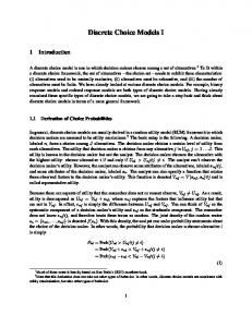
As a conclusion, if there are inertia and serial correlation effects, a mis-specified model (even if inertia dummies are included) might lead to bias in the coefficient estimates and produce significant response errors, especially in the case of strong policy changes. Thresholds in the Context of Minimum Perceptible Changes This context suggests that if a change in some attribute is small, the variation in the individual’s utility will be null. This is an important and contentious issue. We have been warned that it is possible to overestimate benefits of transport projects (e.g. time savings) because the impact of each unit saved below some critical threshold could amount to nothing for the individual (Welch and Williams, 1997). As an illustration, Figure 1 shows the variation in utility when the attribute Xk (with negative marginal utility) changes all things being equal. The threshold is equal to 5 in this case, so values of ∆Xk between −5 and 5 do not produce changes in utility; in contrast, utility is affected outside this interval. Note that here a symmetric threshold was assumed, but there is evidence that these effects may be asymmetric. An early model for these effects was proposed by Krishnan (1977), who used the concept of minimum perceivable difference within a conventional binary logit model, but assumed the individual was focused on total utility rather than on attribute partworths. Researchers in marketing have examined consumer price sensitivity using models that incorporate probabilistic thresholds for price gains and losses with respect to the reference price. Han et al. (2001) proposed the incorporation of a reference price RPjqt, and expressed the utility function as: Figure 1. Presence of thresholds as minimum perceptible change
U jqt = θX jqt + β loss ( Pjt − RPjqt )I jqt , loss + β gain ( RPjqt − Pjt )I jqt , gain + ε jqt
(12)
∆V j
0.08 0.06 0.04 0.02
∆X k
0 15
10
5
0.02
0
5
10
0.04 0.06 0.08 Figure 1.
Presence of thresholds as minimum perceptible change
15
Implications of Thresholds in Discrete Choice Modelling 677 where Pjt is the shelf price, Ijqt,loss = 1 if Pjt – RPjqt > τjqt,loss and 0 otherwise; similarly, Ijqt,gain = 1 if RPjqt – Pjt > τjqt,gain and 0 otherwise; τjqt,loss and τjqt,gain are thresholds for loss and gain respectively, and βgain and βloss are parameters to be estimated. For example, given a threshold, the change in the utility function may be as in Figure 2 where all things being equal τjqt,loss = 5, θshellprice = −0.03, βloss = −0.02 and the reference price was the shell price before the change, so ∆Pj = (Pj – RPj). On the other hand, Han et al. recognize that as thresholds9 have a deterministic and random component, they may be expressed as: Figure 2. Price threshold in the utility function according to Han et al. (2001)
τ jqt = αZ jqt + ζ jqt
(13)
where Zjqt is factors that may affect the threshold, α is a vector of parameters and ζjqt are random components. Then, the utility function (12) is modified as follows: U jqt = θX jqt + β loss ( Pjt − RPjqt ) Prob ( I jqt , loss = 1) +
β gain ( RPjqt − Pjt ) Prob ( I jqt , gain = 1) + ε jqt
(14)
where Prob(Ijqt,loss = 1) is the probability that (Pjt – RPjqt) > τjqt,loss and Prob(Ijqt,gain = 1) the probability that (RPjqt – Pjt) > τjqt,gain. Although the model considers that the marginal change in utility depends on the magnitude of change in attributes with stochastic thresholds, it does not correspond exactly to the concept defined in this section. Li and Hultkrantz (2000) proposed a bimodal model to estimate the value of time considering a stochastic perception threshold. In their approach, the utility difference function was written as: ∆U q = −α ( ∆tq − δ q ) − β∆ cq + ε q if δ q < ∆tq and ∆U q ≤ 0 otherwise
0.35
(15)
∆V j
0.30 0.25 0.20 0.15 ∆ Pj
0.10 0.05 0 –0.05 0
1
2
3
4
5
6
7
8
9
–0.10 –0.15
Figure 2.
Price threshold in the utility function according to Han et al. (2001)
10
678
V. Cantillo and J. de D. Ortu´zar
where ∆t and ∆c are the absolute time saving (delay) and that of the associate cost (compensation) for the willingness-to-pay (WTP)/to accept (WTA) model; α and β are parameters (α < 0 and β > 0 for the WTP model and the contrary for the WTA model), and δ is a non-negative stochastic threshold of travel time change. It is assumed that the individual will accept the proposed change if ∆Uq ≥ 0.10 This model was restricted to binary choice, assumed a uniformly distributed time threshold and no thresholds for the other attributes. Cantillo et al. (2005b) proposed a fairly general discrete choice model incorporating thresholds as minimum perceptible changes in attributes, considering multiple alternatives and allowing for changes in several attributes. They also postulated that if thresholds exist they could be random, differ among individuals, and even be a function of socio-economic characteristics and choice conditions. Their formulation allows estimating the parameters of the threshold probability distribution starting from information about choices. As a hypothesis, they suggest that if the change is small the variation in the individual’s systematic utility will be null. Therefore, the individual will only perceive an alteration in his/her utility if ∆Xˆ t + 1 ≥ δ , where δ is a non-negative random perception kjq
kq
kq
threshold that distributes with density function φ(δk) in the population. The indit +1 bigger than δ , so that response is to a vidual only perceives that part of ∆Xˆ kjq kq
(
)
stimulus of size Max ∆Xˆ t + 1 − δ , 0 . kjq kq To examine the effect of thresholds on a mispecified MNL model, Cantillo et al. (2005b) built a simulated database with three alternatives, and attributes as before. The data were generated considering that, initially, individuals chose according to a compensatory utility maximizing process (i.e. a MNL model with scale parameter equal to 1). Then, attributes changed and individuals compared these changes with their thresholds in turn; if the threshold was not exceeded the utility function did not change. They assumed a symmetric triangular threshold distribution starting at zero, so only one parameter defines it (i.e. mean or mode). Finally, individuals chose again among alternatives according to a compensatory utility maximizing process. The true parameters of the utility function used are presented in Table 5, together with the number of individuals for whom the change in either alternative surpassed the respective threshold for each simulated case. As can be seen, the threshold effect is strongest for the attribute Access Time and weakest for Cost. Similarly, Cost has the smallest marginal utility, and Access Time the largest. Table 5. Parameters used for threshold generation
Parameter
Cost Travel Time Access Time
Mean of threshold
0.08 0.12 0.16
Parameters in utility function
−0.070 −0.150 −0.200
Individuals whose threshold was surpassed by an attribute change (total sample = 10 000)
Alternative 1
Alternative 2
9680 6852 3166
5391 8124 3467
Implications of Thresholds in Discrete Choice Modelling 679 Eight scenarios were analysed in each case combining the presence or absence of thresholds (Table 6). For instance, the first scenario consisted of a population without thresholds in any attribute and the last scenario considered a population with thresholds for all attributes. In each case, a classical non-thresholds MNL model and the proposed model were estimated. Simulations showed that when the attribute changes increased the bias in the MNL parameters increased too. On the other hand, as the incidence of the Access Time threshold was stronger than the others, its estimation tended to be more successful. In general, the LR tests showed that the restricted MNL models were not equivalent to the threshold models. The response performance of both models for scenario 8 was also tested by Cantillo et al. (2005b). Again, in addition to the status quo, two ‘policy changes’ are shown here, a light one (Travel Time for Bus was decreased 20%), and a strong one (all the attributes for Metro increased 50%, and all the attributes for Bus decreased 50%). In this case, 10% was a reasonable tolerance error. Table 7 shows that in the status quo case response errors were not significant in either model. However, for both policies the MNL model gave rise to significant response errors while those of the proposed models were well within the tolerance level. Finally, in terms of response changes, we show that the MNL model significantly over predicts in the case of the strong policy, while the proposed model is accurate even in that case. Finally, the threshold model was applied to real data coming from a route choice SP survey for car trips (Caussade et al., 2005). The present paper selected a part of the survey with choices based on three attributes: Travel time (min), Trip time variability (min) and Total cost (US$). In the implementation of the experiment, respondents were first asked to consider a trip they had taken recently and to report its attributes (this was called Current Route). Then a computer program automatically generated the hypothetical choice scenarios according to a fractional factorial design. Each specific design pivoted on the attribute levels associated with the Current Route. As a generic design, the added options (two in the case of this data) were of exactly the same nature. Model TM in Table 8 includes a threshold for Travel Time assuming a uniform distribution (there was no evidence of thresholds for the other attributes). Clearly, model TM is significantly better than the reference MNL model (LR = 51.2 is substantially higher than 3.84, the critical value at the 5% level); consequently, it could be concluded that a threshold for Travel Time exists with a mean close to 11% of its initial value. Thus, it is possible to conclude again that if there is evidence about the existence of perception thresholds in the population, the use of models without them may lead to errors in estimation and in prediction. However, this occurs with more emphases when the incidence of a given attribute in the utility function is strong. On the other hand, threshold effects for several attributes can be confounded or even compensated. Thresholds in the Context of a Mechanism for the Acceptance or Rejection of an Alternative Although most discrete choice models have been based on the assumption that individuals choose following compensatory behaviour, people may actually behave non compensatory as in the elimination-by-aspects (EBA) process
−0.070
Cost
MNL
Proposed
142
√
2
MNL
Time
316
√
4
–
–
–
–
–
–
0.071 (4.4) [−0.5] 0.094 (6.6) [−1.8]
−0.196 −0.197 (−38.4) (−38.4) [0.8] [0.6]
−0.181 −0.196 (−35.5) (−35.4) [3.8] [0.7]
Proposed
−0.071 −0.070 (−47.7) (−46.3) [−0.6] [−0.1] −0.150 −0.149 (−53.1) (−52.0) [−0.1] [0.3]
MNL
179
√ √
5
−0.073 −0.071 (−47.1) (−46.8) [−1.6] [−0.6] −0.149 −0.146 (−52.5) (−52.1) [0.3] [1.4]
Proposed MNL Proposed
251
√
3
−0.071 −0.071 −0.069 −0.071 −0.072 −0.070 (−48.8) (−44.3) (−48.0) (−48.0) (−47.8) (−46.5) [−0.6] [−0.8] [0.6] [−0.3] [−1.4] [−0.3] Travel −0.150 −0.147 −0.147 −0.145 −0.147 −0.151 −0.148 Time (−53.0) (−51.2) (−53.1) (−53.6) (−53.1) (−51.2) [1.3] [1.1] [2.0] [1.2] [−0.4] [0.8] Access −0.201 −0.198 −0.199 −0.197 −0.200 −0.198 −0.197 Time (−39.1) (−39.0) (−39.5) (−39.7) (−38.3) (−38.1) [0.4] [−0.2] [0.5] [0.1] [0.6] [0.7] Mean 0.080 – 0.002 – 0.084 – – threshold (0.2) (9.0) Cost [0.2] [0.5] 0.120 – 0.000 – – – Mean 0.105 (0.0) threshold (7.0) [0.0] Travel [−1.0]
Proposed
Target
Model
MNL
0
1
Individuals changing their choice when threshold present
Cost Travel Time Access Time
Threshold
Scenario
Proposed
–
–
0.052 (4.5) [−2.4] –
−0.179 −0.193 (−35.4) (−30.3) [4.2] [1.1]
−0.072 −0.071 (−47.1) (−46.5) [−1.1] [−0.5] −0.147 −0.145 (−52.4) (−52.2) [1.1] [1.7]
MNL
247
√
√
6
Proposed
–
–
0.101 (9.8) [−1.9]
–
−0.177 −0.193 (−34.4) (−34.2) [4.6] [1.3]
−0.074 −0.071 (−46.8) (−45.2) [−2.3] [−0.3] −0.152 −0.147 (−53.3) (−51.2) [−0.6] [1.2]
MNL
544
√ √
7
Table 6. Effect of the presence of threshold for change perceptible in attributes on model estimation
Proposed
–
–
0.059 (4.1) [−1.4] 0.090 (4.1) [−1.4]
−0.178 −0.193 (−34.7) (−34.0) [4.4] [1.2]
−0.073 −0.071 (−46.9) (−44.9) [−2.2] [−0.6] −0.150 −0.147 (−52.3) (−49.1) [−0.1] [1.1]
MNL
427
√ √ √
8
680 V. Cantillo and J. de D. Ortu´zar
MNL, Multinomial logit model.
0.2 7.81
−5751.8 −5751.7
Loglikelihood
LR test Critical χ2 at the 5% level
–
0.160 Mean threshold Access Time
0.008 (1.2) [1.2]
Proposed
MNL
Model
Target
0
Individuals changing their choice when threshold present
−5859.5
–
MNL
15.3 3.84
−5851.8
–
Proposed
142
316
–
34.9 3.84
0.149 (13.7) [−1.0]
45.8 3.84
−5512.8 −5489.9
–
Proposed MNL Proposed
−5595.3 −5577.9
–
MNL
251
−5654.4
–
MNL
Table 6. Continued
15.5 5.99
−5646.7
–
Proposed
179
−5581.4
–
MNL
21.3 5.99
−5570.8
0.128 (3.0) [−0.8]
Proposed
247
0.162 (10.6) [0.1]
Proposed
133.6 5.99
−5380.9 −5314.1
–
MNL
544
0.150 (10.6) [−0.7]
Proposed
71.7 7.81
−5427.2 −5391.3
–
MNL
427
Implications of Thresholds in Discrete Choice Modelling 681
682
V. Cantillo and J. de D. Ortu´zar Table 7. Simulated and modelled forecasts for thresholds as minimum perceptible change Multinomial logit (MNL) model
Targets Policy
Taxi
Status quo Error (%) Light Error (%) Change (%) Strong Error (%) Change (%)
110
110
779
108
147
745
Bus
Metro
−1.8 3.1 −4.4 63 832 105 −42.7 656.4 −86.5
Taxi
Bus
94 −14.5 87 −19.4 −7.5 52 −17.5 −73.4
103 −6.4 164 11.6 5.9 874 5.0 748.5
Metro
χ2
803 3.5 3.1 749 6.1 0.5 −6.7 74 13.2 −29.5 −90.8
Proposed model Taxi
Bus
Metro
χ2
106 −3.6 100 −7.4 −5.7 60 −4.8 −43.4
110 0.0 155 5.4 4.1 839 0.8 619.0
785 0.8 745 0.0 −5.1 101 −3.8 −87.1
0.2 1.0
0.4
(Tversky, 1972; Young et al., 1982) or the satisficing heuristic (Simon, 1955). More than 20 years ago, Williams and Ortúzar (1982) verified the inconsistency of parameters estimated using standard models when people behaved in noncompensatory fashion or if individual choice sets were incorrectly specified. In typical discrete choice model applications, the modeller assumes that choice sets can be established deterministically. The availability of an alternative is treated as an observable binary variable defined based on often arbitrary criteria (i.e. a mode is available if its access time is less than certain duration). Thus, even though the modeller accepts that a threshold may exist, he does not consider individual differences that could imply that for some people an alternative might still be available (i.e. people may be prepared to walk more than a predefined duration criteria to board a vehicle). In this case, the utility function may be as shown in Figure 3, where utility falls to minus infinite when a threshold is surpassed. Some analysts have centred their attention on the choice set formation process based on the two-stage choice paradigm and probabilistic choice set model presented by Manski (1977), who suggested that: Figure 3. Thresholds in attributes
Ptq =
∑ Pq (i / C)Pq (C / G)
(16)
C ∈G
where Piq is the probability that individual q chooses option Ai (Ai ∈ M); M is the master set of alternatives; Pq(i/C) is the probability that individual q chooses Ai given choice set C; and Pq(C/G) is the probability that the choice set of individual q is C. In this case G is the set of all non-empty subsets of M or, what is the same, all Table 8. Models for the stated preference (SP) survey Parameters (t-ratios)
Multinomial logit (MNL) model
Model TM
Travel Time Variability Cost Mean threshold Travel Time Sample size Log-likelihood
−0.0353 (−14.8) −0.0146 (−3.4) −0.2100 (−8.7) – 782 −623.2
−0.1221 (−8.3) −0.0169 (−3.1) −0.420 (−8.9) 0.1106 (17.8) 782 −597.6
Implications of Thresholds in Discrete Choice Modelling 683
U
threshold
Xk
Ð∞ Figure 3.
Thresholds in attributes
the potential choice subsets. In general, if M has nq options, G has a maximum of elements. Swait and Ben Akiva (1987) incorporated random constraints in discrete models of choice set generation. If the value of an attribute, Xjqk, is larger that a certain threshold Txkq, the individual will reject alternative Aj. Thus, in this behavioural model an individual will consider that an alternative is part of her choice set if and only if all its attributes are within their respective thresholds. Thresholds are considered independent here, so the probability that Aj is included in the choice set of individual q is given by: Kj
(
)
Pq , j ∈C = ∏ Prob X jqk ≤ TX kq , k =1
(17 )
Obviously, the probability that alternative Aj does not belong to choice set C is given by Pq , j ∉C = 1 − Pq , j ∈C , and the probability that the choice set is empty is equal to the probability that no alternative belongs to it. The choice set formation is modelled as: n
{
}
q 1 (1 − d ) d Pq (C / G) = ∏ Pq , jCj ∈C ⋅ Pq , j ∉CjC , 1 − Pq , C = φ j = 1
(18)
where djC is one if Aj is an element of choice set C, and zero otherwise. The conditional choice Pq(i/C) is modelled according to RUT. The main problem of the approach is the high degree of computational complexity associated to a large number of alternatives (more than six). Morikawa (1995) suggests an appropriate method when M consists of too many alternatives, whereby the set formation process is modelled by pair-wise comparisons of alternatives, reducing the computational effort. Following a similar approach, Ben Akiva and Boccara (1995) discussed models with latent choice sets, by adding an explicit probabilistic representation of the various alternatives considered by the individual. They incorporated the effects of stochastic constraints or elimination criteria, and the influence of attitudes and perception on the choice set generation process. Their idea was to estimate a choice set generation model using information contained in the response to questions about the availability of each alternative. Therefore, the use of this approach
684
V. Cantillo and J. de D. Ortu´zar
demands additional information related to responses to alternative availability questions. Other approaches have considered the extent to which choice set formation and choice (given the choice set) can be identified separately (Smith et al., 1991; Scrogin et al., 2004), defining an efficient frontier function. In these models, individual choice sets may be defined in terms of the efficiency of alternatives in the universal choice relative to the frontier function. Cascetta and Papola (2001) proposed a random utility model based on the concept of intermediate degrees of availability/perception of alternatives, simulated through an ‘inclusion function’ introduced in the systematic utility. They proposed a modification in (1) by including a term ln(µjqC), where µjqC is a continuous variable defined over the interval (0,1) representing the degree of membership of alternative Aj to choice set C. A good approach to µjqC considering thresholds for attributes is given by (17). With this approach, the utility function would be: U jq = Vjq + ln( Pq , j ∈C ) + ε jq
(19)
which is estimated using maximum likelihood methods, and does not need the two-stage process. In fact, the latter is the main advantage of this approach but the microeconomic support to include the new term in the utility function is not clear. A model that suggests an extension of the traditional compensatory utility maximization framework was proposed by Swait (2001), who incorporated limits in the value of the attributes in the formulation of the decision problem. Reference is made to an individual having marginal utilities that can change according to the value that a specific attribute takes according to pre-established thresholds (Figure 4). According to this approach, each attribute k has a lower cut-off or threshold τLkq, and an upper threshold τUkq, and the utility function is expressed as: U jq = θX jq + θ L δ Ljq (τ Lq − X jq ) + θ U δ Ujq (X jq − τ Uq ) + ε jq
(20)
where δLjq is a diagonal matrix with the element kk = 1 if Xjqk < τLkq and zero otherwise; similarly, the kk element in δUjq = 1 if Xjqk > τUkq and zero otherwise. Figure 4. Utility variation incorporating limits in attribute values
U
thresholds
Xjkq Figure 4.
Utility variation incorporating limits in attribute values
Implications of Thresholds in Discrete Choice Modelling 685 The cut-offs are obtained from a survey (individuals are asked directly about them), and the parameters θU and θL are estimated. The EBA model is a limiting case where for an attribute k (with negative marginal utility) the lower threshold does not exist and θU is minus infinity. In its simplest form, this model can be estimated using standard software; in fact, in the SP experiment analysed by Swait (2001) individuals identified the attribute thresholds that were treated as exogenous variables. However, the estimation of the model based only on choices with thresholds treated as endogenous variables, cannot be done using standard software. Gilbride and Allemby (2004) proposed a model that allows considering conjunctive, disjunctive and compensatory screening rules. In this approach, if Tq is a vector of random thresholds,11 the alternatives included in the choice set are identified with an indicator function, I(Xjq,Tq) that is equal to 1 if the decision rule is satisfied and zero otherwise, then the choice model can be written in general form as: Piq = P(Viq + ε iq ≥ Vjq + ε jq for all j such that I (X jq , Tq ) = 1)
( 21)
In the case of a conjunctive rule an alternative is acceptable if all its relevant attributes are acceptable; then, the indicator function12 is ΠkI(Xjkq ≤ Tkq) = 1; meanwhile, in a disjunctive decision rule if at least one of the attribute levels is acceptable, then ΣkI(Xjkq ≤ Tkq) = 1. The model can be estimated using the Bayesian technique of data augmentation and Markov-Chain Monte Carlo methods to integrate over the parameter space. Although complex to estimate, the model reflexes resurgence in these topics. Cantillo and Ortúzar (2005) proposed a model inspired in the two-stage paradigm considering correlation among thresholds. Also, if thresholds exist they can be random, differ among individuals and also be a function of socio-economic features and choice conditions. Their formulation allows estimating both the model taste parameters and those of the threshold probability distribution. Here thresholds distribute according to a join density function Ω(δ) with mean E[Tq]=T¯ and covariance matrix Var[Tq]=Σ, then the probability Pq,j∈C = P{Xqj ≤ Tq}, and this can be written as:
{
∞
∞
∞
} ∫ ⋅⋅ ∫ ∫
Pq , j∈C = P X qj ≤ Tq =
Ω(δ ) dδ 1dδ 2 L dδ k
(22)
X kjq X 2 jq X 1 jq
This approach is more general allowing for correlation among thresholds and an explicit estimation of the threshold distribution parameters. They also proposed expressing the thresholds’ means as a linear function of the individual’s socioeconomic characteristics. To examine the effect of thresholds in this sense, a simulated databank with the same three hypothetical alternatives and attributes than in the two examples discussed previously was generated. The simulated population choice process proceeded comparing each attribute with its threshold in turn; if the threshold was exceeded the alternative under consideration was rejected. Then, if two or more alternatives were accepted after the first stage, the individual had to choose among them according to a compensatory utility maximizing process. The ‘true’ (target) parameters of the utility function are presented in Table 913 together with the results of estimating three types of models. The first is a
686
V. Cantillo and J. de D. Ortu´zar Table 9. Effect of attribute threshold on model estimation
Parameters (t-ratios)
Parameter target
Multinomial logit (MNL) model
Mixed logit (ML)
Proposed model
−0.005 −0.08 −0.16 40 5
−0.0808 (−53.1; 49.8) −0.0714 (−45.1; 5.4) −0.1618 (−44.7; 0.5) – –
−0.0808 (−53.1: 49.8) −0.0714 (−45.1: 5.4) −0.1619 (−44.7; 0.5) – –
−0.0074 (−1.81; 0.6) −0.0805 (−22.8; 0.1) −0.1647 (−31.4; 0.9) 40.2 (118.4; 0.6) 5.3 (24.1; 1.4)
45
–
–
45.8 (26.7; 0.5)
8
–
–
10.5 (6.2; 1.5)
28
–
–
27.9 (32.2; 0.1)
4
–
–
3.0 (4.2; 1.4)
–
0.00 (0.01)
–
–
0.0003 (0.07)
–
–
0.0002 (0.03)
–
10 000 −7523.0
10 000 −7523.0
10 000 −6944.9
Cost Travel Time Access Time Mean threshold Cost Standard deviation threshold Cost Mean threshold Travel Time Standard deviation threshold Travel Time Mean threshold Access Time Standard deviation threshold Access Time Standard deviation Cost (σC) Standard deviation Travel Time (σTT) Standard deviation Access Time (σAT) Sample size Log likelihood
10 000
classical MNL model fully consistent with compensatory behaviour; the second is a mixed logit (ML) model allowing for a Normally distributed random taste parameters and the last is the proposed model. First, it is important to note that even the flexible specification of random parameters in the ML model does not allow compensating for the existence of thresholds, as the ML is clearly indistinguishable from the MNL. Second, the t-tests show that their parameters for Cost and Travel Time are significantly different from the targets at the 95% level. On the other hand, although the estimation of subjective values of time (SVT) from the compensatory models is biased as can be seen in Table 10, the proposed model recovers parameters well and of the SVT estimates are well within their confidence intervals. Table 10. Effect of attribute threshold on subjective values of time (SVT) Multinomial logit (MNL) model
SVT Travel Time Access Time
Proposed model
Target
Point estimate
Confidence interval
Point estimate
Confidence interval
16.0 32.0
0.88 2.00
0.84–0.92 1.94–2.06
10.9 22.3
5.48–120.0 11.7–234.9
Implications of Thresholds in Discrete Choice Modelling 687 Finally, Cantillo and Ortúzar (2005) also tested the performance of the MNL and the proposed model in terms of their predictive capabilities through scenarios representing various ‘policy changes’. For the light policy, Travel Time for Bus was decreased 20%; meanwhile, in the strong policy Cost for Metro was increased 100%. In this case, 3% was found to be a reasonable error tolerance. Table 11 shows that the MNL gave response errors larger than the tolerance, even in the status quo scenario. A similar analysis using the χ2 index showed that the MNL errors were significant in all cases. In contrast, predictions using the proposed model were well within their tolerances. These findings are complemented by the response change forecasts; as can be seen, the MNL model significantly over predicts in the case of the strong policy whilst the proposed model performs accurately. The MNL problems in this case are well-known and had been documented a long time ago (Williams and Ortúzar, 1982). Finally, the effect of having correlated thresholds was also tested and evidence suggested that in the estimation of a choice model incorporating thresholds, the effect of threshold correlation may only be marginal. The threshold model was also applied to real data coming from a route choice SP survey for car-trips between the cities of Santiago and Valparaiso, Chile (Rizzi and Ortúzar, 2003). Three variables were used in the experiment: travel time (min), toll charge (US$) and number of fatal accidents per year. Each individual had to choose between the two routes according to a fractional factorial design. Several models were analysed assuming that the thresholds were independent and followed a left truncated Normal distribution; however, there was only evidence of threshold effects for the attribute Accidents. In the threshold model T (Table 12) the mean of the threshold for Accidents is expressed as τ + ρY; the latter is a dummy variable that takes the value one for men of 30 years old or less, and zero otherwise. This function was based on evidence that males under this age were less likely to be willing to pay for safety (Rizzi and Ortúzar, 2003). The results indicate that all the effect of the Accidents variable appears at the non-compensatory stage, acting as a discriminating element. Contrariwise, both Toll and Travel time are clearly more relevant at the compensatory stage. On the other hand, the LR test (43.3) implies a definitive threshold effect for Accidents. Note that the parameter of this attribute in the utilities of model T has a positive sign but low t-ratio, suggesting it could be Table 11. Simulated and modelled forecasts in the presence of attribute thresholds Multinomial logit (MNL) model
Targets
χ2
Policy
Taxi
Bus
Metro
Taxi
Status quo Error (%) Light Error (%) Change (%) Strong Error (%) Change (%)
1590
2733
5677
1451
3602
4947
−8.7 1658
31.8 2973
−12.9 5369
4.3
8.8
−5.4
1380 2686 5934 40.3 −13.2 −1.7 4.5 1241 3359 5399 88.0 −14.5 −6.7 9.1 −10.1 25.1 −9.0 2226 4173 3601 1260.7 34.3 40.3 −32.9 61.3 55.4 −39.3
Bus
Metro
Proposed model Taxi
Bus
Metro
χ2
1583 −0.4 1455 0.3 −8.1 1665 0.4 5.2
2738 0.2 3610 0.2 31.8 3001 0.9 9.6
5678 0.0 4935 −0.2 −13.1 5334 −0.6 −6.1
0.0 0.1
0.5
688
V. Cantillo and J. de D. Ortu´zar
Table 12. Models for the stated preference (SP) survey including all individuals Parameters (t-ratios)
Range
Accidents Toll charge Travel time Mean threshold Accidents Standard deviation threshold Accidents Young men (ρ) Sample size Log-likelihood
16–28 2.4–7.0 90–135
Multinomial logit (MNL) model
Model T
−0.1028 (−14.7) −0.35 (−7.9) −0.0391 (−14.4) – –
0.0262 (0.7) −0.50 (−5.3) −0.0673 (−7.1) 28.14 (41.9) 5.85 (6.9)
– 3071 −1795.5
6.30 (2.8) 3071 −1773.3
dropped from the specification. Finally, the positive sign and magnitude of the extra parameter ρ allowed concluding that the accident threshold for young men was larger than for the rest of the population. So, as in the previous cases, we are able to conclude that if there is evidence about the existence of thresholds in the population the use of a mis-specified compensatory model, such as MNL or even ML, can lead to significant errors in predictions and in estimation even in the case of relatively mild policy changes. Moreover, results seem to indicate that this type of thresholds appear to be more important for model quality than the previous two. Conclusions The paper reviewed the consideration of thresholds in discrete choice models in three contexts: inertia, minimum perceptible change and as a mechanism of acceptance or rejection of alternatives. As there are solid psychological foundations supporting the presence of thresholds, there is a challenge for the modeller to understand and formulate models with greater realism in the representation of how individuals actually process the choice tasks. Although each kind of threshold was discussed independently, they might occur simultaneously and their effects overlap. This is a very interesting topic to be researched. Some of the findings of the analysis are consistent with those of previous research. For example, if there is evidence about the existence of thresholds in the population, a mispecified model without thresholds will have a biased parameter and produce significant response errors in forecast, especially in the case of strong policy changes. Preliminary applications show that thresholds in the context of a mechanism for the acceptance or rejection of an alternative appear more important for model quality than the other two thresholds, but additional evidence is required to support this conclusion. Although the inclusion of thresholds increases the complexity of the modelling task, the additional effort improves model accuracy, enhancing the representation of individual choice-making behaviour. On the other hand, recent developments in numerical techniques and computer power allow for a relatively easy estimation of these models. An interesting topic for further research is the consideration of models including several types of thresholds (e.g. thresholds for inertia and minimum perceptible changes). Of course, this adds complexity to the model and implies the
Implications of Thresholds in Discrete Choice Modelling 689 necessity of considering two main problems. The first is related to the important theme of parameter identification; the second is related to the sample size requirements to estimate the parameters correctly. Acknowledgements The authors are grateful to Elisabetta Cherchi, Ben Heydecker, Luis Ignacio Rizzi and Huw Williams for help in developing these ideas. The useful comments of two anonymous referees are also appreciated. Notwithstanding, and as usual, all errors are the sole responsibility of the authors. Thanks are also due to the Chilean Fund for the Development of Scientific and Technological Research (FONDECYT) for having supported this research through several projects (1970117, 1000616 and 1020981). Notes 1. Decision strategies that use trade-offs among attributes are called compensatory strategies (Payne et al., 1993). 2. A similar approach to consider an agent effect includes capturing correlation among responses for a given individual, as proposed by Morikawa et al. (1995). 3. An interesting topic is the identification problem. If one has a panel (at least two responses per person), for J = 2, only one parameter in ν can be identified, but if J ≥ 3, one can estimate all the parameters. 4. The LR statistic −2{l*(θr) – l*(θ)},where l*(θ) and l*(θr) are the log-likelihood at convergence for the non-restricted and the restricted model, respectively, is asymptotically distributed χ2 with r degrees of freedom, where r is the number of linear restrictions (Ortúzar and Willumsen, 2001). 5. Very large sample sizes are necessary to recover the parameters of even much simpler models with simulated data (Williams and Ortúzar, 1982; Munizaga et al., 2000) 6. The authors are grateful to a referee for pointing this out; for a detailed explanation of this effect, see Sillano and Ortúzar (2005). 7. The user was asked to provide a simple judgement of the comfort experienced during the journey described. The variable was pre-coded into three levels: poor, sufficient and good; and two dummy variables were used: Comf1 = 1 if the level of comfort was poor, and Comf2 = 1 if comfort was sufficient. As the ‘good’ level was left as a reference, it was implicit that car had high comfort. 8. Cherchi and Ortúzar (2002) also tried an inertia variable following the approach of Bradley and Daly (1997), but it was clearly not significantly different from zero. 9. This is not exactly a threshold approach as defined in this section, but a representation of framing using a reference price that introduces asymmetry. The authors are grateful to a referee for pointing this out. 10. The model assumes that the error term is invariant in time. 11. As rightly pointed out by a referee, according to this notation, the vector of thresholds for individual q does not vary across alternatives. However, it is possible to define alternative specific thresholds (e.g. the thresholds on access or travel time for public transport and car might be different). 12. Assuming independence among thresholds. 13. To generate the synthetic data, no alternative specific constants were included, but there is no identification problem for the alternative specific constants due to the presence of thresholds.
References Armstrong, P. M., Garrido, R. A. and Ortúzar, J. de D. (2001) Confidence intervals to bound the value of time, Transportation Research, 37E, pp. 143–161. Ben Akiva, M. and Morikawa, T. (1990) Estimation of switching models from revealed preferences and stated intentions, Transportation Research, 24A, pp. 485–495. Ben Akiva, M. E. and Boccara, B. (1995) Discrete choice models with latent choice sets, International Journal of Research in Marketing, 12, pp. 9–24.
690
V. Cantillo and J. de D. Ortu´zar
Bradley, M. A. and Daly, A. J. (1997) Estimation of logit models using mixed stated preference and revealed preference information, in: P. R. Stopher and M. Lee-Gosselin (Eds), Understanding Travel Behaviour in an Era of Change, pp. 209–232 (Oxford: Pergamon). Cantillo, V., Heydecker, B. and Ortúzar, J. de D. (2005b) A discrete choice model incorporating thresholds for perception in attribute values, Transportation Research, B (in press). Cantillo, V. and Ortúzar, J. de D. (2005) A semi-compensatory discrete choice model with explicit attribute thresholds of perception, Transportation Research, 39B, pp. 641–657. Cantillo, V., Ortúzar, J. de D. and Williams, H. C. W. L. (2005a) Modelling discrete choices in the presence of inertia and serial correlation, Transportation Science (submitted). Cascetta, E. and Papola, A. (2001) Random utility models with implicit availability/perception of choice alternatives for the simulation of travel demand, Transportation Research, 9C, pp. 249–263. Caussade, S., Ortúzar, J. de D., Rizzi, L. I. and Hensher, D. A. (2005) Assessing the influence of design dimensions on stated choice experiment estimates, Transportation Research, 39B, pp. 621–640. Cherchi, E. and Ortúzar, J. de D. (2002) Mixed RP/SP models incorporating interaction effects: modelling new suburban train services in Cagliari, Transportation, 29, pp. 371–395. Daganzo, C. F. and Sheffi, Y. (1979) Estimation of choice models from panel data, paper presented at the 26th Annual Meeting of the Regional Science Association, Los Angeles, CA, USA, November 1979. Daganzo, C. F. and Sheffi, Y. (1982) Multinomial probit with time-series data: unifying state dependence and serial correlation models, Environment and Planning, 17A, pp. 1377–1388. Gilbride, T. and Allemby, G. (2004) A choice model with conjunctive, disjunctive and compensatory screening rules, Marketing Science, 23, pp. 391–406. Goodwin, P. W. (1977) Habit and hysteresis in mode choice, Urban Studies, 14, pp. 95–98. Greene, W. and Hensher, D. (2003) A latent class model for discrete choice analysis: contrast with mixed logit, Transportation Research, 37B, pp. 681–698. Guadagni, P. and Little, J. (1983) A logit model of brand choice calibrated on scanner data, Marketing Science, 2, pp. 203–238. Han, S., Gupta, S. and Lehmann, D. (2001) Consumer price sensitivity and price thresholds, Journal of Retailing, 77, pp. 435–456. Heckman, J. (1981) Statistical models for discrete panel data, in: C. F. Manski and D. McFadden (Eds), Structural Analysis of Discrete Data: With Econometric Applications, pp. 114–178 (Cambridge, MA: MIT Press). Hirobata, Y. and Kawakami, S. (1990) Modelling disaggregate behavioural modal switching based on intention data, Transportation Research, 24B, pp. 15–25. Johnson, L. and Hensher, D. (1982) Application of multinomial probit to a two-period panel data set, Transportation Research, 16A, pp. 457–464. Kitamura, R. (1990) Panel analysis in transportation planning: an overview, Transportation Research, 24A, pp. 401–415. Krishnan, K. S. (1977) Incorporating thresholds of indifference in probabilistic choice models, Management Science, 23, pp. 1224–1233. Li, C.-Z. and Hultkrantz, L. A. (2000) Stochastic threshold model for estimating the value of travel time, paper presented at the Annual Conference, Rethymnon, Greece. Manski, C. F. (1977) The structure of random utility models, Theory and Decisions, 8, pp. 229–254. McFadden, D. (2001) Disaggregate behavioural travel demand’s RUM side: a 30-year retrospective, in: D. Hensher (Ed.), Travel Behaviour Research: The Leading Edge, pp. 17–63 (London: Pergamon). McFadden, D. and Train, K. (2000) Mixed MNL models for discrete response, Journal of Applied Econometrics, 15, pp. 447–470. Morikawa, T. (1994) Correcting state dependence and serial correlation in the RP/SP combined estimation method, Transportation, 21, pp. 153–165. Morikawa, T. (1995) A hybrid probabilistic choice set model with compensatory and non-compensatory choice rules, in Proceedings of the 7th World Conference on Transport Research, Vol. 1: Travel Behaviour (Oxford: Pergamon). Morikawa, T., Ben-Akiva, M. and McFadden, D. (1995) Discrete choice models incorporating revealed preferences and psychometric data, Econometric Models in Marketing: A Research Annual, 12, pp. 29–55. Munizaga, M. A., Heydecker, B. G. and Ortúzar, J. de D. (2000) Representation of heteroscedasticity in discrete choice models, Transportation Research, 34B, pp. 219–240. Ortúzar, J. de D. and Willumsen, L. G. (2001) Modelling Transport, 3rd Edn (Chichester: Wiley). Payne, J., Bettman, J. and Johnson, E. (1993) The Adaptive Decision Maker (New York, NY: Cambridge University Press).
Implications of Thresholds in Discrete Choice Modelling 691 Pendyala, R. M, Parashat, A. and Muthyalagari, G. R. (2000) Measuring day-to-day variability in travel characteristics using GPS data, paper presented at the 79th Annual Meeting of the Transportation Research, Board, Washington, DC, USA. Rizzi, L. I. and Ortúzar, J. de D. (2003) Stated preference in the valuation of interurban road safety, Accident Analysis and Prevention, 35, pp. 1–14. Scrogin, D., Hofler, R., Boyle, K. and Milon, J. W. (2004) An Efficiency Approach to Choice Set Generation. Working Paper, Department of Economics, University of Central Florida. Sillano, M. and Ortúzar, J. de D. (2005) Willingness-to-pay estimation with mixed logit models: some new evidence, Environment and Planning, 37A, pp. 525–550. Simon, H. A. (1955) A behavioural model of rational choice, Quarterly Journal of Economics, 69, pp. 99–118. Smith, V. K., Palmquist, R. B. and Jakus, P. (1991) Combining Farrell frontier and hedonic travel cost models for valuing estuarine quality, Review of Economics and Statistics, 73, pp. 694–699. Swait, J. D. (2001) A non-compensatory choice model incorporating attribute cut-offs, Transportation Research, 35B, pp. 903–928. Swait, J. D., Adamowicz, W. and Van Bueren, M. (2004) Choice and temporal welfare impacts: incorporating history into discrete choice models, Journal of Environmental Economics and Management, 47, pp. 94–116. Swait, J. D. and Ben Akiva, M. E. (1987) Incorporating random constraints in discrete models of choice set generation, Transportation Research, 21B, pp. 91–102. Train, K. (2003) Discrete Choice Methods with Simulation (Cambridge: Cambridge University Press). Tversky, A. (1972) Elimination by aspects: a theory of choice, Psychological Review, 79, pp. 281–299. Verplaken, B., Aarts H., Van Knippenberg, A. and Van Knippenberg, C. (1997) Habit, information acquisition and the process of making travel mode choices, European Journal of Social Psychology, 27, pp. 539–560. Welch, M. and Williams, H. C. W. L. (1997) The sensitivity of transport investment benefits to the evaluation of small time savings, Journal of Transport Economics and Policy, 31, pp. 231–254. Williams, H. C. W. L. and Ortúzar, J. de D. (1982) Behavioural theories of dispersion and the misspecification of travel demand models, Transportation Research, 16B, pp. 167–219. Young, W., Richardson, A. J., Ogden, K. W. and Rattray A. L. (1982) Road and rail freight mode choice: application of an elimination by aspects model, Transportation Research Record, 838, pp. 38–44.