Computer Vision and Image Understanding 80, 295–314 (2000) doi:10.1006/cviu.2000.0875, available online at http://www.idealibrary.com on
Implicit and Nonparametric Shape Reconstruction from Unorganized Data Using a Variational Level Set Method Hong-Kai Zhao1 Department of Mathematics, University of California, Irvine, California 92697-3875 E-mail:
[email protected]
and Stanley Osher,2 Barry Merriman,2 and Myungjoo Kang2 Department of Mathematics, University of California, Los Angeles, California 90095-1555 Received February 12, 1999; accepted August 3, 2000
In this paper we consider a fundamental visualization problem: shape reconstruction from an unorganized data set. A new minimal-surface-like model and its variational and partial differential equation (PDE) formulation are introduced. In our formulation only distance to the data set is used as our input. Moreover, the distance is computed with optimal speed using a new numerical PDE algorithm. The data set can include points, curves, and surface patches. Our model has a natural scaling in the nonlinear regularization that allows flexibility close to the data set while it also minimizes oscillations between data points. To find the final shape, we continuously deform an initial surface following the gradient flow of our energy functional. An offset (an exterior contour) of the distance function to the data set is used as our initial surface. We have developed a new and efficient algorithm to find this initial surface. We use the level set method in our numerical computation in order to capture the deformation of the initial surface and to find an implicit representation (using the signed distance function) of the final shape on a fixed rectangular grid. Our variational/PDE approach using the level set method allows us to handle complicated topologies and noisy or highly nonuniform data sets quite easily. The constructed shape is smoother than any piecewise linear reconstruction. Moreover, our approach is easily scalable for different resolutions and works in any number of space dimensions. °c 2000 Academic Press
1 2
Research supported by NSF DMS-9706566. Research supported by NSF and DARPA under Grants NSF DMS-9706827 and NSF DMS-9615854. 295 1077-3142/00 $35.00 c 2000 by Academic Press Copyright ° All rights of reproduction in any form reserved.
296
ZHAO ET AL.
1. INTRODUCTION The problem of shape reconstruction from an unorganized data set has many important applications in medical imaging, scientific computing, computer vision/graphics, and range images. The main challenge, especially in three and higher dimensions, is that neither the connections between the data points nor the topology of the final shape is known a priori. Most previous approaches can be classified as parametric or nonparametric (implicit surfaces). Parametric approaches in computational geometry usually use Voronoi diagrams and Delaunay triangulations to find connections between the data points and then construct a triangulated surface by connecting adjacent vertices. There has been much work in this area, for example [2–4, 7, 16, 17]. Finding the right connections among all the data points in three and higher dimensions is generally a challenging problem. Noise in the data and highly nonuniformly sampled data are also difficult to handle. There are also parametric approaches using variational or PDE methods [6, 12, 21] where a nice global parametrization is needed. Such a parametrization is almost impossible to obtain for complicated topologies. In general, the parametric form lacks depth information and requires a global parametrization which makes shape deformations and topological changes difficult to handle. In recent years the use of implicit surfaces and volumetric methods has attracted much attention [5, 8, 15, 18, 19]. In these approaches a scalar field function is constructed on a fixed grid and the final shape is a particular level set of the field function. Usually the scalar function is the signed distance to the final shape. Implicit representations usually have topological flexibility, a simple data structure, and depth/volumetric information. Such representations can also have memory space efficiency if properly managed [15]. Moreover, with the use of the signed distance representation, many surface tasks such as Boolean operations, ray tracing for illuminations, and computing offsets become quite simple. In this paper we introduce a nonparametric variational and PDE formulation. We use a continuous deformation to find the solution. In our numerical computations the level set method [23] is used to capture the deformation of implicit surfaces and to find the signed distance to the reconstructed shape. In Section 2 we first introduce the variational formulation which leads to a minimal-surface-like model. (We drop the suffix “like” in what follows, for simplicity of exposition.) The energy functional in our model involves a weighted surface area; i.e., it consists of a balance of elastic energy (surface area) and potential energy (distance to the data set). In Section 3 we calculate the gradient flow of our energy functional. We start with an initial surface that encloses the data set and uses a continuous deformation which follows the gradient flow to find the solution. In Section 4 we briefly review the level set method and derive its variational formulation for our problem. We show that the level set method provides a natural tool for capturing dynamic deformations of implicit surfaces. In Section 5 details of the numerical implementation are presented. A very efficient and robust PDE-based numerical algorithm is introduced to find the function which is the absolute distance to the data set on a rectangular grid. A good initial surface for our dynamic procedure is obtained using a level contour of this distance function. Numerical techniques for the level set method and for a multiresolution framework are also discussed. Finally, in Section 6, numerical examples are presented. In the Appendix we present a rigorous analysis of our model. Important features of our approach are as follows: 1. We use a variational and PDE-based formulation that only depends on the distance to a general data set that can include points, curves, and surface patches. Moreover, we have a very efficient PDE-based numerical algorithm to find this distance function.
SHAPE RECONSTRUCTION FROM DATA
297
2. The nonlinear regularization in our minimal surface model, which involves curvature, has an adaptive scaling property that allows varying flexibility. The constructed shape is smoother than any piecewise linear approximation in three and higher dimensions. 3. Numerically, we use the level set method on rectangular grids to find an implicit representation using the signed distance to the reconstructed shape. 4. Complicated topologies and noisy or nonuniform data sets can be handled easily. 5. Our method is easily scalable for multiple resolutions and works in any number of space dimensions. It can also be used as a smoothing procedure to postprocess other piecewise linear approaches. 2. THE MINIMAL SURFACE MODEL Let S denote the data set. In our formulation, S can include points, pieces of curves, and surfaces. The technique might also be generalized to reconstruct curves in R 3 using a new vector-valued level set method designed in [10]. Define d(x) = dist(x, S) to be the distance function to S. From now on we use boldface characters for vectors. We define the following surface energy for our variational formulation: ¸1/ p
·Z E(0) =
d p (x) ds 0
.
(1)
Here 0 is an arbitrary surface and ds is the surface area. The energy functional is independent of parametrization and invariant under rigid transformation. If we think of the distance function as a potential function for S, then our energy is the L p norm of the potential on 0. For a general data set the distance function is the only intrinsic information we have. When p = ∞, E(0) is the value of the distance of the most remote point on 0. We try to find a local minimizer of our energy functional that behaves like a minimal surface or an elastic membrane attached to the data set. We can easily calculate the first variation of the surface energy with respect to a small perturbation of 0, 1 δ E(0) = δ0 p
·Z
¸1/ p−1 d p (x) ds
0
[ pd p−1 ∇d · n + d p κ].
(2)
Here n is the unit normal and κ is the mean curvature of 0. The first term in the last square bracket above corresponds to a variation in the potential and the second term corresponds to a variation in the surface area. Hence the Euler–Lagrange equation is ·
d
p−1
¸ 1 (x) ∇d(x) · n + d(x)κ = 0. p
(3)
This PDE is well defined except at kinks of d(x) and the solution is interpreted as the viscosity solution [14] of the level set PDE defined in (9) below. We can see a balance between the potential force ∇d(x) · n (to minimize the potential energy) and the surface tension d(x)κ (to minimize the surface energy). Moreover, the nonlinear regularization due to surface tension has a desirable scaling d(x). Thus our membrane is more flexible close to the data and is more rigid away from the data. Equation (3) enforces a local condition for
298
ZHAO ET AL.
the sampling density; i.e., a higher sampling density is required to resolve a fine feature. Another interesting parameter is p, which affects the flexibility of the membrane. In the continuous limit, when d(x) is the distance function to a smooth surface 00 , we have two global minima, i.e., 0 = 00 and 0 = ∅. In general, S is a discrete set and things become more interesting and complicated. In particular, there is only one trivial global minimum 0 = ∅ (the empty set). We are only interested in finding the local minimum that corresponds to our minimal surface attached to the data set. The local minimum solves the Euler–Lagrange equation (3). The existence of such a minimal surface approximation to the real shape depends on whether the sampling density of the data can resolve the real shape. We show in the Appendix that a polygon which connects adjacent points by straight lines is a local minimum in two dimensions. This fact is based on two simple results: 1. The polygon is an equilibrium solution to (3). 2. The polygon is a local minimum of the energy. This result has a dual meaning. On one hand it shows a connection between our variational formulation and previous approaches. On the other hand it shows that our formulation does not provide any new insights in two dimensions since a minimal surface passing through two points is a straight line. However, in three dimensions the picture is totally different and is much more interesting. Our minimal surface approximation will be smoother than a polyhedron. 3. CONTINUOUS DEFORMATION UNDER THE GRADIENT FLOW To construct the minimal surface we will use a continuous deformation which follows the gradient descent of our energy functional. We start with an initial surface that encloses all data and follows the gradient flow of (1), ¸1/ p−1 ·Z 1 d0 d p (x) ds ∇ · (d p (x)n)n =− dt p 0 ¸ ¸1/ p−1 · ·Z 1 d p (x) ds d p−1 (x) ∇d(x) · n + d(x)κ n. =− p 0
(4)
If initially the membrane is far away from the data set, both the potential force ∇d(x) · n and the surface tension d(x)κ make the surface shrink. When the surface is close to the data, there is a balance between those two forces. The reason we do not initialize with a surface lying inside the data set is that the surface may shrink and disappear by converging to the global minimum, i.e., to the empty set, unless it starts out very close to the data set. If p À 1, · ¸ ¸ · d(x) p−1 1 d0 ≈− ∇d(x) · n + d(x)κ n, dt dmax p where
·Z dmax = max d(x) ≈ x∈0
¸1/ p p
d (x) ds 0
.
] p−1 helps make the most remote points on the surface move most The scaling factor [ dd(x) max quickly. As the most remote points close in, other points take their place and close in. In
SHAPE RECONSTRUCTION FROM DATA
299
practice we would like to have the whole surface close in more or less simultaneously, so we find that p = 2 (similar to a least-squares method) is a good choice, in general. There are two immediate questions we need to consider: 1. Will the initial membrane get stuck at some other local minimum before it is close to all the data points? 2. Will the membrane collapse through the data set? In general, for shapes having complicated geometry and/or topology, if the initial guess is too far from the data the answer to the first question may well be yes. In practice, a good initial surface is very important for obtaining the right shape as well as for fast convergence. In our numerical computations we use an offset of the distance function of the data set, i.e., a contour for which d(x) = ² is our initial surface. We present evidence in the Appendix that, in the continuous limit, if the initial surface is a level contour close enough to the real surface, then it has a larger energy than the real surface. Moreover, if the sampling density can resolve the geometry of the real surface, we can find an ² > 0 such that the exterior contour for which d(x) = ² is homeomorphic to the real surface and is a good initial guess. We do not have a rigorous answer to the second question in three dimensions. The result depends on the grid resolution and the sampling density. From (3) and our numerical experiments, it appears that if both grid size and data sample density can resolve the geometry of the real surface then we do obtain a weighted minimal surface approximation to the real surface. At equilibrium we have 1 ∇d(x) · n = − d(x)κ, a.e. p Since the maximum of d(x) on our approximating surface is inversely proportional to the density of the data set, we have local conditions on the sampling density that are similar to those prescribed in [4]. 4. VARIATIONAL LEVEL SET METHOD In general we do not have any a priori knowledge about the topology of the surface to be approximated. Moreover, topological changes may occur during our continuous deformation process. This makes a consistent parametrization almost impossible. We shall use the level set method to handle topological changes and to obtain an implicit surface. We give a brief review of the level set method, introduced by Osher and Sethian [23], for capturing moving interfaces. Consider a closed surface 0(t) of codimension one in R n moving with time. Let Ä(t) be the (generally multiply connected) region enclosed by 0(t). Let φ(x, t) be the level set function associated with Ä(t); i.e., φ(x, t) > 0
in Ä(t)
φ(x, t) = 0
on 0(t)
φ(x, t) < 0
¯ c (t). in Ä
(5)
We have thus identified 0(t) as the zero level set of φ(x, t). Differentiating the equation φ(0(t), t) ≡ 0
300
ZHAO ET AL.
with respect to t leads to a time-dependent PDE for φ which holds on 0(t), φt +
d0(t) · ∇φ = 0 ⇔ φt + vn |∇φ| = 0. dt
(6)
Here, vn is the normal velocity of 0(t) which may depend on external physics or global, local, or geometric quantities. Instead of tracking the moving surface 0(t) we only have to solve this PDE for φ on a rectangular grid near the set for which φ = 0. The data structure becomes extremely simple and topological changes can be handled easily. The apparent extra dimension’s worth of calculation is easily removed by a simple “local level set method” [24]; i.e., the computation is restricted to a narrow band close to the zero level set. The level set method has been used quite successfully in moving interface/boundary problems as well as in image processing, image segmentation, etc. [11, 13, 20]. See [22] for a recent comprehensive review article. Now we will follow the procedure introduced in [28, 29] to obtain the variational level set formulation for our problem. If 0 is the zero level set of φ(x) then ¸1/ p
·Z E(0) =
·Z
¸1/ p
= E(φ) =
p
d (x) ds 0
p
d (x)δ(φ(x))|∇φ(x)| dx
,
(7)
where δ(x) is the one-dimensional delta function and δ(φ(x))|∇φ(x)| d x is the surface area element at the zero level set of φ. The corresponding gradient flow for φ (see [28, 29] for details) is ·Z
1 ∂φ = δ(φ) ∂t p
¸1/ p−1 d p (x)δ(φ)|∇φ| dx
¸ · ∇φ . ∇ · d p (x) |∇φ|
(8)
As usual we extend this geometric motion at φ = 0 to other level sets by replacing δ(φ) with |∇φ|. This makes the flow morphological [1]; i.e., it is independent of the scaling of φ. This means that if we replace φ by h(φ) with h(0) = 0 and h 0 (φ) > 0, the equation is invariant. Equation (8) can be expanded as ¸1/ p−1 · ·Z ¸ ∇φ 1 ∂φ ∇ · d p (x) = |∇φ| d p (x)δ(φ)|∇φ| dx ∂t p |∇φ| ¸1/ p−1 ·Z d p−1 (x) = |∇φ| d p (x)δ(φ)|∇φ| dx ¸ 1 ∇φ ∇φ + d(x)∇ · . × ∇d(x) · |∇φ| p |∇φ| ·
(9)
∇φ ∇φ As usual |∇φ| and ∇ · |∇φ| are the level set representations of the unit normal and the mean curvature respectively. We can show that under the flow defined by (9), E(φ) always decreases until it reaches equilibrium,
µ
¶ ∇φ δ(φ)∇ · d (x) φt d x |∇φ| Ä ¶¸2 · µ Z ∇φ 1 ¡ ¯( p) ¢2(1− p) p δ(φ)|∇φ| ∇ · d (x) d x ≤ 0. =− 2 d p |∇φ| Ä
¢1− p 1¡ d ( p) E 0 (φ) = − d¯( p) dt p
Z
p
SHAPE RECONSTRUCTION FROM DATA
301
Here µZ define d¯ p =
¶1/ p = E(0).
p
d (x)δ(φ)|∇φ| d x Ä
] p−1 in Eq. (9), which makes the most remote points move However, the scaling factor [ d(x) d ( p) ] p−1 can be most quickly, could cause a problem in the implementation. The quantity [ d(x) d ( p) huge for the points x belonging to level sets of φ which are far from the data set S when the zero level set is close to the data set, i.e., when d¯( p) ≈ 0. This difficulty is removed because our local level set method uses only points in a narrow band of the zero level set and our grid resolution is taken to be comparable to the density of the data points. The initial data φ(x, 0) for our time-dependent PDE is the level set function (which we take to be the signed distance function) for our initial surface. The evolution PDE defined by (9) for φ captures the continuous deformation of the surface. Numerically, the computation is done on a simple rectangular grid. As usual, although we start with a level set function that is a signed distance function, we have to use a redistancing algorithm from [24, 26] to maintain |∇φ(x)| = 1 near the zero level set during the evolution. At convergence we find the signed distance function to the minimal surface that solves (3). All geometric functions of the final surface such as mean curvature, Gaussian curvature, surface area, and volume can be easily computed in terms of the level set function φ. This information can be very useful in applications. For example, we can calculate the volume and surface area of the reconstructed shape using the formula Z Volume =
Z H(−φ) dx, Area =
δ(φ)|∇φ| dx.
Here H(x) is the Heaviside function, which is defined as ½ H(x) =
1 0
x >0 x < 0.
We use numerical approximations to H(x) and δ(x) as defined in [28] in our computations. 5. NUMERICAL IMPLEMENTATION 5.1. Finding the Distance to the Data The distance function to the data set is used in our formulation. There are many algorithms which can be used to compute this function. Here we use a novel PDE-based approach which requires O(N ) operations in order to find the distance function at N grid points. The distance d(x) to a data set S satisfies the eikonal equation (in the sense of viscosity solutions [14]) with boundary conditions |∇d(x)| = 1
d(x ∈ S) = 0.
S can include points, curves, or surfaces. In practice we only need boundary data for d(x) at neighboring grid points to S. We solve the eikonal equation using upwind schemes and Gauss–Seidel iterations with a different ordering of the sweeps. The algorithm is as follows:
302
ZHAO ET AL.
FIG. 1. Computation of the distance function in two dimensions. (left) Distance to discrete points; (right) Distance to continuous curves.
We fix the distance values at given grid points and use the following first-order monotone upwind discretization at grid points (i, j) for which d(xi , y j ) is not known (for simplicity of exposition, we present the two-dimensional algorithm), [(u i, j − xmin )+ ]2 + [(u i, j − ymin )+ ]2 = h 2 , where h is the grid size, (x)+ =
½
x 0
x >0 x ≤ 0,
and xmin = min(u i−1, j , u i+1, j )
ymin = min(u i, j−1 , u i, j+1 ).
FIGURE 2
(10)
SHAPE RECONSTRUCTION FROM DATA
303
FIGURE 3
This discretization was first used in [25]. We see that only smaller values of the neighbors, i.e., the values of the neighbors that are closer to the data set (upwind along the characteristics of the eikonal equation), are used to approximate the first derivative u x , u y . We use Gauss– Seidel iteration to solve this system of nonlinear equations for all the unknown values in some prescribed order. We solve (10) at each grid point for u i, j given its most recently updated four neighbors. Since the left-hand side of (10) is continuous, it is not hard to see that there is exactly one solution u i, j of (10), that it is monotone nondecreasing as a function of its neighbors, and that it satisfies min(xmin , ymin ) < u i, j ≤ min(xmin , ymin ) + h.
FIG. 4. Reconstruction of a graph. (left) 1600 data points; (right) reconstructed shape.
304
ZHAO ET AL.
Actually there is an exact formula for u i, j :
u i, j
min(xmin , ymin ) + h, √ = xmin + ymin + 2h 2 − (xmin − ymin )2 2
if |xmin − ymin | ≥ h if |xmin − ymin | < h.
The crucial sweeping idea is to alternate the ordering in the Gauss–Seidel interations. For example, in two dimensions the system of nonlinear equations (10) for u i, j can be solved by alternating the following four orderings as in [9]: (1) i = 1 : n, j = 1 : n
(2) i = 1 : n, j = n : 1
(3) i = n : 1, j = 1 : n
(4) i = n : 1, j = n : 1.
Usually, convergence takes no more than one cycle of four sweeps plus one more arbitrary sweep; i.e., the operation count is 5N . In three dimensions a straightforward extension works and 8 + 1 = 9 sweeps of this iterative procedure are needed. Examples are shown in the numerical section. More details and proof will be discussed in a future paper. Given M data points, we first locate each data point within a grid cell and find the exact distance to the data point at the vertices of the grid cell. This requires O(M) operations. We use these exact distance values as initial data and solve the eikonal equation to find d(x) at all other grid points. It thus takes O(M + N ) operations to find the distance function to M data points at N grid points. This procedure can also be applied to data sets that contain curves or surfaces. 5.2. Finding a Good Initial Guess In our approach we continuously deform an initial surface to the final surface by following the gradient flow of our energy functional. A nonlinear parabolic PDE, Eq. (8), is solved for the level set function to capture the deformation. We can start with a simple surface such as a plane, a sphere, or a rectangular box, as we show below in our the numerical examples. According to the well-known CFL condition for a parabolic PDE, the time step δt is restricted to O(h 2 ). If we start with an initial surface that is too far from the real shape, we have to evolve the PDE for a long time and the computation cost is therefore quite expensive. A good initial surface helps to speed up convergence to the equilibrium surface. In many situations a good initial surface is also needed to avoid a spurious local minimum of our energy. We have found the outer level contour of the distance function d(x) = ² that encloses the data set to be a very good initial guess. Since the contour d(x) = ² most likely has a shell-like structure, we use the following simple method to find the exterior contour surface and its associated signed distance (level set) function. First we use a simple tagging algorithm to find those grid points (i, j, k) that are connected to any fixed grid point, (1, 1, 1), for example, that is outside our approximating surface and for which di, j,k ≥ ². We label these grid points as exterior points. The simple tagging algorithm goes like this: if (i, j, k) is an exterior point, we find those neighbors (i ± 1, j ± 1, k ± 1) which satisfy di±1, j±1,k±1 ≥ ² and which have not been tagged yet. At each step we store these newly tagged points and use them as an expanding boundary to tag more points in the next step. Simultaneously we also remember those grid points that have a distance value
SHAPE RECONSTRUCTION FROM DATA
305
less than ² and are adjacent to those tagged exterior points. The whole tagging process will be applied to every exterior point only once. Next we find the signed distance function d0 (x) to this exterior contour d(x) = ² using the fast PDE algorithm we just discussed. First we notice that the exterior contour of d(x) = ² is enclosed between those tagged outside points and their adjacent inside neighbors. The correct distance values at all outside points and their adjacent inside points are |d0 (x)| = |d(x) − ²|. We fix these correct values for |d0 (x)| and use them as the initial values to find the distance values |d0 (x)| at those nontagged interior points. Then we negate the distance values at all interior points. We thus construct a signed distance function d0 (x) of the exterior contour. In the continuous limit, if d(x) is the distance function to a smooth surface, the zero level set {x : d(x) = ² = 0} is the true surface. From this point of view we would like to choose ² as small as possible. However, in the discrete case, if we choose ² too small, the contour d(x) = ² consists of separated small spheres around data points. To get a good initial surface, the choice of the parameter ² depends on the sampling density and the local feature size, a concept introduced in [3], which is related to local curvature and to the distance to the medial axis. Theoretically a good initial surface should “see” all data points; i.e., the initial surface should intersect all the Voronoi cells attached to the data points. If our sampling density satisfies α1 > r2 , where r is the maximum distance between two connected data points in S and α is the minimum local feature size, then we can choose an exterior contour d(x) = ², α1 > ² > r2 , that is homeomorphic to the true shape. If the sample density is fairly uniform and if it resolves all local features of the real shape, then we can find an appropriate ². In practice, it is very easy and fast to find an outer contour of the distance function, and this is usually a remarkably good approximation of the real shape. All it takes is O(M + N ) operations to find such a contour. If the sampling density is not uniform but it can resolve all local features, then we have to use the outer contour of d(x); i.e., d(x) = ²(x), where ²(x) is proportional to local feature size and/or is inversely proportional to sampling density. We also note that we can combine our variational level-set-based algorithm with any other algorithm that provides a good initial approximation. Moreover, our algorithm can also be used to postprocess any other approximations in order to obtain a smoother surface reconstruction. 5.3. Solving the PDE for the Level Set Function Numerically, we use the same local level set method devised and implemented in [24, 28] to solve Eq. (9). At each time step the computation is restricted to a narrow band around the zero level set. We also need to use a redistancing algorithm to keep the level set function close to signed distance function near the zero level set, as is described in [24]. If the total number of grid points is N , then at each time step the operation count is roughly O(N 2/3 ) in three dimensions. Since we use an explicit scheme to solve the parabolic equation (9), the CFL condition on the time step is δt ≈ h 2 . If we start with an outer contour of the distance function, our initial surface is located a few grid cells away from the final surface. We need roughly O(1/ h) ≈ O(N 1/3 ) time steps for convergence. So the computational complexity to solve the PDE is O(N ). Our stopping criteria are the following: Either all data points are close enough to the zero level set, i.e., |φ(x)| < tol for any x ∈ S (φ is a signed distance function), or |φt | is small enough, which means that we are close to an equilibrium state.
FIG. 5. (a) 3200 data points; (b) initial shape; (c) 200 iterations; (d) 600 iterations; (e) 1000 iterations; (f ) 1200 iterations; (g) reconstructions on a 39 × 31 × 31 grid; (h) reconstruction on a 80 × 60 × 60 grid.
SHAPE RECONSTRUCTION FROM DATA
307
FIG. 6. Initial data sets. (left) 10000 data points for a knot; (middle) 4102 data points for a mechanical part; (right) 26103 data points for a tea pot.
FIG. 7. Reconstruction of a knot on an 80 × 80 × 80 grid. (left) Initial shape using an outer distance contour; (right) reconstructed shape.
FIG. 8. Reconstruction of a mechanical part on a 33 × 33 × 80 grid. (left) Initial shape using an outer distance contour; (right) reconstructed shape.
308
ZHAO ET AL.
The total complexity of our method is O(M + N ). If the grid resolution is comparable to the sampling density, then M ≈ N 2/3 . Thus, the total complexity of our method is O(M + N ) ≈ O(M 3/2 ). Since our reconstruction is smoother than piecewise linear, we need a lower sampling density to get the similar result. In future work we shall introduce a simple convection equation to find a piecewise linear approximation of the final shape, and then we shall postprocess with a few iterations of our minimal surface algorithm to reduce the total complexity to O(M). 5.4. Multiresolution Framework We have two resolutions in our formulation. One is the resolution of the data set, i.e., the sampling density. The other is the resolution of our rectangular grid on which we solve Eq. (9) to find the signed distance function to the final shape. We can use different grid sizes for different resolutions. Moreover, we can use a coarse resolution solution as an initial guess at a fine resolution result in a multiresolution framework. An adaptive grid can also be used to optimize efficiency and resolution. 5.5. Manipulation of Implicit Surfaces After we have constructed a level set (signed distance) representation of a shape, many surface/shape manipulations become very simple. (1) Geometric properties of the surface can be recovered from its level set representation quite easily. (2) The level set method can be used to easily handle motion, deformation, and interaction of surfaces in animation, simulation, and morphing. (3) Boolean operations (shown in the next section), finding shape offsets (a contour of the signed distance function), and ray tracing (using the fact that closest point on the surface to a point x is x − d(x)∇d(x)) become almost trivial. To find the number of connected components we can use the following algorithm. We start with an arbitrary grid points whose level set function value is negative (an interior point) and tag all its neighbor grid points whose level set function values are also negative. We use the newly tagged interior points to tag their neighboring interior points. When no more interior points can be tagged in this way and if all remaining grid points have positive values (exterior points), then there is only one connected component. Otherwise, we label those tagged interior points as Component One, start from an untagged interior point, and tag the second connected component. After all interior points are tagged, we have found and labeled all connected components (4). The memory needed to store an implicit surface is almost optimal. We only need to store the indices and signed distance values of those grid points which are next to the surface, i.e., the grid points such that one of their neighbors has a different sign of the level set function. Since the data structure is so simple, there is no overhead at all. For most rendering algorithms, such as the well-known marching cube method, the information we store is enough to render or triangulate the surface. If the signed or unsigned distance function is needed in a larger domain for rendering or simulation, we can find it easily using the fast PDE algorithm mentioned above or any other fast algorithm that finds the distance function, e.g., in [27].
6. NUMERICAL EXAMPLES In this section we present some numerical examples. We use Vis5D packages available at http://www.ssec.wisc.edu/∼billh/vis5d.html to visualize the implicit surface. The
SHAPE RECONSTRUCTION FROM DATA
309
calculations are done on a Pentium III with 600 MHz speed and 1 GByte memory. The running time depends primarily on the total number of grid points and slightly on the number of data points. (The number of data points is important only when we calculate the distance function.) Using the outer contour of d(x) = 3h, where h is the grid size, as our initial shape, it typically takes about 10–15 min for our algorithm to converge, e.g., for the last four realistic examples shown in Figs. 10–13. In future work we shall use a simplified convection model together with our present formulation here to accelerate the computation by at least a factor of 5. Further acceleration will also be obtained by using an adaptive multiresolution approach to the gridding. In Fig. 1 we show the computation of the distance function in two dimensions for four linked circles using the fast PDE algorithm. This figure also shows that the contours of the distance function can be a good approximation of the real shape. In Fig. 1a only isolated points are given. In Fig. 1b the distance values at all the grid points next to the four linked circles are given. Figure 2 shows Boolean operations of two shapes, a ball and a cube. If the two shapes are represented by signed distance functions φ1 (x) and φ2 (x), then the zero level sets of the functions φ(x) = min(φ1 (x), φ2 (x)), φ(x) = max(φ1 (x), φ2 (x)), φ(x) = max(φ1 (x), −φ2 (x)), φ(x) = max(−φ1 (x), φ2 (x)) represent the union, intersection, and differences, respectively, of the two shapes. In Fig. 3 the data set for a two-headed cone is composed of two bottom disks, six circles on each cone, and two vertex points. The initial shape is a box that encloses all data. Figure 4 shows the reconstruction of a graph starting from a flat sheet. Figures 5a–g show a box being deformed into two linked tori. Although we start with this very rough initial guess, our gradient flow allows us to find the final shape. We also see that there is no problem in capturing topological changes during the deformation. Figure 5h shows the approximation on a finer resolution. The data sets in Fig. 6 are taken from http://ftp.research.microsoft.com/users/hhoppe/ data/thesis. Figures 7, 8, and 9 are reconstructed surfaces from the data sets in Fig. 6. In each figure both the initial surface using an outer contour of the corresponding distance function and the final reconstructed surface are shown. In Fig. 10 we reconstructed a rat brain using data points from MRI slices. The data points are highly nonuniform. 7. CONCLUSIONS AND FUTURE WORK In this paper we present a minimal-surface-like model for shape reconstruction using a variational formulation and a PDE-based method. We use a continuous deformation following the gradient flow of energy to find the solution. In our numerical implementation the level set method provides a powerful and efficient tool to capture the shape deformation and to find the signed distance function to the final shape on a simple rectangular grid. We also use an optimal PDE-based algorithm to find the value of the distance function at the rectangular grid nodes and at the same time we use an outer contour of the distance function as our initial guess. Our formulation and algorithm works for quite general data sets in
310
ZHAO ET AL.
FIG. 9. Reconstruction of a teapot on a 79 × 54 × 45 grid. (left) Initial shape using an outer distance contour; (right) reconstructed shape.
any number of space dimensions. In three or higher dimensions, our constructed surfaces are smoother than piecewise linear reconstructions. In our future work we will introduce a simplified convection model together with our present algorithm to further speed up the computation. We will also incorporate more constraints such as unit normals, fixed volumes, and uncertainties in the data in our variational formulation. APPENDIX: LOCAL ANALYSIS First we use perturbation analysis to show the validity of the following statement in two dimensions:
FIG. 10. Reconstruction of a rat brain on a 63 × 62 × 63 grid. (left) MRI slices of a rat brain with 1500 points; (right) reconstructed shape.
SHAPE RECONSTRUCTION FROM DATA
311
FIGURE 11
THEOREM 1. A polygon that connects adjacent points with a straight line is a local minimum of the energy functional (1). Proof. In the neighborhood of a point xi , d(x) = |x − xi | and ∇d points along the line from xi to x. It is easy to see from Fig. 11 that in this neighborhood ∇d · ∇φ +
1 ∇φ d∇ · = 0. p |∇φ|
The angle θ between two line segments is determined by the neighbors of xi in S to which it is connected. ( p) Now we shall show that this polygon is actually a local minimum of E 0 . We have three simple observations: (i) Any curve that passes through xi cannot have lower energy than two straight line segments passing through xi (see Fig. 11). (ii) Any two line segments meeting at xi have the same energy. (iii) An arbitrary curve can be replaced by straight lines with the same or lower energy. We shall show that if the curve is deformed a bit from xi , then the energy will increase. Without loss of generality we perturb 0 to 0˜ as in Figs. 11, 12, and 13. We denote the weighted length of 0 by I L and II L . (By symmetry, we only need to consider the right-hand part of each line.) We have Z
² cot θ/2
IL = Z II L =
s p ds = ² p+1
0 `
s p ds.
² cot θ/2
FIGURE 12
(cot θ ) p+1 p+1
312
ZHAO ET AL.
FIGURE 13
The weighted length of the shifted line segment is Z III L =
Z
`
² cot θ/2
Z
= IL +
d p ds =
`
² cot θ/2
µµ
`
1+
sp
² cot θ/2
(s 2 + ² 2 ) p/2 ds
²2 s2
¶ p/2
≥ II L + c(`, θ )² 2
if p > 1
≥ II L + c(`, θ )² `n ²
if p = 1.
2
¶ − 1 ds
Here the positive quantity c depends only on ` and θ . We see that if p ≥ 1, the slightly perturbed line segment has greater energy than the unperturbed segment. So this perturbation analysis proves Theorem 1. It also shows that, during the continuous deformation defined by Eq. (4), if a curve passes through a data point, it will not leave that data point. Next we obtain certain results about the contours of the distance function d(x) in the continuous limit, i.e., when d(x) is the distance function to a smooth surface. The zero level contour is the true surface. For simplicity of analysis, we modify d(x) to be the signed distance function such that contours inside the region have negative values and contours outside the region have positive values. Let 0(a) correspond to the level contour d(x) = a and let L(a) be its length or surface area. Then µZ
¶1/ p
( p)
E 0 (0(a)) =
= |a|L 1/ p (a).
d p ds 0α
Let F(a) = |a|L 1/P (a). Then F(0) = 0 is the minimum for F(a). For a 6= 0, sign(a)F 0 (a) = L 1/ p (a) +
a 1/ p−1 L (a)L 0 (a). p
Suppose 0(d) is C 1 . Then for small δa, Z L(a + δa) = L(a) + δa where κ is the mean curvature. Let χ =
R 0(a)
0(a)
κ ds + O(δa 2 ),
κ ds. (Note that in two dimensions χ is 2π
SHAPE RECONSTRUCTION FROM DATA
313
times the winding number of 0(a).) If 0(a) is diffeomorphic to 00 , then: ¸ a 0 sign(a)F (a) = L (a) L(a) + L (a) p · ¸ a = L 1/ p−1 (a) L(0) + χa + χ p ¸ · p+1 1/ p−1 χa . (a) L(0) + =L p 0
·
1/ p−1
pL(0) So we have shown that for a neighborhood proportional to ( p+1)χ in which all contours ( p) 0(a) are diffeomorphic to 00 , E 0 (0(a)) decreases as |a| → 0. This strongly suggests that 00 is a local minimum of our energy for curves or surfaces which lie within substantial neighborhoods of 0(0). The chief restriction seems to be that the neighboring contours should not change topology (although our method does handle many of these cases). We shall analyze the domain of attraction in future work and relate it to the local feature size described in [4].
ACKNOWLEDGMENT We thank Dr. Ronald Fedkiw for many profitable discussions.
REFERENCES 1. L. Alvarez, F. Guichard, P.-L. Lions, and J.-M. Morel, Axioms and fundamental equations of image processing, Arch. Ration. Mech. Anal. 123, 1993, 199–257. 2. N. Amenta and M. Bern, Surface reconstruction by Voronoi filtering, in 14th ACM Symposium on Computational Geometry, 1998. 3. N. Amenta, M. Bern, and D. Eppstein, The crust and the β-skeleton: Combinatorial curve reconstruction, Graph. Models Image Process. 60, 1998, 125–135. 4. N. Amenta, M. Bern, and M. Kamvysselis, A new Voronoi-based surface reconstruction algorithm, in Proc. SIGGRAPH’98, pp. 415–421, 1998. 5. C. Bajaj, F. Bernardini, and G. Xu, Automatic reconstruction of surfaces and scalar fields from 3D scans, in SIGGRAPH’95 Proceedings, pp. 193–198, July 1995. 6. M. Bloor and M. Wilson, Using partial differential equations to generate free-from surface, Comput. Aided Geom. Design 22, 1990, 257–266. 7. J. D. Boissonnat, Geometric structures for three dimensional shape reconstruction, ACM Trans. Graphics 3, 1984, pp. 266–286. 8. J. D. Boissonnat and F. Cazals, Smooth shape reconstruction via natural neighbor interpolation of distance functions, in ACM Symposium on Computational Geometry, 2000. 9. M. Bou´e and P. Dupuis, Markov chain approximations for deterministic control problems with affine dynamics and quadratic cost in the control, SIAM J. Numer. Anal. 36(3), 1999, 667–695. 10. P. Burchard, L.-T. Cheng, B. Merriman, and S. Osher, Motion of Curves in Three Spatial Dimensions Using a Level Set Approach, UCLA CAM Report 00-29, 2000. 11. V. Caselles, R. Kimmel, G. Sapiro, and C. Sbert, Minimal surfaces based object segmentation, IEEE Trans. Pattern Anal. Mach. Intell. 19(4), 1997, 394–398. 12. G. Celniker and D. Gossard, Deformable curve and surface finite element for free-form shape design, Comput. Graphics 25, 1991, 257–266. 13. T. Chan and L. A. Vese, Active Contours without Edges, UCLA CAM report 98-53, 1998.
314
ZHAO ET AL.
14. M. Crandall, H. Ishii, and P. L. Lions, Users’s guide to viscosity solutions, Amer. Math. Soc. Bull. 27, 1992, 1–67. 15. B. Curless and M. Levoy, A volumetric method for building complex models from range images, in SIGGRAPH’96 Proceedings, pp. 303–312, 1996. 16. H. Edelsbrunner, Shape reconstruction with Delaunay complex, in Proc. of LATIN’98: Theoretical Informatics, Lecture Notes in Computer Science, Vol. 1380, pp. 119–132, Springer-Verlag, Berlin/New York, 1998. 17. H. Edelsbrunner and E. P. M¨ucke, Three dimensional α shapes, ACM Trans. Graphics 13, 1994, 43–72. 18. A. Hilton, A. J. Stoddart, J. Illingworth, and T. Windeatt, Implicit surface-based geometric fusion, Comput. Vision Image Understand. 69, 1998, 273–291. 19. H. Hoppe, T. DeRose, T. Duchamp, J. McDonald, and W. Stuetzle, Surface reconstruction from unorganized points, in SIGGRAPH’92 Proceedings, pp. 71–78, 1992. 20. A. Marquina and S. Osher, Explicit Algorithms for a New Time Dependent Model Based on Level Set Motion for Nonlinear Deblurring and Noise Removal, SIAM J. Sci. Comput. 22, 387–405, 2000. 21. T. McInerney and D. Terzopoulos, A finite element model for 3D shape reconstruction and nonrigid motion tracking, in Proc. IEEE 4th Int. Conf. on Comp. Vision, pp. 518–523, 1993. 22. S. Osher and R. Fedkiw, Level Set Methods: An Overview and Some Recent Results, UCLA CAM Report 00-08, 2000; J. Comput. Phys., to appear. 23. S. Osher and J. Sethian, Fronts propagating with curvature dependent speed, algorithms based on a Hamilton– Jacobi formulation, J. Comput. Phys. 79, 1988, 12–49. 24. D. Peng, S. Osher, B. Merriman, H. Zhao, and M. Kang, A PDE based fast local level set method, J. Comput. Phys. 155, 1999, 410–438. 25. E. Rouy and A. Tourin, A viscosity solutions approach to shape-from-shading, SIAM J. Numer. Anal. 29, 1992, 867–884. 26. M. Sussman, P. Smereka, and S. Osher, A level set approach for computing solutions to incompressible two-phase flows, J. Comput. Phys. 119, 1994, 146–159. 27. J. N. Tsitsiklis, Efficient algorithms for globally optimal trajectories, IEEE Trans. Automat. Control 40(9), 1995, 1528–1538. 28. H. Zhao, T. Chan, B. Merriman, and S. Osher, A variational level set approach to multiphase motion, J. Comput. Phys. 127, 1996, 179–195. 29. H. Zhao, B. Merriman, S. Osher, and L. Wang, Capturing the behavior of bubbles and drops using the variational level set approach, J. Comput. Phys. 143, 1998, 495–518.