AbstractâThis paper proposes some modifications to the. Auxiliary Particle Filter and the Unscented Particle Filter. For the APF, based on some error bound ...
52nd IEEE Conference on Decision and Control December 10-13, 2013. Florence, Italy
Improved Auxiliary and Unscented Particle Filter Variants Alexandros C. Charalampidis and George P. Papavassilopoulos
Abstract—This paper proposes some modifications to the Auxiliary Particle Filter and the Unscented Particle Filter. For the APF, based on some error bound considerations it is suggested that the auxiliary weights are taken into account not proportionally but nonlinearly. An improved way to compensate for the auxiliary weights after the resampling is also proposed. For the UPF, a method is introduced to compute the covariance matrices of the particles not using the UKF equations for each particle separately, but so as to optimize the characteristics of the total distribution. The application of the modified filters to an example shows that the proposed changes lead to performance increase. Index Terms—Particle filtering, Nonlinear filters, State estimation, Resampling, Numerical methods, Auxiliary Particle Filter, Unscented Particle Filter.
I. I NTRODUCTION State estimation is a task important for a vast variety of applications, ranging from biomedical to space technology and from autonomous robots to chemical processes. In practice, measurements are noisy and real systems are affected by disturbance (process noise). Such noise are in many cases modelled as stochastic processes. The sensors in many cases provide measurements periodically, while the calculations involved are nowadays done using digital electronics, so it is reasonable that most literature has focused on the discrete-time case, using a discretized model of the actual system if it is a continuous-time system. The Kalman Filter (KF) [1]–[4] provides an exact solution to the recursive state estimation problem for linear systems with Gaussian noise and initial condition1 . In that case the state distribution is also Gaussian and it can be fully described by its mean and covariance matrix. It is very important that the solution is recursive, because otherwise each time a new measurement would be obtained, all data should be analysed again leading to huge computational cost. The problem can be also solved exactly if the state space is finite. As explained in the next section, Bayes Rule provides a recursive solution for nonlinear systems, but in the form of some integrals which can be numerically evaluated only for low-dimensional systems. Some techniques, including the Extended Kalman Filter (EKF, [6]) and the Unscented Kalman Filter (UKF, [7], [8]), use a Gaussian to approximate the state distribution. Although these techniques have been widely studied and used in applications [9]–[15], there exist cases, for example when the state probability density function 1 The linear Gaussian case is one of the few that can be also solved in the continuous time [5].
978-1-4673-5716-6/13/$31.00 ©2013 IEEE
(pdf) is multimodal, in which this approximation cannot be made and more computationally intensive techniques [16]– [20] have to be used. The most prominent of these techniques is Particle Filtering [17], [19], [20]. In this technique, the state distribution is approximated using a weighted sum of Dirac functions (called particles). It is a stochastic simulation technique, in the sense that the location of each particle is propagated according to the system equation and setting the disturbance value equal to a random sample of the process noise distribution. The weights are then adapted according to the likelihood of the measurement. The crucial step, first introduced in [17], is that of resampling, namely after the update new particles with equal weights are randomly drawn from the estimated a posteriori distribution. This is necessary to avoid the phenomenon of “weight degeneracy”, in which after a number of steps all particles, except of one, have negligible weight. Using resampling, more particles are likely to be generated in the regions of the state space where the probability density is higher, as desired, while after resampling the particles have equal weights since they have been selected randomly from the same distribution. Obviously the approximation is more accurate for a large number of particles, but then the algorithm is computationally intensive, so there is a need of improved versions of the algorithm, exploiting better the computational power. Thus, the algorithm has to provide a good approximation without too many particles, while the computations for the renewal of the particles have to be not too complicated. Indeed, several variants have appeared in the bibliography [19], [20]. This paper provides improved versions of two commonly used variants. More specifically, in Section III some modifications to the Auxiliary Particle Filter (APF, [19]–[21]) are proposed. The APF has been designed to tackle the fact that from some particles created by the prediction step, possibly many will get a very small weight from the correction step (because the likelihood of the new measurement will be very small). To that end, an estimation of these weights is made and more particles are created from those particles for which it is estimated that they will lead to greater weights. This is something taken into account by the filter in the calculation of the weights after resampling. The proposed modifications concern firstly how much more the particles with greater estimated weight should be preferred, and secondly how should it be compensated the fact that some of the particles
7040
derived from the previous step have been taken more into account (apart from the greater likelihood to which they may lead). Section IV concerns the Unscented Particle Filter (UPF, [22]). This filter has features both of a particle filter and of a Gaussian sum filter. To each particle corresponds a Gaussian distribution, whose mean and covariance matrix are computed using the equations of the Unscented Kalman Filter. However, from the distribution obtained from the correction step, a sample is drawn randomly, and the particle weight is computed as in Particle Filters. In this paper a correction is proposed with respect to the covariance matrix, so as to take into account the fact that the particles are not independent, each one constituting a part of the whole filter, thus the equations of the Unscented Kalman Filter are not the most suitable. In the last section an example of a nonlinear system is studied. This system has been examined extensively in the literature. The modified techniques are compared with the standard ones both in terms of performance as well as of computational cost. It turns out that the proposed changes improve the performance of the filters, with limited or no increase in computational cost. The following section provides the formulation of the problem, introduces the notation used in the rest of the paper, and presents some basic results in the area. II. BACKGROUND Let us consider a system described by xk+1 = f (xk ) + wk , k = 0, 1, 2, . . .
(1)
yk = h(xk ) + vk , k = 1, 2, . . .
(2)
where xk is the state of the system and yk the measured output at time k. wk is the disturbance, also referred to as process noise, and vk is the measurement noise. In this paper it is assumed that the random variables x0 , wk , k = 0, 1, 2, . . . and vk , k = 1, 2, . . . are mutually independent and normally distributed with known parameters. Furthermore, wk and vk have zero mean. Measurements are available from time k = 1 onwards. Suppose that pX0 (x0 ) is the probability density function (pdf) of x0 , pV (vk ) is the pdf of the measurement noise and pW (wk ) is the pdf of the process noise. It holds pY |X (yk |xk ) = pV (yk − h(xk )) and pXk+1 |Xk (xk+1 |xk ) = pW (xk+1 − f (xk )). The subscripts of probability density functions will be omitted for convenience. Let us define y1:k = {y1 , y2 , · · · , yk }. Then, according to Bayes Rule ([23], see also [24] and [25]) the following recursive equations hold: Z p(xk+1 |y1:k ) = p(xk+1 |xk )p(xk |y1:k )dxk , (3) p(xk+1 |y1:k+1 ) = p(yk+1 |xk+1 )p(xk+1 |y1:k )/ck ,
(4)
where Z ck =
p(yk+1 |xk+1 )p(xk+1 |y1:k )dxk+1 .
(5)
However the above integrals cannot be evaluated analytically. Numerical integration for a sufficiently dense mesh of xk at each time step is also impractical except for the case of lowdimensional xk , so (3)–(5) are mainly of theoretical interest. As stated in the introduction, the problem can be solved exactly when the system is linear. This is done as follows: Suppose that a dynamical system is described by xk+1 = Ak xk + Bk + wk , yk = Ck xk + Dk + vk where wk and vk are normally distributed with zero mean, while their covariance matrices are Q and R respectively. Suppose also that it is known that xk follows the normal distribution with mean x ˆk and covariance Pxk . Then, a priori with respect to yk+1 , xk+1 follows the normal distribution with mean − x ˆ− ˆ− ˆk + k+1 and covariance Pxk+1 given by x k+1 = Ak x Bk , Px−k+1 = Ak Pxk ATk + Q. The predicted value of yk+1 − is then yˆk+1 = Ck+1 x ˆ− k+1 + Dk while its covariance is − − T Pyk+1 = Ck+1 Pxk+1 Ck+1 + R, and the cross covariance of T xk+1 and yk+1 is equal to Px−k+1 yk+1 = Px−k+1 Ck+1 . The value of yk+1 can be then used to refine the distribution, according to the following equations: Kk+1 = Px−k+1 yk+1 Py−1 , k+1 � − x ˆk+1 = x ˆ− ˆk+1 , k+1 + Kk+1 yk+1 − y T Pxk+1 = Px−k+1 − Kk+1 Py−k+1 Kk+1 . (6)
Remark 1: If the Gaussian assumption is removed, KF gives the linear minimum covariance estimate of the state [1], [3]. For nonlinear systems, even if the noise is Gaussian, the state distribution is not Gaussian. As stated in the introduction, some techniques have been developed which approximate the state distribution using a Gaussian, and in each step they renew its parameters. Since this paper deals with Particle Filtering, no more details are provided here. Remark 2: One more reason that approximate techniques try to estimate the mean value of the state is that it is the least square error estimator. Specifically, if x is a r.v., E [x] is �its expected value� and x ˆ an estimate of x, it holds that E (x − x ˆ)(x − x ˆ)T = V [x] + (E [x] − x ˆ)(E [x] − x ˆ)T . Few techniques that do not make the Gaussian approximation the state distribution were introduced few years after the appearance of KF. In [26], the pdf of the state is approximated by the pdf of a Gaussian multiplied by a polynomial. The prediction and correction steps adapt also the polynomial coefficients. The one-dimensional case is studied, yet complex formulae arise. Additionally, the functions obtained may not be probability density functions (pdf), as it is not guaranteed that they are non-negative. [16] proposes the approximation of the pdf by the sum of the pdf of Gaussians. The pdf obtained are now guaranteed to have the attributes that a function must have so that it is a pdf. Several variants are presented in [16] and the case of linear systems with non-Gaussian noise is studied in detail. In all variants the filter is functioning deterministically. In the ‘90s, the Particle Filter (PF) appeared. Today the respective literature is very extensive (see, e.g., the reviews
7041
[19], [20]). Many variants exist, often called with other names, such as “Condensation Filter”, “Sequential Monte Carlo Filter”, “Sequential Imputations” as well as others. In the PF, the pdf of the state is approximated by a set of particles, each of them representing a Dirac function with a corresponding weight, namely the approximation is p(xk |y1:k ) ≈
N X
III. M ODIFIED AUXILIARY PARTICLE F ILTER Wki δxik (xk ).
(7)
i=1
Then, the mean value of a function g of the state can be estimated using the following equation. E[g(xk )] ≈
be created from the particles which had high likelihood, thus more emphasis is given to regions of the state space where it is more probable that the state of the system lies in. The new particles, since have been chosen randomly, have equal weights.
N X
Wki g(xik )
(8)
i=1
It is reasonable to conjecture that with a sufficiently large number of particles, the approximation will be satisfactory, however the asymptotic analysis of the PF is a difficult problem [27], [28]. There exist many different algorithms (see, e.g., [19], [20], [22]) for the renewal of Wki and xik . The simplest such algorithm, and probably the first which appeared in the literature [17] is as follows: Initially, N random samples are drawn according to the initial state distribution. This set is used as an approximation of the initial state distribution. Then, as in the aforementioned filters, a prediction and a correction step are done separately. For the prediction step, let xik , i = 1, . . . , N be the set that approximates the distribution of xk (the weights at this point will be always equal, as they are also for k = 0). For each particle, a disturbance sample wki is drawn according to the disturbance distribution, and the new particle xi,− k+1 is computed. The set of the new particles constitutes the approximation of the a priori with respect to the measurement yk+1 distribution of xk+1 . For the correction step, the likelihood lki = p(yk+1 |xi,− k+1 ) of each particle is initially computed. Normalizing so that the sum of all weights is equal to 1 yields p(yk+1 |xi,− k+1 ) i . Wk+1 = PN n,− n=1 p(yk+1 |xk+1 )
(9)
i The set of particles xi,− k+1 with weights Wk+1 constitutes an approximation of the a posteriori distribution of xk+1 . The correction step is completed with the resampling process, which serves to avoid the “weight degeneracy” phenomenon [29], [30]. Indeed, if the above renewal procedure were repeated perpetually, and the weights were repeatedly multiplied, then after many steps all particles except for one would have almost zero weight (more detailed explanation of this phenomenon may be found in the related literature [29]). The resampling procedure consists of drawing PN N i random samples from the distribution namely for all particles i=1 Wk+1 δxik+1 (xk+1 ), i xjk+1 , j = 1, . . . , N it holds that P (xjk+1 = xi,− k+1 ) = Wk+1 . This way, it is more probable that more new particles will
In this section, the Auxiliary Particle Filter is first presented in more detail and then the proposed modifications follow. It is assumed that the system whose state is to be estimated is described by (1)-(2). i Let xik−1 , Wk−1 , i = 1 . . . Np the particles and weights derived from step k − 1, and yk the output value for time step k. In the simplest variants of the Particle Filter, at this point, from each particle a new particle would be derived according to the (stochastic) dynamics of the system, and this procedure would constitute the prediction step. However, the Auxiliary Particle Filter algorithm at this point estimates how important will be the contribution of the particles which will arise. The particle that will arise from xik−1 is a r.v. equal to i i i f (xik−1 )+wk−1 (wk−1 is not to be confused with Wk−1 ). As a representative value of this r.v. can be considered its mean value, its mode (they coincide for a Gaussian distribution) or a random realization. Let µik this representative value. Then it is reasonable to consider, especially if the variance of the disturbance is relatively small, that the i-th particle will have a likelihood i about p(yk |µik ). To this purpose, the weight Wk−1 p(yk |µik ) is i assigned to the i-th particle (Wk−1 from the previous step and p(yk |µik ) from this auxiliary procedure). According to these weights, xik−1 , i = 1 . . . Np are resampled and the particles with indices j i , , i = 1 . . . Np are derived. The indices of particles with large weights are expected to appear more times, while the indices of particles with small weights have a significant probability to not appear at all. i From the particles derived by the resampling, xjk−1 , new i
i , i = 1 . . . Np are derived. The particles xik = f (xjk−1 )+wk−1 measurement yk has a likelihood of p(yk |xik ). But, because i it has to be taken into account that the particle xjk−1 , from which xik was derived, had p(yk |µik ) as a factor in its weight, p(yk |xik ) . the weight of the i-th particle in step k is Wki = ji p(yk |µk )
The algorithm is presented in diagram form in [19], [20]. The first proposed change concerns this last point, namely the weight assigned to xik . The above algorithm compeni sates the factor p(yk |µjk ) due to the estimated weighted by dividing with this factor. This, however, has the disadvantage i that the number of particles actually derived from xjk−1 i is not taken into account. Thus, if from this particle sj new particles arise through resampling, each one will have 1 a weight (before the correction step) equal to , ji i
therefore their total weight will be sj ·
p(yk |µk )
1 i . p(yk |µjk )
This weight i
is a r.v. with respect to the resampling, since the number sj is not predetermined. This feature, although the expected value
7042
of this total weight is proportional to i 1 ji ji = Wk−1 Wk−1 p(yk |µjk ) ji p(yk |µk )
(10) i
i
i
j (the expected value of sj is proportional to Wk−1 p(yk |µjk ) i
since this was the weight of xjk−1 in the resampling) is not i desirable, because the variance of the r.v. sj introduces noise (even though it may be a small quantity) into the filter. Remark 3: The above weights are not normalized. What i1 is important, however, is that for two different particles, xjk−1 i2
and xjk−1 , the expected values of the weights of the particles derived from these two pre-resampling particles, have a ratio j i1 j i2 equal to Wk−1 /Wk−1 . In any case, after the procedure under study, weight normalization follows. Similarly for the following case. The proposed modification is to set the weight of xik after j
i Wk−1 . sji
resampling to be i
Then the total weight of the particles i
W
ji
ji derived from xjk−1 will be certainly sj sk−1 = Wk−1 . It ji is possible to assign the aforementioned value because the values are set after resampling, therefore the value of sji has been determined. It is only required that the resampling algorithm counts the number of copies derived from each initial particle, something that does not incur significant cost. The expediency of the proposed modification can be highlighted with the following example. Assume that two 1 2 different particles, xik−1 and xik−1 , have equal weights before resampling (for simplification it is also assumed that they have equal weights from the previous step), and these weights are such that according to the total number of particles, 1.5 particles correspond to each of these two particles, namely i1 i2 i1 i2 Wk−1 = Wk−1 , Wk−1 p(yk |µik1 ) = Wk−1 p(yk |µik2 ) = P Np 1.5 i i i=1 Wk−1 p(yk |µk ). It is possible that from the first Np particle one new particle is derived, while from the second two, i.e. si1 = 1, si2 = 2. The algorithm which is mostly used in the literature will assign to the three new particles equal 2 weights, consequently xik−1 will indirectly receive a weight i1 double than that of xk−1 . On the contrary, the proposed 2 algorithm will give to the particles derived from xik−1 half weight, thus the total weights will be equal. The second proposed modification concerns how much the resampling is influenced by the auxiliary weights p(yk |µik ). The existing algorithms create a number of particles proportional to the auxiliary weight p(yk |µik ). However, this is not necessarily optimal. Assume that from the previous step, there have been derived particles in two different regions of the state space, and that with the new measurement their auxiliary weights are different. In any case, it is reasonable to create more particles in the region where the weight is greater. To find how many more should be created in the region with the greater weight, it is necessary to know how good the approximation of the distribution in a region is, as a function of the number of particles in it. In the literature, it is often considered that the deviation is inversely proportional to the number of particles. This
is done because under suitable assumptions [27], there are bounds of the mean square error of the estimation of the mean of a function, which are inversely proportional to the number of particles. Therefore, the rms value of the deviation is inversely proportional to the square root of the number of particles. Thus, if there exists a region with probability p1 and another region with probability p2 , and if n1 particles exist in the first and n2 in the second, it is possible to consider that the deviation will be proportional to np11 + np22 or √pn11 + √pn22 . If n is the total number of particles to be devoted for the approximation in these two regions, then for the first case p2 p1 n1 + n−n1 has to be minimized. Differentiating this yields � � d p1 p1 p2 p1 p2 p2 = − 2 + 2, + =− 2 + dn n1 n − n1 n1 (n − n1 )2 n1 n2 p (11) showing that we have a minimum for n1 /n2 = p1 /p2 . Thus it may be concludedpthat it is reasonable to use auxiliary weights proportional to p(yk |µik ). Remark 4: In the above minimization problem, it is possible that the value obtained through the differentiation procedure does not correspond to integer n1 , n2 . Then the minimum will be for one of the integer values aside the noninteger minimum. But, since the algorithm actually determines weights for the resampling, which need notpbe integer, there is no problem in using weights equal to p(yk |µik ). Similarly for the following case. If √pn11 + √pn22 is to be minimized, differentiating yields d dn
�
p1 p2 √ +√ n1 n − n1
�
� p2 − 3/2 + n1 (n − n1 )3/2 ! 1 p1 p2 = − 3/2 + 3/2 . (12) 2 n1 n2
1 = 2
�
p1
This viewpoint, consequently, suggests using auxiliary p weights proportional to 3 p(yk |µik )2 . Remark 5: Taking into account that it is more reasonable to consider as independent the deviations in different regions, and then the mean square values are added and not the rms values, the last viewpoint may not seem equally natural to that with the mean square values. In any case, however, these bounds only serve to find a reasonable function through which the likelihoods are taken into account, it is thus of purpose to examine this approach, too. The modifications proposed in this section are applied in a numerical example in Section V. IV. M ODIFIED U NSCENTED PARTICLE F ILTER The Unscented Particle Filter [22] is a technique having some common features with the Gaussian sum techniques. To each particle corresponds a Gaussian distribution. For the prediction step, its parameters are updated as in the Unscented Kalman Filter, separately for each particle. The correction step starts again with the correction step of the Unscented Kalman Filter for each particle separately. However, after
7043
this procedure, from each distribution that arises, a sample is drawn randomly, which constitutes the new particle, while its weight is calculated as in the Particle Filters. Namely, if the i-th particle for time step k − 1 was xi−1 ˆik and covariance k , and the new distribution has mean x i i i i ˜k ∼ N (ˆ xk , Pk ) will be drawn randomly and its matrix Pk , x corresponding weight is
Wki =
where p(˜ xik |ˆ xik , Pki ) evaluated at x ˜ik .
p(yk |˜ xik )p(˜ xik |xi−1 k ) , i i p(˜ xk |ˆ xk , Pki )
is the value of the p.d.f.
of the total distribution is Np X V [v] = V Ii v i = i=1
T Np Np Np Np X X X X 1 1 Ii vi − = E xi I i vi − xi Np i=1 Np i=1 i=1 i=1 T � � Np � Np � xi X xi X Ii vi − = E Ii vi − = Np Np i=1 i=1
(13)
N (ˆ xik , Pki )
=
Np Np X X
"� E
i=1 j=1
The approximation of the a posteriori distribution for the time step k is provided by x ˜ik , Wki . Before the repetition of the procedure for the time k+1, a resampling is done, through which xik = x ˜jki arise. To xik , the algorithm of the Unscented i Particle Filter assigns the covariance matrix Pkj , which will be used in the equations of the Unscented Kalman Filter at the next step. The rationale of the above algorithm is that the Gaussian distributions N (ˆ xik , Pki ), i = 1, . . . , Np consist a relatively good approximation of the a posteriori distribution, it is therefore good to sample the particles from them, since it is optimal to be sampled from the a posteriori distribution. Obviously, the a posteriori distribution can be approximated by the sum Np X 1 N (ˆ xik , Pki ) N p i=1
The following viewpoint provides a way to choose the covariance matrices so that the total distribution approximates the a posteriori distribution. Assume that the particle locations are independent and follow the a posteriori distribution, which has mean x ¯ and covariance matrix P . This is the desired, although in practice it does not fully hold. If a r.v. vi with mean xi and covariance Pi corresponds to each particle, then theP approximation of the a posteriori distribution is the Np r.v. v = i=1 Ii vi , where each ofIi , i = 1, . . . , Np is equal to 1 with probability N1p , otherwise it is equal to 0, while always exactly one of them is equal to 1, namely they constitute the indicator functions of the events [v = vi ]. Then, for given xi , i = 1, . . . , Np , the covariance matrix
�� �T # xj I j vj − Np
(15)
For i = j it holds that "� �� �T # xi xi I i vi − = E Ii v i − Np Np � � 1 1 1 T 2 T T T = E Ii vi vi − Ii vi xi − Ii xi v i + 2 xi xi = Np Np Np � T� T E vi vi Pi + xi xi 1 1 = − 2 xi xTi = − 2 xi xTi , (16) Np Np Np Np while for i 6= j "� E
xi I i vi − Np
�� �T # xj I j vj − = Np
� � 1 1 1 = E Ii Ij vi vjT − Ii vi xTj − Ij xi vjT + 2 xi xTj = Np Np Np 1 = − 2 xi xTj (17) Np
(14)
and not by each distribution separately. However, the Unscented Kalman Filter equations have been used for each particle separately, therefore the covariance matrices corresponding to the particles are closer to the covariance matrix of the total distribution, and not to the covariance matrix that each particle should have so that the sum (14) constitutes a good approximation of the a posteriori distribution.
xi Ii vi − Np
Therefore on the values of xi . It holds � T �V [v] depends T that E x x = P + x ¯ x ¯ , while for i 6= j it holds that � �i i T E xi xTj = x ¯x ¯ . Thus it follows that PNp
Pi
1 1 − 2 )(P + x ¯x ¯T )− Np Np Np PNp Np2 − Np T Pi 1 − x ¯x ¯ = i=1 + (1 − )P. (18) Np2 Np Np PNp It is, therefore, concluded that V [v] = P ⇔ i=1 Pi = P . Furthermore, for the case where Pi , i = 1, . . . , Np , are equal, the condition is Pi = N1p P . The above analysis shows that having each one of the matrices Pi approximately equal to P is not optimal, on the contrary they have to be equal to about N1p P . Given that the Unscented Kalman Filter equations seek to approximate this value, it is reasonable, after the resampling, to multiply the matrices Pki by Nαp . The factor α is introduced because the convergence is not done in one step, therefore beginning from a matrix of the order of NPp , after the next step the matrix will be of the order of α1 P . The value of α can be
7044
V [v] =
i=1
+ Np (
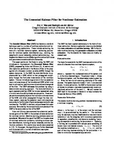
Table I TABLE OF THE RMS VALUES OF THE ESTIMATION ERROR FOR SEVERAL PARTICLE F ILTER VARIANTS Filter PF-SIR APF √ APF√ APF- 3 2 APF-MR √ APF-MR√ APF-MR- 3 2 UPF UPF - α = 0.1 UPF - α = 0.2 UPF - α = 1 UPF - α = 0
Mean Value
Standard Deviation
Maximum Value
5.41541 5.37662 5.31901 5.33066 5.33339 5.18590 5.19944 5.90033 5.08705 5.03754 5.12051 5.02658
1.34547 1.18517 1.13784 1.13710 1.16558 1.11002 1.13456 1.78609 1.37431 1.27727 1.27182 1.20974
11.63975 9.68630 9.32619 9.33985 9.42745 9.24750 9.58607 13.34652 13.44550 12.69427 12.59017 12.95750
determined experimentally. In any case, the choice α = 1 is also expected to give good enough results, especially if the convergence is fast enough. It is also possible to set the matrices Pki equal to 0, which is equivalent to α = 0. This choice has the advantage that in this case, the prediction step of the Unscented Kalman Filter is done with no computational cost, with the a priori mean equal to f (xik−1 ) and the a priori covariance matrix equal to the covariance matrix of the disturbance. The computational cost reduction gives the possibility to deploy a greater number of particles, in which case the term NPp will be even closer to 0. The proposed modifications are tested in a numerical example in the following section. V. N UMERICAL E XAMPLE AND C OMMENTS The system to which the different variants of the Particle Filter will be applied for comparison purposes is described by xk xk xk+1 = + 25 + 8 cos(1.2k) + wk , (19) 2 1 + x2k x2 yk = k + vk (20) 20 and appeared for the first time in [31]. Since, it has been extensively studied in the literature [17]–[20]. x0 , wk and vk are independent r.v. following the Gaussian distribution with zero mean. x0 has a covariance equal to 0.001 while, as in [17], [19], [20], for the covariances of wk and vk it is assumed that V [wk ] = 10, V [vk ] = 1. The system is run up to k = 100. 1000 repetitions have been performed and the results are presented in Table I. PF-SIR is the Sampling Importance Resampling Filter of the literature [19]. APF is the Auxiliary Particle Filter, for all whose variants the auxiliary weights are i computed for a random realization of the r.v. f (xik−1 )+wk−1 , √ √ 2 and 3 denote the proposed in Section III as in [19]. modifications in the way that the auxiliary weight is taken into account, while MR (Modified Reweighting) denotes the 2 See
the penultimate paragraph of this section.
Comp. Time
2
(ms)
0.18850 (3.56) 0.24240 0.24800 0.31380 0.28180 0.28530 0.35500 20.90770 20.91310 20.90010 20.90210 12.98660
proposed modification in the redetermination of the weights after resampling. UPF is the Unscented Particle Filter, and α is the parameter referred in Section IV. The resampling is performed using the algorithm proposed in [18], while as in the software [32], a very small value is added to the likelihoods so as to exclude the event that they are all 0 due to rounding. In all variants 50 particles have been used. It is concluded that the proposed modifications to the APF improve its performance, both if applied separately as well as if applied in combination, in which latter case the best results are obtained. Concerning the proposed modification to the UPF, among the various values of α tested, the best results were for α = 0, choice which, as already mentioned, has also a computational advantage. An interesting fact is that while UPF can, with proper adjustment, yield a small error in the mean case, in the worst case its error is greater even than that of PF-SIR. The computational costs of the various proposed techniques are different, but for PF and the variants of APF the differences are not big, as the differences among the variants of UPF. However the MATLAB implementation which has been made leads to high cost for UPF, because the computations in this case are not made “vectorized”. This has been made because using MATLAB it is easy to compute, for example, all the particle weights simultaneously, or to create all new particles using one function call, while the Unscented Kalman Filter equations were applied separately to each particle in the implementation made. If the particle computations for PF-SIR are also made non-vectorized, the cost is that appearing in parenthesis in Table I. The conclusion from the numerical results is that the proposed modification can reduce the estimation error, and the choice of the variant that will be used can be made taking into account the performance of the various variants in the problem under study as well as the technical details of the implementation that will be made. ACKNOWLEDGMENTS Alexandros Charalampidis wishes to thank the Special Account of Research of the National Technical University
7045
of Athens for supporting his doctoral research on Estimation Theory. The research of George P. Papavassilopoulos has been co-financed by the European Union (European Social Fund – ESF) and Greek national funds through the Operational Program “Education and Lifelong Learning” of the National Strategic Reference Framework (NSRF) - Research Funding Program: THALES, Investing in knowledge society through the European Social Fund. Support has been also provided by the program ARISTEIA, project HEPHAISTOS. R EFERENCES [1] Kalman, R. E.: A new approach to linear filtering and prediction problem. ASME Journal of Basic Engineering, 82(1):35–45, Mar. 1960. [2] Anderson, B. D. O. and J. B. Moore: Optimal Filtering. Prentice-Hall, Englewood Cliffs, NJ, 1979. [3] Goodwin, G. C. and K. S. Sin: Adaptive Filtering Prediction and Control. Dover Publications, New York, NY, USA, 2009. [4] Simon, D.: Optimal State Estimation: Kalman, H∞ and Nonlinear Approaches. John Wiley, Hoboken, NJ, 2006. [5] Kalman, R. E. and R. S. Bucy: New Results in Linear Filtering and Prediction Theory. Journal of Basic Engineering, 83D:95–108, 1961. [6] Smith, G. L., S. F. Schmidt, and L. A. McGee: Application of statistical filter theory to the optimal estimation of position and velocity on board a circumlunar vehicle. Technical Report TR R-135, NASA, 1962. [7] Julier, S., J. K. Uhlmann, and H. F. Durrant-Whyte: A New Method for the Nonlinear Transformation of Means and Covariances in Filters and Estimators. IEEE Transactions on Automatic Control, 45(3):477–482, Mar. 2000. [8] Julier, S. and J. K. Uhlmann: Unscented filtering and nonlinear estimation. Proceedings of the IEEE, 92(3):401–422, Mar. 2004. [9] Lefebvre, T., H. Bruyninckx, and J. d. Schutter: Kalman filters for nonlinear systems: a comparison of performance. International Journal of Control, 77(7):639–653, May 2004. [10] Simandl, Miroslav and Jindrich Dun´ık: Derivative-free estimation methods: New results and performance analysis. Automatica, 45(7):1749–1757, July 2009, ISSN 0005-1098. [11] Arasaratnam, I. and S. Haykin: Cubature Kalman Filters. Automatic Control, IEEE Transactions on, 54(6):1254–1269, June 2009, ISSN 0018-9286. [12] M. St-Pierre and D. Gingras: Comparison between the unscented Kalman filter and the extended Kalman filter for the position estimation module of an integrated navigation information system. In Proc. 2004 IEEE Intelligent Vehicles Symposium, pages 831–835, Jun. 2004. [13] Charalampidis, A. C. and G. P. Papavassilopoulos: Computationally Efficient Kalman Filtering for a Class of Nonlinear Systems. IEEE Transactions on Automatic Control, 56(3):483–491, Mar. 2011. [14] Charalampidis, A. C. and G. P. Papavassilopoulos: Kalman Filtering for a Generalized Class of Nonlinear Systems and a New Gaussian Quadrature Technique. IEEE Transactions on Automatic Control, 57(11):2967–2973, Nov. 2012. [15] Charalampidis, A. C. and G. P. Papavassilopoulos: Development and Numerical Investigation of New Nonlinear Kalman Filter Variants. IET Control Theory and Applications, 5(10):1155–1166, 2011. [16] Sorenson, H. W. and D. L. Alspach: Recursive Bayesian estimation using Gaussian sums. Automatica, 7(4):465–479, 1971. [17] Gordon, N. J., D. J. Salmond, and A. F. M. Smith: Novel approach to nonlinear/non-Gaussian state estimation. IEE ProceedingsF, 140(2):107–113, Apr. 1993. [18] Kitagawa, G.: Monte Carlo Filter and Smoother for Non-Gaussian Nonlinear State Space Modules. Journal of Computational and Graphical Statistics, 5(1):1–25, Mar. 1996. [19] Sanjeev Arulampalam, M., S. Maskel, N. Gordon, and T. Clapp: A Tutorial on Particle Filters for Online Nonlinear/Non-Gaussian Bayesian Tracking. IEEE Transactions on Signal Processing, 50(2):174–188, Feb. 2002. [20] Capp´e, O., S. J. Godsill, and E. Moulines: An overview of existing methods and recent advances in sequential Monte Carlo. Proceedings of the IEEE, 95(5):899–924, 2007.
[21] Pitt, M. K. and N. Shephard: Filtering via simulation: Auxiliary particle filters. Journal of the American Statistical Association, 94(446):590–599, June 1999. [22] van der Merwe, R., A. Doucet, N. de Freitas, and E. Wan: The Unscented Particle Filter. Technical Report CUED/F-INFENF/TR 380, Cambridge University, Aug. 2000. [23] Bayes, T.: An Essay towards solving a Problem in the Doctrine of Chances. Philosophical Transactions of the Royal Society of London, 53:370–418, 1763. [24] Billingsley, P.: Probability and Measure. Wiley-Interscience, Hoboken, NJ, 3rd edition, 1995. [25] Ash, R. B.: Basic Probability Theory. Dove, Mineola, NY, 2008. Available: www.math.uiuc.edu/∼r-ash/BPT.html. [26] Sorenson, H. W. and A. R. Stubberud: Non-linear filtering by approximation of the a posteriori density. International Journal of Control, 8(1):33–51, 1968. [27] Crisan, D. and A. Doucet: A survey of convergence results on particle filtering methods for practitioners. IEEE Transactions on Signal Processing, 50(3):736–746, Mar. 2002. [28] Hu, X. L., T. B. Schon, and L. Ljung: A Basic Convergence Result for Particle Filtering. IEEE Transactions on Signal Processing, 56(4):1337–1348, Apr. 2008. [29] Capp´e, Olivier: An Introduction to Sequential Monte Carlo for Filtering and Smoothing. http://www-irma.u-strasbg.fr/∼guillou/meeting/ cappe.pdf. [30] Orhan, Emin: Particle Filtering. http://www.bcs.rochester.edu/people/ eorhan/notes/particle-filtering.pdf. [31] Netto, M., L. Gimeno, and M. Mendes: On the optimal and suboptimal nonlinear filtering problem for discrete-time systems. Automatic Control, IEEE Transactions on, 23(6):1062–1067, Dec. 1978, ISSN 00189286. [32] de Freitas, N. and R. van der Merwe: http://www.cs.ubc.ca/∼nando/software/upf demos.tar.gz, Aug. 2000. MATLAB Code.
7046