Improved bounds for the symmetric rendezvous value on the line Qiaoming Han∗
Donglei Du†
Abstract A notorious open problem in the field of rendezvous search is to decide the rendezvous value of the symmetric rendezvous search problem on the line, when the initial distance apart between the two players is 2. We show that the symmetric rendezvous value is within the interval (4.1520, 4.2574), which considerably improves the previous best known result (3.9546, 4.3931). To achieve the improved bounds, we call upon results from absorbing markov chain theory and mathematical programming theory—particularly fractional quadratic programming and semidefinite programming. Moreover, we also establish some important properties of this problem, which may be of independent interest and useful for resolving this problem completely. Finally, we conjecture that the symmetric rendezvous value is asymptotically equal to 4.25 based on our numerical calculations.
1
Introduction
Consider two players situated on an (undirected) line who know their initial distance apart at time 0, but not the direction to the other player. Assume they move at a maximum speed of one. They obviously have no common sense of direction along the line because of the undirectness of the line. So we assume that Nature (or chance) assigns each player independently a random direction to call ‘forward’. A pure strategy for a player is simply a continuous path that describes her position relative to her starting point, in the direction she calls ‘forward’. The rendezvous search problem on the line involves prescribing strategies for both players to meet in least expected time, called the rendezvous value. We say that two players meet, or rendezvous occurs, if they ∗ School of Engineering and Management, Nanjing University. This work was done while the author was visiting the Faculty of Business Administration, University of New Brunswick. Supported in part by NSERC grants awarded to D. Du (283103) and Luis F. Zuluaga (290377), and NNSF grant of China. (
[email protected]) † Faculty of Business Administration, University of New Brunswick. Supported in part by NSERC grant 283103 and URF, FDF at UNB. (
[email protected]) ‡ Mellon College of Science, Carnegie Mellon University.
[email protected] § Faculty of Business Administration, University of New Brunswick. Supported in part by NSERC grant 290377 and FDF, UNB. (
[email protected])
Juan Vera‡
Luis F. Zuluaga§
occupy the same location on the line. There are two versions of the problem depending on whether the same strategy must be employed by both players or not. In the asymmetric rendezvous search problem, they could use distinct mixed or pure strategies. In the symmetric rendezvous search problem, they must choose the same mixed strategy. Note that no pure strategy can achieve a finite meeting time for the symmetric problem because of the lack of direction for both players—for example, if they both adopt the same pure strategy and initially face in the same direction, they will move in the same direction forever and never meet. Therefore mixed strategies must be employed in the symmetric problem. We consider here only the symmetric problem. Throughout this paper, we assume that the two players’ initial distance apart is 2 unless stated otherwise. Let Rs and Ra be the rendezvous values for the symmetric and asymmetric problems, respectively. Evidently Rs ≥ Ra because both players could always choose to adopt the same mixed strategy. Alpern and Gal [8] show that the asymmetric rendezvous value Ra = 3.25, and hence completely settle the asymmetric case. On the other hand, a notorious open problem, initially posed by Alpern [1] in 1995, is to decide the symmetric rendezvous value Rs . This open question is arguably the most important open one in rendezvous search theory [2, 9]. The symmetric rendezvous problem itself subjectively belongs to the category of P´olya: “the simplest problem one cannot solve” [17]. Besides its theoretical significance, such kind of rendezvous search problem also has practical applications in communication synchronization, operating system design, operations research, search and rescue operations planning, military, radio, and media press. For example, the military has always had protocols for rendezvous in unfamiliar territory, and the same goes for explorers. A particular example which could lead to the rendezvous search problem considered here is the situation where two parachutists landing in an unknown field want to meet as soon as possible. For detailed discussion of rendezvous search problems and their applications, please refer to the survey paper by Alpern [2] and the book by Alpern and Gal [9]. Alpern [1] introduces the symmetric rendezvous
Upper Lower search problem on the line and proposes a strategy with bound bound expected meeting time of 5. The idea is to repeat the Alpern [1] 5.0000 following moving pattern every 3 time units until renAlpern and Gal [8] 3.25 dezvous occurs: pick a random direction and move one Anderson and Essegaier [7] 4.5678 time unit in this direction and two time units in the Baston [11] 4.4182 opposite direction, all at speed one. Note that this kind Uthaisombut [19] 4.3931 3.9546 of strategy is very special in that both players adopt the same moving pattern. Anderson and Essegaier [7] Table 1: Previous upper and lower bounds for Rs improve the upper bound to 4.5678 by repeating, every 6 time units, a mixed movement over four moving patterns with prespecified probabilities. Anderson and EsIn the following, we summarize the main contribusegaier’s idea is innovative because mixed movements tions of this work and also briefly explain the main ideas provide the opportunity for the two players to actually and steps that lead to them. follow different moving patterns. This philosophy will 1. We show, in Theorem 2.1, that strategies that albe pushed further in this work to derive our bounds— ways move at maximum speed one and switch diboth upper and lower bounds. Baston [11] further imrection only at integer times (called grid strategies proves the upper bound to 4.4182 by repeating, every 7 in this paper) dominate among all possible stratetime units, a mixed movement over four patterns. This gies. To the best knowledge of the authors, this improvement is a result of the new observation that acseems to be unknown in the literature—but see a cumulated information before rendezvous should be utisimilar result by Lim et al. [15] in a different conlized in Anderson and Essegaier’s strategy. Uthaisom1 text. This greatly reduces the searching strategy but [19] recently presented a new mixed strategy with space of the problem. the previous best known upper bound of 4.3931. This strategy goes further to allow the mixture of patterns 2. To obtain better upper bounds, we investigate the with different time units, namely 6 and 7. aforementioned Markovian type strategies; that Note that all the previous strategies share the same is, the same mixed moving patterns are repeated spirit; namely that the same movement or mixed moveevery fixed time units before rendezvous occurs. ment is repeated over and over again until rendezvous For Markovian type strategies to perform well, occurs. This kind of strategy naturally induces a there are two opposite driving forces involved. On Markov chain if we define its state space as half of the the one hand, adding more moving patterns in distance apart after each repetition. Our upper bounds every repetition should reduce the symmetry of the will be also achieved by such Markovian type strategies, problem (or equivalently increase the asymmetry, but in a more systematic way. namely, increase the chance for two players to adopt In terms of lower bounds, there are fewer results. different pure strategies), and hence increase the a Besides the obvious lower bound R , the previous best meeting opportunity. This necessitates increasing known lower bound of 3.9546 is recently given also the length of the moving patterns. On the other by Uthaisombut [19]. The lower bound scheme of hand, with longer length, the expected time to Uthaisombut is based on the simple observation that meet also increases, mainly because there is at if two players are a distance d apart, then the expected least 1/2 probability for the two players to move in extra time to meet is at least d/2. the same direction whenever they adopt the same s Previous existing lower and upper bounds on R are moving pattern and hence will never meet within summarized in Table 1 below. one repetition. Therefore, the main challenge is how to balance these two forces. We manage to quantify this balance; that is, the expected time of any strategy can be expressed as the product of two inversely related expectations: one local and one global. See Section 3.1 for more details.
1 This recent work was brought to our attention after the current work was almost done.
(a) First, in Theorem 2.2, we show that distancepreserving Markovian type strategies dominate, which implies the aforementioned balancing relationship and further reduces the searching space. The essential idea behind
this result is that when using a non-distancepreserving Markovian type strategy, once the distance of the two players increase to certain point it will follow a symmetric random walk and therefore the expected time to reduce such distance is infinite—a well-know result in random walk theory. (b) Next, we reduce the performance analysis of Markovian type strategies to solving a fractional quadratic program whose value for any feasible solution provides an upper bound for Rs . This allows us to utilize the Mathematical Programming (MP) toolkit, particularly Quadratic Programming (QP) and Semidefinite Programming (SDP). 3. To obtain better lower bounds, we consider a related problem first introduced by Alpern and Gal [10], the symmetric rendezvous search on a directed line, whose only difference with the original problem is that both players are given the direction of the line and hence the rendezvous value RU for the new problem provides a lower bound for the original one because of the new information given. In the new problem, we employ the observation that if two players have been following the same strategy (and hence in the same direction for certain time), then no information has been acquired and both players are facing exactly the same situation as started initially. Therefore the expected extra time to meet is still RU . The new insight leads to solving a different fractional quadratic program whose optimal value provides a lower bound for Rs ≥ RU . See Section 3.2 for more details. 4. Based on the ideas above, we show that the symmetric rendezvous value is within the interval (4.1520, 4.2574). 5. Finally, based on our numerical calculations, we conjecture that the symmetric rendezvous value is equal to 4.25, which can only be achieved asymptotically by the procedure n-Markovian, introduced in Section 2.2. This value is only asymptotically achievable because our calculation indicates that increasing the length of the moving patterns is the dominating force among the two discussed in (2). See Section 4 for more details. The rest of the paper is organized as follows. We first prove the two domination results in Sections 2.1 and 2.2. We then present the improved upper and lower bounds in Sections 3.1 and 3.2, respectively. Finally we give some concluding remarks in Section 4.
2
Strategies
In the symmetric rendezvous search problem on the (undirected) line, two players, I and II, are situated initially at a known distance 2 apart on a line and wish to meet in least expected time, given that they both move at a maximum speed of 1. They are told the initial distance apart, but neither the direction to the other player nor the direction along the line. So we assume that Nature (or chance) assigns each player independently a random direction to call ’forward’. A pure strategy for a player is simply a Lipshitz continuous path with maximum speed one that describes her position relative to her starting point, in the direction she calls ’forward’. Therefore the set of all pure strategies is given by S
= {s : R+ → R, s(0) = 0, |s(t1 ) − s(t2 )| ≤ |t1 − t2 |, ∀t1 , t2 ∈ R+ }.
A mixed strategy x over the pure strategy space S is a Borel probability measure over S. The set of all mixed strategies over S will be denoted as S ∗ . Given two pure strategies s1 , s2 ∈ S, there are four equally likely meeting times, depending on the four situations in which Nature initially faces the players and the relative positions of the players, namely: towards or away from each other, same direction with player I or II in front. Let T (s1 , s2 ) denote the meting time of the players whenever they adopt pure strategies s1 and s2 , respectively. Consequently, T (s1 , s2 ) is a (discrete) random variable whose probability distribution can be identified by considering all four equally likely possibilities above. For computational purposes, assume that player I is placed at point 0 and player II at point 2 at time 0. Then: 1. Player I follows path 0 + s1 (t) and Player II follows path 2 + s2 (t). The probability is 1/4 with meeting time t++ (s1 , s2 ) = min{t : s1 (t) = 2 + s2 (t)}. 2. Player I follows path 0 − s1 (t) and Player II moves toward 2 − s2 (t). The probability is 1/4 with meeting time t−− (s1 , s2 ) = min{t : 0 − s1 (t) = 2 − s2 (t)}. 3. Player I follows path 0 + s1 (t) and Player II follows path 2 − s2 (t). The probability is 1/4 with meeting time t+− (s1 , s2 ) = min{t : 0 + s1 (t) = 2 − s2 (t)}.
4. Player I follows path 0 − s1 (t) and Player II follows path 2 + s2 (t). The probability is 1/4 with meeting time t−+ (s1 , s2 ) = min{t : 0 − s1 (t) = 2 + s2 (t)}. So the expected meeting time t(s1 , s2 ) is given by t(s1 , s2 ) = E[T (s1 , s2 )] =
1 X δ1 δ2 (s1 , s2 ), t 4 δ1 ,δ2
Figure 1a: Proof of Theorem 2.1
where δ1 , δ2 ∈ {+, −}. Similarly for any two mixed strategies x1 , x2 ∈ S ∗ , we define their expected meeting time, or rendezvous time, by t(x1 , x2 ) = Ex1 ,x2 [t(s1 , s2 )]. The asymmetric and symmetric rendezvous values Ra and Rs are defined respectively as
(2.1)
Ra
=
Rs
=
min t(x1 , x2 );
x1 ,x2
min t(x, x).
Figure 1b: Proof of Theorem 2.1
x
The symmetric rendezvous problem therefore is to find an optimal strategy for both players with minimum Rs , that is, to solve the optimization problem (2.1). As a convention throughout this paper, any set ⋆ with an asterisk (∗ ) attached—that is ⋆∗ —is the set of mixed strategies over the given set. For example, S ∗ is the set of mixed strategies over S. 2.1 Grid Strategies A strategy s ∈ S is grid if the speed at every instant is one and direction can only be switched at integer times. Denote SG to be the ∗ set of all grid strategies, and hence SG is the set of all mixed strategies over SG according to our convention. We want to prove that we can reduce the problem to ∗ searching only mixed grid strategies SG . This result follows evidently from the result below.
Figure 1c: Proof of Theorem 2.1
Theorem 2.1. There is b· : S → SG such that for every pair of pure strategies s1 , s2 ∈ S t(s1 , s2 ) ≥ t(b s1 , sb2 ).
Proof. First we define b· : S → SG . Fix s ∈ S. Consider the curve C(t) = (s(t), √ t) ∈ IR × IR+ and the ”diagonal” grid with side length 2 (Figure 1a). Shadow every square that C crosses. In case the curve C goes through a corner from one square to a diagonally adjacent one above, shadow also the left one of the two squares adjacent to both squares (Figure 1b). Mark the lowest b be corner of each shadowed square (Figure 1c). Let C
Figure 1d: Proof of Theorem 2.1 the piecewise linear curve obtained by joining adjacent b marked corners and let sb such that C(t) = (b s(t), t) (Figure 1d). Now given s1 , s2 ∈ S we need to show t(s1 , s2 ) ≥ t(b s1 , sb2 ). It suffices to show that tδ1 δ2 (s1 , s2 ) ≥ δ1 δ2 (b s1 , sb2 ) for every δ1 , δ2 ∈ {+, −}. If tδ1 δ2 (s1 , s2 ) = t ∞ there is nothing to prove. So let t0 = tδ1 δ2 (s1 , s2 ),
Figure 1e: Proof of Theorem 2.1 and let x0 := δ1 s1 (t0 ) = δ2 s2 (t0 ) + 2. The paths δ1 s1 and δ2 s2 + 2 meet at the point (x0 , t0 ). Let S0 be the grid square containing (x0 , t0 ) and let (x1 , t1 ) be the lowest corner of S. By construction the two curves \ (δ1 sb1 , t) = (δd 1 s1 , t) and (δ2 sb2 + 2, t) = (δ2 s2 + 2, t) meet at (x1 , t1 ). Thus δ1 sb1 (t1 ) = δ2 sb2 (t1 ) + 2 and therefore t(δ1 sb1 , δ2 sb2 ) ≤ t1 ≤ t (Figure 1e).
2.2 Distance-preserving strategies From now on we will only consider the grid strategy space SG . We introduce the notion of string over the alphabet set {−1, 1} such that the first element of any string is 1, referring to a ’forward’ movement of one time unit chosen by the Nature initially; and each other element 1 corresponds to the same ’forward’ movement of one time unit and each -1 corresponds to the ’backward’ movement of one time unit, all at speed one. Obviously any grid strategy can be equivalently viewed as such a string of infinite length. To facilitate our analysis, we call a string of finite length n, a positive integer, an n-generator. For example, the 3-generator g = {1, −1, −1} means moving 1 time unit in the ’forward’ direction and 2 time units in the other, all at speed one. The set of all n-generators will be denoted as Gn . Evidently the cardinality of Gn is 2n−1 . A mixed n-generator x ∈ Gn∗ is a Borel probability measure x over the set Gn . Denote Ik = {1, 2, · · · , k} as an index set for any given positive integer k. Any vector will be a column vector. A vector x = (xi )i∈Ik is a probability vector if it satisfies xi ≥ 0, ∀i ∈ Ik and eT x = 1, where e is the vector of all ones. Fix a positive integer n. Given a mixed n-generator x ∈ Gn∗ , we prescribe the following (mixed) strategy followed by both players, which will be used to derive our upper bound: n-Markovian: Repeat the mixed n-generator x every n time units until rendezvous occurs.
ther becomes zero or remains unchanged after one player follows g1 and another player follows g2 for n time units. ∗ A mixed n-generator x ∈ SG is distance-preserving if xi xj = 0 whenever gi ≁ gj for all i, j ∈ I2n−1 . We shall show in this section that distancepreserving mixed generators dominate among all mixed strategies in Gn∗ for strategy n-Markovian. Actually we shall prove a stronger result that no non-distancepreserving mixed n-generator used in n-Markovian can guarantee finite expected meeting time. Theorem 2.2. For any given positive integer n, the expected meeting time of strategy n-Markovian is infinite whenever the mixed n-generator used in strategy n-Markovian is non-distance-preserving. Proof. Let dt be the distance of the two players after t repetitions (of n time units each) of the n-Markovian strategy. Let x ∈ Gn∗ be a non-distance preserving mixed n-generator. Let p = Prg1 ,g2 ∈Gn [g1 6∼ g2 ], i.e. p is the probability that the distance will actually increase when starting at distance 2 and using x as the mixed generator for the n-Markovian strategy, and by assumption p > 0. Given g1 , g2 ∈ Gn and δ1 , δ2 ∈ {+, −} assume that dt > 2n and that at time t the two players follow g1δ1 and g2δ2 , respectively. As dt > 2n the two paths cannot cross and therefore dt+1 = dt + δ1 s(g1 ) − δ2 s(g2 ),
Pn where for every g ∈ Gn we define s(g) = i=1 gi . For i = −n, Pn. . . , n, let pi = Pr [dt+1 − dt = 2i|dt > 2n]. We have i=−n pi = 1 and by the symmetry of the strategy p−i = pi . Now let X0 = 0 and let Xt be defined for every t = 0, 1, 2, . . . by Xt+1 = Xt + i with probability pi , i = −n, . . . , n. Let T be the first t when Xt < 0. Conditional in dn > 2n we can couple the construction of Xt and the process n-Markovian such that dt+n > 2Xt + 2n for all t = 0, 1, . . . , T . As Pr [dn > 2n] ≥ pn and to get dt = 0, we must first get dt ≤ 2n implying Xt < 0. We have then the expected meeting time for n-Markovian is at least pn (n + E[T ]). But Xt is a symmetric random walk starting at 0 and therefore E[T ] = ∞, a well-known result of the random walk theory [13]. 3
Bounding the symmetric rendezvous value Rs
3.1 Upper bound We will analyze the performance of the mixed strategy n-Markovian. Because of TheTwo n-generators g1 , g2 ∈ Gn are distance- orem 2.2, we only need to focus on distance-preserving preserving, denoted as g1 ∼ g2 , if their distance apart ei- mixed generators in n-Markovian.
Let x ∈ Gn∗ be a distance-preserving mixed n- (3.2) can also be derived based on results from absorbgenerator used in n-Markovian such that Gn = ing Markovian chain theory where the state space con{g1 , · · · , g2n−1 } and x = (x1 , · · · , x2n−1 ). sists of only states 0 and 1 when restricted to distancepreserving strategies. Note that the numerator above can Remark 3.1. We note that computational efficacy can be viewed as the expected ”effective” meeting time, the be achieved if we reduce the cardinality of Gn by ex- time they spend within each state of the aforementioned cluding any generator that is non-distance-preserving Markov chain (the local factor), and the denominator with itself. For example we can exclude the generator is the probability that the two players will meet after {1, 1, · · · , 1} because it does not preserve distance with time n, whose reciprocal is the expected absorbing time itself. This proves to be extremely beneficial in calcu- of the Markov chain (the global factor). Therefore the lating upper bounds for Rs numerically. This is im- last equation is actually equal to the product of two inplemented in our numerical calculation. However, this versely related expectations: one local and one global. reduction is equivalent to setting zeros to the probabil- This quantifies the balancing idea mentioned in the inities of those excluded generators when computational troduction. efficacy is not an issue. Therefore we will assume the cardinality of Gn is still 2n−1 for simplicity of presentaSo the objective value of any feasible solution to tion. the following fractional quadratic programming problem Consider two n-generator gi , gj ∈ Gn such that one provides an upper bound for the symmetric rendezvous s player follows gi and another follows gj for n time units. value R : ½ T x Mn x • Let pij be the probability that their distance apart (3.3) Rs = min : xi xj = 0, n 1 − xT Pn x at time n remains unchanged, given that they have ª not met by then. ∀gi ≁ gj , i, j ∈ I2n−1 , eT x = 1, x ≥ 0 . (n)
= For any fixed n, the tightest upper bound is the optimal • Let Tij be their meeting time. Let Tij min{Tij , n}, whose probability distribution follows value Rs . However, finding Rs for this particular n n (n) from that of Tij . Let mij = E[Tij ]. fractional quadratic program is hard when n is large. We obtain the following upper bounds of Rs for n ≤ 15. n−1 n−1 Denote matrix Pn = (pij ) ∈ R2 ×2 and matrix n−1 n−1 Mn = (mij ) ∈ R2 ×2 . Let T (x) be the expected n Rns Achieved No. of Strategies meeting time of the mixed strategy n-Markovian, 1 ∞∗ 1 using x as the mixed n-generator. Then it is easy to 2 7.0000∗ 1 verify the following: 3 5.0000∗ 1 4 4.9441∗ 2 T T T (x) = x Mn x + T (x)x Pn x, 5 4.8827∗ 4 6 4.4634∗ 5 where xi xj = 0 whenever gi ≁ gj , , i, j ∈ I2n−1 . Or 7 4.3490∗ 5 equivalently, 8 4.3209∗ 8 xT Mn x 9 4.3044∗ 11 . (3.2) T (x) = 10 4.2866 18 1 − xT Pn x 11 4.2739 29 Remark 3.2. The n-Markovian strategy can also be 12 4.2678 38 interpreted via absorbing Markovian chain theory. For 13 4.2630 58 mixed strategy n-Markovian, we associate an absorb14 4.2595 89 ing Markov chain with state space M = {0, 1, 2, · · · } 15 4.2574 128 and transition probability matrix Q = (qij ). Each state .. .. .. . . . i ∈ M corresponds to half of the distance apart after
∞ 4.25? ∞? every n time units. Therefore each qij gives the conditional probability that half of the distance apart switches Table 2: Upper bounds for Rs from i to j, for i, j ∈ M. State 0 is absorbing, and the rest is transient. Theorem 2.2 basically says that Matlab code for solvthe expected absorbing time starting from state 1 is in- Remark 3.3. The (3.3) can be downloaded from our finite whenever a non-distancing-preserving mixed gen- ing However we erator is used in n-Markovian. Therefore the formula website,”http://www.unb.ca/∼ ddu”.
note that the codes therein do not directly solve (3.3). precision 10−5 ) prove the fact above except for the To be more computationally efficient, we reduce the simple cases of n = 1, 2 and 3, whose optimality can be search space using the idea introduced in Remark showed easily by first-hand analysis. 3.1. Moreover, to obtain the bounds listed in Table 2 • R1s = ∞: In this case there is just one generator using nonlinear optimization solvers, one may need to g = {1}, which is non-distance-preserving and choose an appropriate initial feasible solution to start hence R1s = ∞ based on Theorem 2.2. with (a notorious feature of nonlinear programming). More details on the implementation are included in • R2s = 7: In this case, there are two generators: the self-contained explanation within the Matlab code g1 = {1, −1}, g2 = {1, 1}. But g1 is the only files on our website. Finally, we only retain four digits distance-preserving generator with R2s = 7. This after the decimal point for the upper bounds in Table can be easily verified by substituting M2 = 1(1/4)+ 2. More digits can be obtained by running the Matlab 2(3/4) = 7/4 and P2 = 3/4 into (3.3). code under long format environment (up to 10−16 with • R3s = 5: In this case, there are four generators: double precision). g1 = {1, 1, 1}, g2 = {1, 1, −1}, g3 = {1, −1, 1}, g4 = {1, −1, −1}. But g4 is the only distance-preserving Some of the bounds given in Table 2 are actually generator with R3s = 5. This can be easily verified best possible (indicated with an *) for fixed n up to by substituting M3 = 1(1/4) + 3(1/4) + 3(1/2) = computation precision. Note that, although the entries 5/2 and P3 = 1/2 into (3.3). This is Alpern’s in matrices Mn and Pn are calculated exactly, we can strategy [1]. only prove a solution is best possible up to computation precision. In the following, we only retain four digits after the Fact 3.1. The Rns listed in Table 2 is the optimal value decimal point for each value. Again, more digits can be of the fractional quadratic program (3.3) (hence the best obtained by running the Matlab code under long format environment as explained in Remark 3.3. rendezvous value) for any fixed integer n ≤ 9. • R4s ≈ 4.9441: The optimal mixed 4-generator is We prove this fact by considering each fixed n ≤ 9. given below. It suffices to show that each value is indeed the optimal one for the fractional quadratic program (3.3). We need the following result that relates fractional quadratic program to regular quadratic program. For any r > 0, define © (3.4) f (r) = min xT (Mn + rPn ) x : xi xj = 0, ª ∀gi ≁ gj , i, j ∈ I2n−1 , eT x = 1, x ≥ 0 . Lemma 3.1. If f (r∗ ) = r∗ in (3.4), then Rns = r∗ in (3.3).
So solving (3.3) reduces to searching for a fixed point of f , which involves solving a series of regular quadratic programs (3.4). Unfortunately, (3.4) in general is non-convex. To show that the solution obtained for (3.4) is indeed global, we also solve its SDP relaxation with SDP solvers SEDUMI [18] and DSDP5 [12]. © min (Mn + rPn ) • X : X • eeT = 1, Xij = 0, ∀gi ≁ gj , Xij ≥ 0, i, j ∈ I2n−1 , X º 0} , n−1
n−1
where X ∈ R2 ×2 and the operation • is the inner product of matrices by taking matrix as vectors. If there exists a feasible solution to (3.4) that achieves the optimal value of the SDP relaxation, then it must be a global optimal solution of (3.4). In the following, we adopt this idea to (numerically up to
g1 = {1,1,-1,-1}, g2 = {1,-1,-1,1},
x1 ≈ 0.1118 x2 ≈ 0.8882
• R5s ≈ 4.8827: The optimal 5-mixed generator is given below. g1 g2 g3 g4
= = = =
{1,-1,-1,-1, 1}, {1,-1,-1, 1,-1}, {1,-1, 1,-1,-1}, {1, 1,-1,-1,-1},
x1 x2 x3 x4
≈ ≈ ≈ ≈
0.3227 0.2500 0.1773 0.2500
• R6s ≈ 4.4634: The optimal 6-mixed generator is given below. g1 g2 g3 g4 g5
= = = = =
{1,-1,-1,-1,1,1}, {1,-1,-1,1,-1,1}, {1,-1,-1,1,1,-1}, {1,-1,1,-1,-1,-1}, {1,1,-1,-1,-1,-1},
x1 ≈ 0.2482 x2 ≈ 0.1561 x3 ≈ 0.1561 x4 ≈ 0.1867 ,x5 ≈ 0.2529
This result is a little bit better than the upper bound 4.5678 of Anderson and Essegaier [7], whose mixed 6-generator is given below. g1 g2 g3 g4
= = = =
{1,-1,-1,-1,1,1}, {1,-1,-1,1,-1,-1}, {1,-1,1,-1,-1,-1}, {1,1,-1,-1,-1,-1},
x1 x2 x3 x4
≈ ≈ ≈ ≈
0.4040 0.2120 0.1561 0.2279
• R7s ≈ 4.3489: The optimal mixed 7-generator is given below.
3.2 Lower bound We give a general framework for generating lower bounds. We need a new problem called the symmetric rendezvous problem on a directed line, g1 = {1,-1,-1,-1,1,1,1}, x1 ≈ 0.2617 first introduced by Alpern and Gal [10]. The difference g2 = {1,-1,-1,1,-1,1,-1}, x2 ≈ 0.1544 between this problem and the original symmetric reng3 = {1,-1,-1,1,1,-1,-1}, x3 ≈ 0.1544 dezvous problem on a (undirected) line is that in the new g4 = {1,-1,1,-1,-1,-1,1}, x4 ≈ 0.1940 problem the players have a common sense of direction. g5 = {1,1,-1,-1,-1,-1,-1}, x5 ≈ 0.2355 Along a similar proof line to Theorem 2.1, we can show This is better than the upper bound 4.4182 of that grid strategies still dominates in the new problem. Baston [11], whose mixed 7-generator is given So we will focus only on grid strategies. But the number of grid strategies is doubled compared to the original below. problem and it consists of all grid strategies, denoted as g1 = {1,-1,-1,-1,1,1,1}, x1 ≈ 0.2865 SU , generated by strings over the alphabet set {1, −1}, g2 = {1,-1,-1,1,1,-1,-1}, x2 ≈ 0.2471 not just those starting with 1. We denote RU to be the g3 = {1,-1,1,-1,-1,-1,1}, x3 ≈ 0.2139 symmetric rendezvous value of the new problem. Evig4 = {1,1,-1,-1,-1,-1,-1}, x4 ≈ 0.2524 dently, Rs ≥ RU because more information is available lower This is also better than the previous best upper (common direction) in the new problem. So any s bound on R will be a valid lower bound for R also. U bound 4.3931 of Uthaisombut[19], who mixes one Let x ∈ SU∗ be a given mixed strategy over SU . Fix 6-generator and four 7-generator’s. a positive integer n. Assume that Gn = {g1 , g2 , · · · , g2n } g1 = {1,1,-1,-1,-1,-1,-1}, is the set of n-generator’s. For any n-generator gi ∈ Gn g2 = {1,-1,1,-1,-1,-1,1}, (i ∈ I2n ), let Gn (gi ) ⊂ SG be the subset of strategies g3 = {1,-1,-1,1,-1,1,-1}, of SG that have R the same first n elements as gi . Define g4 = {1,-1,-1,1,-1,-1,1}, b = (b x1 , · · · , x b2n )T is a further x bi = Gn (gi ) dx. Then x g5 = {1,-1,-1,-1,1,1}. probability vector. So x b(Gn ) is a mixed n-generator over G . n • R8s ≈ 4.3208: The optimal mixed 8-generator is Let H(x) be the expected meeting time of the mixed given below. strategy x when the initial distance is 2. The following scheme is an improvement over that of Uthaisombut g1 = {1,-1,-1,-1,1,1,1,1}, x1 ≈ 0.2038 [19]. Below we adopt some notations from [19]. For g2 = {1,-1,-1,1,-1,1,-1,1}, x2 ≈ 0.0881 any given positive integer n, we construct the following g3 = {1,-1,-1,1,-1,1,1,-1}, x3 ≈ 0.0977 pseudo-strategy with expected meeting time at least as g4 = {1,-1,-1,1,1,-1,-1,-1}, x4 ≈ 0.1577 good as, H(x), that of x when the initial distance apart g5 = {1,-1,1,-1,-1,-1,1,1}, x5 ≈ 0.1220 is 2. g6 = {1,-1,1,-1,-1,1,-1,-1}, x6 ≈ 0.0945 g7 = {1,1,-1,-1,-1,-1,-1,1}, x7 ≈ 0.1296 Pseudo-strategyn : Follow x b first, and, if rendezvous g8 = {1,1,-1,-1,-1,-1,1,-1}, x8 ≈ 0.1066 has not occurred yet, then • R9s ≈ 4.3044: The optimal mixed 9-generator is Case 1. the two players move toward each other, given below. if they have not been following the same basic grid strategy, or they have been following the g1 = {1,-1,-1,-1, 1, 1,-1, 1, 1}, x1 ≈ 0.1150 same basic grid strategy and in the opposite g2 = {1,-1,-1,-1, 1, 1, 1,-1,-1}, x2 ≈ 0.1485 direction up to n; g3 = {1,-1,-1, 1,-1,-1, 1, 1, 1}, x3 ≈ 0.0831 g4 = {1,-1,-1, 1,-1, 1,-1,-1, 1}, x4 ≈ 0.0613 Case 2. the two players adopt the optimal mixed g5 = {1,-1,-1, 1,-1, 1,-1, 1,-1}, x5 ≈ 0.0577 strategy for the symmetric rendezvous search g6 = {1,-1,-1, 1, 1,-1,-1,-1,-1}, x6 ≈ 0.1160 problem, if they have been following the same g7 = {1,-1, 1,-1,-1,-1, 1,-1, 1}, x7 ≈ 0.0507 grid strategy and in the same direction up to g8 = {1,-1, 1,-1,-1,-1, 1, 1,-1}, x8 ≈ 0.0672 n. g9 = {1,-1, 1,-1,-1, 1,-1,-1,-1}, x9 ≈ 0.0634 g10 = {1, 1,-1,-1,-1,-1,-1, 1, 1}, x10 ≈ 0.1304 We need two simple facts before we can show that g11 = {1, 1,-1,-1,-1,-1, 1,-1,-1}, x11 ≈ 0.1067 the expected meeting time of the pseudo-strategy is no more than that of x. All other cases up to n = 15 can be downloaded from our website ”http://www.unb.ca/∼ ddu”. Fact 3.2. In Pseudo-strategyn , if two players are
d distance apart after following the mixed strategy x b for Proof. Note that we have the following formula for H: n time units, then X (RU ) (b xi )2 H(x) ≥ (b x)T MnU x b+ 1. the minimum expected extra time for them to meet i∈I2n ! Ã is at least d/2; X X (d) d x bi x bj + pij 2 n i,j∈I2
2. moreover, if they have been following the same grid strategy (and hence in the same direction up to n implying d = 2), then the minimum expected extra time for them to meet is RU .
Proof. The first claim is obvious [19]. We only prove the second. Suppose the two players have been following the same strategy and hence in the same direction up to n. Therefore they arrive at exactly the same situation as started initially. So the minimum expected extra time for them to meet is RU .
d∈D
(b x)T MnU x b + RU (b x)T x b ¶ µ X 1 E[dij ] x bi x bj + 2 i,j∈I2n µ ¶ 1 U T Mn + RU In + Dn x b. = (b x) 2 =
The inequality above follows from Fact 3.2 and the definition of dij ’s. This proves the lemma because the last quantity is exactly the expected meeting time of the Pseudo-strategyn .
∗ Let x∗ ∈ SG be an optimal mixed strategy for the symmetric rendezvous search problem with initial distance 2. So RU = H(x∗ ). Based on the lemma above, • If i 6= j, then let dij be the distance apart when we obtain the following relationship one player follows sbi and the another follows sbj ¶ for n time units, assuming initial distance 2. If ³ ´T µ 1 c∗ . c∗ RU = H(x∗ ) ≥ x MnU + RU In + Dn x i = j, then let dii be the distance apart when 2 both players follow sbi in the opposite direction for n time units, assuming initial distance 2. Obviously dij is a discrete random variable whose support So, set is D = {0, 2, · · · , 2(n + 1)} with corresponding ³ ´T ¡ ¢ (2(n+1)) (0) (2) c∗ c∗ x MnU + 21 Dn x . probabilities pij , pij , · · · , pij . RU ≥ ³ ´T c∗ x c∗ 1− x
We introduce more notations.
• Let Uij be their meeting time when one player follows sbi and the another follows sbj for n time units, assuming initial distance 2. Since both players have a common direction, Nature’s only choice is to place either I or II in front. So Uij is a discrete random variable with only two equi(n) probably supports. Let Uij = min{Uij , n}, whose probability distribution follows from that of Uij . (n) Let uij = E[Uij ].
c∗ is obviously a feasible solution of Note that x the the following fractional quadratic program (3.5). Therefore, the optimal value of this program is a valid lower bound of RU for any fixed n. So Rs ≥ RU ≥ rns . (3.5) ½ T ¾ x (MnU + 12 Dn )x T s rn = min : e x = 1, xi ≥ 0, i ∈ I2n . 1 − xT x
Similarly as the upper bound, solving this fractional quadratic program is equivalent to solving a series of regular quadratic programs, which are non-convex in general. Again, to guarantee the global optimality, we also solve the SDP relaxations of the regular quadratic programs. We manage to obtain the Lemma 3.2. The expected meeting time of the following lower bounds for n ≤ 7. The Matlab Pseudo-strategyn is no more than H(x), that of code for solving (3.5) can be downloaded from our ∗ x ∈ SG , assuming initial distance 2. website,”http://www.unb.ca/∼ ddu”. Denote the expected distance matrix Dn = (E[dij ]) ∈ n n n n R2 ×2 . Denote matrix MnU = (uij ) ∈ R2 ×2 . Let n n In ∈ R2 ×2 be the identity matrix.
n 1 2 3 4 5 6 7
rns 3 3.2970 3.5869 3.8141 3.9784 4.0913 4.1520
Uthaisombut [19] 2 2.5 3 3.4375 3.6458 3.8326 3.9546
Table 3: Lower bounds for Rs We note that the lower bound scheme of Uthaisombut [19] does not distinguish the two cases in Pseudostrategyn . Instead only the idea in Case 1 of Fact 3.2 is applied. To see the advantage of adding Case 2, we also quote the lower bounds obtained in [19] (last column of Table 3). 4 Concluding remarks First, we note that any result obtained in this work can be extended to an arbitrary initial deterministic distance d rather than just 2. For random d with bounded support, the upper bound can be extended. Moreover, we offer the following conjecture based on our numerical calculations. Conjecture: Rs = lim Rns = 4.25. That is, the n→∞ optimal mixed strategy is attained asymptotically by letting n → ∞ in n-Markovian. Finally, we address the computational limitations of our lower- and upper-bounding techniques. Due to computer memory limitation, we are able to find upper bounds only for n ≤ 15 and lower bounds only for n ≤ 7. The asymmetry here is because of two main reasons: (1) only a global optimizer is a valid lower bound while any local optimizer can serve as a valid upper bound; and (2) in the upper bound calculation, we only need to consider distance-preserving strategies, while in the lower bound calculation, we have to consider all strategies. The computational requirement becomes so extensive with n increasing, and parallel computing techniques should be adopted in order to get better numerical bounds for large n. However, we believe that proving the conjecture theoretically will be more desirable and challenging. 5
Acknowledgments
We are extremely grateful to Drs. S. Alpern and S. Gal [10] for pointing out an error in the lower bound argument in the original draft and suggesting the correction in the current revised version. We also thank one of the referees for encouraging us to find the shorter proof of Theorem 2.2 presented here.
References [1] S. Alpern, The rendezvous search problem. SIAM J Control Optimization, 33 (1995), 673-678. [2] S. Alpern, Rendezvous Search: A Personal Perspective, Operations Research, 50 (2002), 772-795. [3] S. Alpern and S. Beck, Rendezvous search problem on the line with bounded resources: Expected time minimization. Eur J Oper Res, 101 (1997), 588-597. [4] S. Alpern and S. Beck, Asymmetric rendezvous on the line is a double linear search problem. Math. Oper. Res. 24(3) (1999), 604-618. [5] S. Alpern and S. Beck, Rendezvous search on the line with bounded resources: Maximizing the probability of meeting. Oper. Res. 47(6) (1999), 849-861. [6] S. Alpern and S. Beck, Pure strategy asymmetric rendezvous on the line with an unknown initial distance. Oper. Res. 48(3) (2000), 1-4. [7] E. J. Anderson and S. Essegaier, Rendezvous search on the line with indistinguishable players. SIAM J Control Optim, 33 (1995), 1637-1642. [8] S. Alpern and S. Gal, The rendezvous search problem on the line with distinguished players. SIAM J Control Optim, 33 (1995), 1271-1277. [9] S. Alpern and S. Gal, The theory of search games and rendezvous. Kluwer Academic Publishers, 2003. [10] S. Alpern and S. Gal, private communication, 2006. [11] V.J. Baston, Two rendezvous search problems on the line, Naval Res Logist. 46 (1999), 335-340. [12] S. J. Benson and Y. Ye. DSDP5: Software for semidefinite programming. Technical Report ANL/MCSP12890905, Mathematics and Computer Science Division, Argonne National Laboratory, September 2005. http://www-unix.mcs.anl.gov/DSDP/. [13] W. Feller, An introduction to probability theory and its applications. Volume 1, Wiley, 1950, 307-344. [14] S. Gal, Rendezvous search on the line. Oper. Res. 47 (1999) 974-976. [15] W.S. Lim, A. Beck, and S. Alpern, Rendezvous search on the line with more than two players. Oper. Res. 45(3) (1997) 357-364. [16] C. D. Mayer, Matrix analysis and applied linear algebra, SIAM, 2000, 124. [17] G. P´ olya, How to solve it: a new aspect of mathematical method, 2nd Ed., Princeton University Press, Princeton NJ, 1957. [18] J. F. Sturm, Using SeDuMi 1.02, a matlab toolbox for optimization over symmetric cones. Optim. Methods and Softw. 11-12 (1999), 625-653. [19] P. Uthaisombut, Symmetric rendezvous search on the line using moving patterns with different lengths. Working paper, Department of Computer Science, University of Pittsburgh, 2006.