Improved CLP Scheduling with Task Intervals - Semantic Scholar

Improved CLP Scheduling with Task Intervals Yves Caseau Bellcore, 445 South Street, Morristown NJ 07960, USA. [email protected]

François Laburthe Ecole Normale Supérieure 45, rue d’Ulm, 75005 PARIS [email protected]

Abstract In this paper we present a new technique that can be used to improve performance of job scheduling with a constraint programming language. We show how, by focusing on some special sets of tasks, one can bring CLP in the same range of efficiency as traditional OR algorithms on a classical benchmark (MT10 [MT63]), thus making CLP both a flexible and an efficient technique for such combinatorial problems. We then present our programming methodology which we have successfully used on many problems, and draw conclusions on what features constraint programming languages should offer to allow its use.

1. Introduction Real-life scheduling problems are often the composition of various well-identified hard problems. In the previous years, we have worked on applications such as task-technician assignments [CK92] or staff timetable scheduling [CGL93] and developed a methodology for solving such problems with an extensible constraint logic programming language. In both cases we have applied the same methodology that is to add, to a declarative constraint-based approach, algorithms taken from operational research (OR) that are used both as a search guide and as branch cutting heuristics. We have experienced a significant improvement in performance while retaining the flexibility of constraint logic programming (CLP). However, the nature of these problems makes it hard to perform serious comparisons with other competitive techniques. In this paper, we apply the same methodology to the job-shop scheduling problem. Although one can criticize such a choice by saying that real-life job-shop scheduling problems are more complex than the abstraction made by algorithm specialists, “simple” n × m scheduling problems have been thoroughly studied, and we can compare the results provided by our method with OR best algorithms and other CLP solutions for the same problem. We started with a naive scheduling program, similar to the program used in [VH89], and which we had used for many years as a benchmark for our constraint satisfaction engine. To this program, we have simply added the notion of task intervals, which are sets of tasks sharing the same resource represented by the “earliest” and “latest” members of the sets. The next step is to add the set of obvious redundant constraints that one can write using these task intervals. The last step is to use these intervals to guide the search using a well-known technique of “edge finding” [AC91]. The program that we obtain is still fairly small and easily extensible, and it performs much better that the original naive one. The fact that we obtain performance results that are comparable with the state-of-the-art of OR algorithms is important for CLP for two reasons. On the one hand, it shows that there is no reason why CLP cannot deliver high levels of performance and thus be applied to large and complex problems. In addition, performance is only one aspect of scheduling problems, and the flexibility provided by CLP makes it a programming paradigm of choice for “reallife” problems. On the other hand, these results confirm some of our previous findings, mainly that CLP constraint solvers need to be open and extensible. A user of a CLP language needs to be able to use techniques such as those presented in this paper in a fairly natural and readable manner. The paper is organized as follows. Section 2 recalls what a job-shop scheduling problem is, and how it is usually solved with a CLP language. It also recalls some of our preliminary findings with other problems that guided us for job-shop scheduling. Section 3 describes a set

of redundant dynamic constraints based on task intervals. We show how to represent and implement these constraints using logical rules. Section 4 shows how task intervals are used to guide the search, and gives some preliminary results using the bridge benchmark used in the CLP community [VH89] and the 10 × 10 problem [MT63] used in the OR community. Section 5 presents a comparison with related work and a “wish list” that we have derived from our experience as a CLP user.

2. Job-shop Scheduling and Constraint Logic Programming 2.1. Job-Shop Scheduling A job scheduling problem is defined by a set of tasks T and a set of resources R. Tasks are linked through precedence relationships, which tell that a task must wait for another task to be completed before it can start (sometimes, as in the bridge scheduling problem, a delay may be added). Tasks that share a resource are mutually exclusive (we do not address here the case, frequent in real life, where a resource can handle more than one task at a time). The goal is to find an optimal schedule that is, a schedule that completes all the tasks in the minimum amount of time. A complete description of such a problem can be found in [VH89]: the bridge scheduling problem has become a classical benchmark for CLP solvers. Job-shop scheduling is a special case where each task is part of a job, and where the only precedence relation is that a task must be performed after its predecessor in the job order. It is also assumed that each task in a job needs a different machine. Such problems are often called n × m problems, where n is the number of jobs and m the number of resources. The simplification does not come from the matrix structure (one could always add empty tasks to a scheduling problem) but rather from the fact that precedence is a functional relation. For instance, the bridge problem cannot be seen as a job-shop scheduling problem. The interest of n × m scheduling problems is the attention they have received in the last 20 years. For instance, the 10 × 10 problem of [MT63] was left unsolved until 1989 [CP89] and has been used as a benchmark for most OR algorithms since then.

2.2 CLP and Scheduling Constraint Logic Programming, and more generally constraint satisfaction languages, are good candidates for job scheduling problems. In fact, a scheduling problem can be stated with two families of constraints. In the following, we will write precede(t1, t2) when t2 cannot be performed before t1 is completed, d(t) will denote the duration of the task t and r(t) will denote the resource that it uses. ∀ t1, t2 ∈ T, precede(t1 ,t2) ⇒ time(t2) ≥ time(t1) + d(t1) ∀ t1, t2 ∈ T, r(t1) = r(t2) ⇒ time(t2) ≥ time(t1) + d(t1) ∨ time(t1) ≥ time(t2) + d(t2) Most CLP languages offer a direct encoding of these constraints and a CHIP scheduling program can be less than 100 lines. The resolution is usually based on two simple ideas: representing the unknown domain associated with time(ti) as an interval, and getting rid of disjunctions first. To each task ti (represented by a logical variable that denotes the starting

[

]

time) the CLP solver associates an interval ti ,ti − d(ti ) where ti is the minimal starting date and ti is the maximal completion date (thus the starting date must be between ti and ti − d(ti ) ). Precedence constraints can be easily propagated using interval abstractions [Ca91]; when there are only precedence constraints, the resulting interval lower bounds are the optimal schedule. Therefore, the search strategy is to order each pair of tasks that share the same resource. There are many variations depending on which pair to pick, how to exploit the disjunctive constraint before the pair is actually ordered, etc., but the general strategy is almost always to order pairs of tasks [AC91].

Modern CLP solvers do a good job in implementing this general strategy efficiently. The bridge scheduling problem is solved in a second’s range on a workstation, which compares well to special purpose algorithms built for this problem [VH89]. However, their performance on large n × m problems is still far from that of specialized algorithms such as those presented in [AC91]. A first step was proposed in CHIP with the notion of cumulative constraints that encapsulate some techniques from OR into the CHIP solver [AB92]. The approach that we follow in this paper is slightly different, since we do not extend the constraint solver (black-box approach) but rather the program (white-box approach); thus it can be used with languages other than the one we picked for our experiments.

2.3 Experience with complex scheduling problems CLP is also a big winner over OR scheduling programs as far as flexibility is concerned. The same program can be used for job-shop scheduling or for the bridge scheduling. Adding domain-dependent constraints is easy and usually improves the performance. From our perspective, the biggest advantage of CLP solutions over algorithmic ones is that they can be combined easily. A scheduling algorithm can be combined with a traveling-salesman algorithm to obtain a time-constrained traveling-salesman algorithm [CK92]. This is much harder with a procedural algorithm. As mentioned earlier, we have developed a methodology for solving complex scheduling problems with LAURE [CGL93]1. This methodology is the result of developing a few applications that turned out to be successful after a difficult start: • Build a naive program by encoding all the problem constraints. Run with a large sample of test data and identify bottlenecks. • Collect, from OR literature and previous experience, equations (redundant constraints and cutting heuristics) that can be used to reduce branching. • Implement each technique derived from one of the previous equations using logical rules (production rules) as a glue. The reason for using logical rules for additional heuristics is that rules can be combined easily. This allows us to experiment with various sets of heuristics. For each problem that we have solved, we have found improvements of more than two orders of magnitude by adding “domain-dependent expertise”. Our motivation for the work described in this paper was to apply the same method to job-shop scheduling and see if we would obtain similar improvements.

3. Task Intervals and their Application to Scheduling 3.1 Intervals as Sets of Tasks The most obvious redundant constraint that is used by anyone trying to solve the bridge scheduling problem [VH89] is the resource interval constraint. If we denote by T (r) the set of tasks that uses the resource r, T (r) = min{t,t ∈T (r)} the earliest starting time of any tasks of T (r) and T (r) = max{t,t ∈T (r)} the latest completion time of any tasks of T (r), the task constraint

t − t ≥ d(t) also applies to T (r)(with d ( T ( r )) = ∑ {d(t),t ∈T (r)}): T (r) − T (r) ≥ d(T (r))

1

(1)

LAURE [Ca91] is an object-oriented CLP language that combines constraints, rules, and objects. LAURE was designed to be flexible and extensible, which makes it a good platform for hybrid (constraint + procedural) algorithms. However, the techniques presented in this paper could have been used similarly with other CLP languages, such as PECOS [PA91].

This constraint actually applies to any set of tasks that share the same resource. This is quite powerful but would generate m × (2n -1) equations in an n × m problem. Fortunately, we do not need to consider all sets of tasks, but simply task intervals. A task interval [t 1, t2] represents the set of tasks t such that t1 ≤ t and t ≤ t2 . To any set of task s = {t1, t2, ... ti} we can associate tp, tq such that t p = s and t q = s; since d([tp , tq ]) ≥ d(s) by construction, the equation (1) for [t p , tq ] subsumes that for s. On all following figures, the time will be represented on a horizontal axis, each task t on a horizontal line with two brackets to denote its domain2 [ t,t ] and a box of length d(t) between both brackets. Figure 1 shows an example of task interval s = [t1, t1] which domain is indicated by larger brackets. t3

s = t1

[

t2

[

[

]t3

]

t3

]

d(s)

s = [t1,t1] = {t1,t2,t3}

s = t1

Figure 1: Task Intervals

We say that a task interval [t1, t2] is active when it is not empty (i.e., t1 ≤ t2 ∧ t1 ≤ t2 ). By construction, there are at most m × n2 task intervals to consider, which is only n times more than the number of tasks. It is possible to further reduce the number of intervals that must be considered if we notice that the same “time” interval may be represented by many pairs of tasks. We can use a total ordering on tasks to select a unique task interval to represent each time interval. However, the maintenance of such “critical intervals” has been shown to be too computationally expensive to gain any benefits from a reduced number of intervals. Each task interval can be seen as the representation of a dynamic constraint. In addition to the two bounds t1 and t2 that do not change, we need to store for each interval [t1 , t2 ] its duration (for the constraint (1)) and its set extension (for propagation [Section 3.2] and maintenance [Section 3.3]). To see if an interval is active, we simply check if its extension is not empty. Both durations and set extensions are dynamic values that will change throughout the search and that need to be backtracked. To avoid useless memory allocation, it is convenient to code the set extension with a bit vector mechanism. Task intervals are stored in a matrix with cross-access, so that we have direct access to [t,_] which is the set of intervals with t as a lower bound and [_,t] which is the set of intervals with t as an upper bound. In addition to dynamic sets represented as intervals, we also need to consider static sets of tasks that are needed by a special task. If a task t needs a set of tasks {t1 ,..., tp }, then the following equation holds: t ≥ min{t1 ,...,t p } + d({t1 ,...,t p }) This is often better than what we get by only using precedence equations: t ≥ max{ti + d(ti ),i = 1,..., p}

Each static set thus represents an additional redundant constraint. Notice that these static sets are not used for job-shop scheduling by definition, but they play an important role for the bridge problems, as we shall see in Section 4.2. In the rest of the paper, we shall call the slack of an interval i, written ∆(i), the value i − i − d(i) .

2

[ ]

To avoid confusion, we will call domain of t the interval t,t and will reserve the word “interval” for task

intervals.

3.2 Reduction with Intervals In addition to the constraints from the equation (1), we use three sets of reduction rules, corresponding respectively to ordering, edge finding and exclusion. Ordering rules use the precedence relation among tasks, the precedence relation with static set (as explained previously) and a dynamic ordering relation order, that will be build during the search (cf. Section 4.1). The precedence relation among tasks uses an extra argument that represents the delay between the two tasks. It is usually the duration of the first task, but it can be modified to represent additional waiting periods (e.g., the bridge example). The rules are as follows 3. ∀t1 ,t2 ,(order(t1 ,t2 ) ∧ t2 < t1 + d(t1 )) ⇒ t2 := t1 + d(t1 ))

∀t1 ,t2 ,( precede(t1 ,t2 , d ) ∧ t2 < t1 + d ) ⇒ t2 := t1 + d

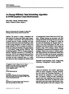
∀t, s,( precede(s,t) ∧ t < s + d(s)) ⇒ t:= s + d(s) Three other symmetrical rules apply to upper bounds. The second set of rules, edge finding, determines if a task can be the first or the last in a given task interval. If t is a task belonging to an interval s, we look at s − t − d(s) . If it is strictly negative, we know that t cannot be the first, therefore t should start after the minimum of (ti + d(ti)) for ti in s other than t (cf. Figure 2). Thus the rule that we apply is the following : ∀t, s,(t ∈s ∧ s − t − d(s) < 0) ⇒ t ≥ min{ti + d(ti ),ti ∈s − {t}}

Here also, a symmetrical rule applies to see if a task can or cannot be the last member of a given interval. Finding the first and last members of task intervals is known as “edge finding” [CC88] [AC91] and is a proven way to improve the search. We will complete these two rules in Section 4.1 with a search strategy that also focuses on edge finding. s-t t

s = t1

[

[

(too small)

] d(s)

]

s = t2

Figure 2: Edge Finding

The previous rule has one drawback, however, because it requires the computation of

min{ti + d(ti ),ti ∈s − {t}}, which is expensive. If we implement this rule with a rule-based language, this rule is likely to be evaluated for many tasks for which it will not increase t. Since using a rule-based implementation has many other advantages (readability, maintainability and flexibility), we improve the rule by using t1 + d(t1 ) (the lower bound of the interval s) as an oracle for min{ti + d(ti ),ti ∈s − {t}}. The rule now becomes : ∀t, s = [t1 ,t2 ],(t ∈s ∧ s − t − d(s) < 0 ∧ t ≤ t1 + d(t1 )) ⇒ t ≥ min{ti + d(ti ),ti ∈s − {t}} The last set of rules, exclusion, tries to order tasks and intervals. More precisely, we check to see if a task can be performed before an interval to which it does not belong (but which uses the same resource). This is done by computing s − t − d(s) − d(t) (same as previously but t no longer belongs to s). If the result is negative, then t cannot be executed before s. We then compute 3The

precede relation with three arguments is used for precedence constraints with delays (e.g. in the bridge problem). precede(t1, t2, d) means that t2 must wait d unit of time after the start of t1 to start.

packed?(s,t) := (d(t) > (s − s − d(s))) If this value is true (cf. Figure 3), then it is not possible to insert t inside s, and thus t must be after s. Otherwise, t must be after the first member of s. Therefore, we use the following rule (and its symmetrical counterpart): ∀t, s = [t1 ,t2 ],t ∉s ∧ s − t − d(s) − d(t) < 0 ⇒

if packed?(s,t) then t ≥ s + d(s) ∧ ∀ti ∈s,ti ≤ t − d(t) else

t ≥ min{ti + d(ti ),ti ∈s}

d(t)

s = t1

[

t

[ ∆

d(s)

]

]t

packed(s,t) = (d(t) > ∆ )

s = t2

Figure 3: Exclusion

Note that we can also avoid computing min(ti + d(ti), ti ∈ s) when t ≥ t1 + d(t1). We have implemented these reduction rules with production rules in LAURE, following previous examples described in [CK92] and [CGL93].

3.3 Interval Maintenance Taking task intervals into account is a powerful technique that allows focusing very quickly on bottlenecks. However, the real issue is the incremental maintenance of intervals. Resources are interdependent because of precedence relationship (As displayed in Figure 4, where the arrows symbolize the precedence constraints). While we are scheduling one resource, the changes of the domains of the tasks are propagated to other resources. We need to be able to compute the changes on intervals very quickly (new active intervals, intervals that are no longer active and changes to the sets associated with the intervals). More precisely, there are two types of events that we need to propagate: the increase of t and the decrease of t . resource 1

resource 2

resource 3 Figure 4: Resource Interdependence

The correct algorithm for updating t can be derived from the definition of the set extension of a task interval: set([t1, t2]) = {t,t1 ≤ t ∧ t ≤ t2 } From this definition, we see that, when increasing the values of t from n to m, • we must deactivate intervals [t,t2] if the new value m is bigger than t2 , • we must remove tasks t’ from active intervals [t,t2] when t’ is less than m,

• we must create new active intervals [t1, t] if m is bigger than t1 and n was not, • we must add t to active intervals [t1, t2] if m is bigger than t1 and n was not and if t is less than t2 . The interesting issue is the order in which we need to perform these operations, and when we are in a state good enough to propagate the changes and trigger the rules. It turns out that negative changes (removing tasks from set extension) do not need to be propagated, because all the rules we use always apply to subsets of intervals (i.e., if a rule can be applied to an interval, it could also be applied to any subset and would not yield more changes). Thus we perform the two “negative” actions first. Then we need to augment the other intervals, which requires triggering rules (as the size or the set extension of intervals changes). This requires that we have set t to its new value m (but not propagated this change yet because the intervals are not set up properly yet). We can legally propagate rules at that point because we know that all intervals have a set extension that can only be smaller than what it should be. Therefore, because of the sets of rules that we are using (monotonic with respect to set containance), we know that any conclusion we might draw will still be valid. The last action is then to propagate the change to t and to update static sets (which we could also do with a propagation rule). To avoid duplicate work, we also need to check that t was not subsequently changed to a higher value by the propagation of a rule. Therefore, we are using two invariants H0 and H1 (cf. the following algorithm) to make sure that we stop all propagation work if m is no longer the new value for t . The algorithm that we use to increase t from n to the new value m is therefore as follows. increase(t,n,m) for i = [t,t2] in [t,_],

;; m > n

if ( n ≤ t2 < m ) ∧ (t2 ≠ t) set(i) := ∅

;; i is no longer active

for t’ in set(i), if ( n ≤ t' < m ) ∧ ( t' < t2 ) do set(i) := set(i) - {t’} d(i) := d(i) - d(t’)

end ;; H0 ⇔ (t = m)

t=m for all t1 ≠ t such that r(t) = r(t1),

;; H1 ⇔ (t1 ≤ m)

if ( n < t1 ≤ m ) for i’ = [t1, t2] in [t1, _], if ( t ≤ t2 ) ∧ H0 ∧ H1

do

set(i’) := set(i’) + {t’}| d(i’) := d(i’) + d(t’) end

for i = [t1, t] in [_,t], if ( t1 ≤ m ) ∧ ( t1 ≤ t ) ∧ H0 if H0 do

do set(i) := {...}, d(i) := ... end

propagate( t = m) for all static sets s that contain t, if (s = n) s := min(...)

The algorithm for decreasing t is exactly symmetrical. We have tried two different variations of this algorithm. First, as mentioned earlier, we tried to restrict ourselves to “critical intervals”, using a total ordering on tasks to eliminate task intervals that represented the same time interval (and thus the same set). It turns out that the additional complexity does not pay off. Moreover, the algorithm is so complex that it becomes very hard to prove. The other idea that we tried is to only maintain the extension of task intervals (represented by a bit vector) and use a function to compute the duration (using a pre-computed duration matrix of size 2n and the bit vector). It turns out that the duration is used very heavily during the computation and that cashing its value improves performance substantially.

4. Application to Some Scheduling Problems 4.1 Search Strategy As we mentioned previously, one of the best branching schemes for the job-shop is to order pairs of tasks that share the same resource [AC91]. The search algorithm, therefore, proceeds as follows. It picks a pair of tasks {t1 , t2 } and a preferred ordering t1 p t2 . The algorithm then explores sequentially the two branches ( t1 p t2 and t2 p t1 ) recursively. This is what most CLP solvers do for scheduling (with simple strategies to pick the pair), and it is very easy to perform with such a language (since backtracking is implicit). To complete the description of our search algorithm, we simply need to describe how we pick the ordered pair (t1,t2). Note that this algorithm produces only a feasible schedule. To get the optimal schedule we must iterate the algorithm many times with decreasing lower bounds. There are, however, better alternatives as we shall discuss later (Section 4.3). The choice of the task pairs is directly inspired from the edge-finding method[AC91], which is itself inspired from the work of Carlier & Pinson [CP89]. The idea is to pick the set of unscheduled tasks for a given resource, and pick a pair of tasks that could be both first (resp. last) in this set. The choice between first and last is based on cardinality. Our adaptation of this idea is to focus on the most constrained subset of tasks for the resource instead of the set of tasks that are currently unscheduled. This allows faster focusing on bottlenecks and takes advantage of the task intervals that we are carefully maintaining. We select, therefore, the task interval i with the smallest slack ∆(i). We compute the set of tasks {t1,..,tp} that could be the first tasks of i and the set of tasks {t’1, ...,t’q} that could be last. We pick {t1,..,tp} if p ≤ q and {t’1, ...,t’q} otherwise. Let's assume from now on that we have picked {t1,..,tp}. Among this set, we need to pick two tasks ta and tb such that ( t a p t b ) and ( t b p t a ) will have the maximal impact (we try to reduce the entropy of the scheduling system, in a manner similar to what is described in [CGL93]). We use the immediate consequence of the ordering ( t a p t b ): t a p t b ⇒ t b := max(t b ,t a + d(t a )) ∧ t a := min(t a ,tb − d(t b )) We decided to pick ta as the lower bound of the interval i. Therefore, if t b < ta, the slack ∆(i) will be reduced by δ = min{t,t ∈i − {t a }} − t a . Our goal is clearly to reduce ∆(i), ∆(ta) and ∆(tb) as much as possible. Thus, we need to give a value to the change ∆ := ∆ − δ, so that we minimize ∆ − δ (the resulting slack) and maximize δ (the change). We have used the following function (where UB is the upper bound for the scheduling problem). f(∆, δ) = if (δ = 0) UB else if (∆ < δ) 0 else (∆ − δ)2 / ∆ Notice that our goal is to obtain a value of f that is as small as possible. Therefore, to evaluate the impact of the decision ( t a p t b ), we compute

δ(ta) = max(t a ,tb − d(tb )) − t a , δ(tb) = tb − min(tb ,t a + d(t a )), and use the value f( t a p t b ) = min(f(∆(ta),δ(ta)), f(∆(tb),δ(tb)). The value associated with the pair (ta, tb) is value(ta , tb) = max(f( t a p t b ), min(f(∆ (i),δ (i)), f( t b p t a )). Notice that we take the change to ∆(i) into account in the case where we try ( tb p t a ). We can now summarize how to select a pair of tasks for a given resource r.

find_pair(r) find i = [t1, t2] in intervals(r) such that ∆(i) is minimal, let S1 = {t | r(t) = r ∧ t ≠ t1 ∧ not(order(t1,t)) ∧ t ≤ t1 + ∆(i) }

;; could be first

S2 = {t | r(t) = r ∧ t ≠ t2 ∧ not(order(t,t2)) ∧ t ≥ t2 − ∆(i)} if |S1| ≤ |S2|

;; could be last

do

δ(i) := Min(t, t∈ i - {t1}) - t1 find t in S1 such that value(t1, t) is minimal return (t1,t) if f(t1 < t) ≤ f(t < t1) and (t,t1) otherwise end

else do

δ(i) := t2 − max{t,t ∈i − {t2 }} find t in S1 such that f(t, t2) is minimal return (t,t2) if f(t < t2) ≤ f(t2 < t) and (t2,t) otherwise end

We use the same high-level strategy as in [AC91]: we choose the most difficult resource as the one with the task interval with the smallest slack. We first schedule this resource totally (i.e., we apply find_pair only to this resource). Then we apply find_pair to all other resources - we minimize break ties ∆(i) with min(|S1|,|S2|).

4.2 Bridge Scheduling As we previously mentioned, the bridge scheduling, which used to be the benchmark of choice for CLP, is nowadays solved easily by most solvers. Typical run-times (CHIP[AB91], PECOS, LAURE) are in the 100 ms range for finding the optimal solution (104 days) and in the 1s for finding the proof of optimality. This proof of optimality is still the longest step, because it requires a number of backtracks (500 to 2000 depending on the search strategy). The first interesting result that we obtain with the previously described algorithm is that the proof of optimality is found with no backtrack (and no search). That means that by simply looking at the right task intervals and by applying the reduction rules that we gave, we can show that there is no solution in 103 or fewer days. A summary of the proof is given in Figure 5. Even for someone who is not familiar with the actual problem, this shows the few steps that allow us to show the optimality on a blackboard without a computer. A consequence is that we are able to solve the problem faster than with previous approaches (cf Figure 6). By “pure CLP” we mean programs that just contain the scheduling constraints. The improved performance is a minor side effect compared to the fact that the whole resolution is done without backtracking. The absence of backtracking is a sign that the algorithm is more powerful and thus will perform better on larger problems. To a certain extent, the results on 10 x 10 job-shop scheduling problems confirm this expectation, but it would be more interesting to use a larger “complex scheduling problem”, with complex precedence constraints. In fact, the bridge scheduling can no longer be considered a benchmark for our algorithm, since it does not really make use of the search strategy. It must also be noticed that the search strategy that we have presented here is designed to optimize the proof of optimality (by minimizing entropy). Other strategies actually work better to simply produce a good solution. We will come back to this issue in the next section, but it is clear that better strategies exist to find the optimal solution (in 104 days) than our method, which is probably too complex here. On the other hand, this complexity provides a robustness (constant performance when the parameters of the problems are changed randomly) that we did not experience with the “pure” CLP solutions. Using a simple heuristic as a starting point, we have been able to reduce the time to obtain the optimal solution to 50ms.

After propagating basic precedence constraints, we have the following domains:

t

t

t^

M1 M2 M3 M4 M5 M6

16 12 26 19 12 18

79 79 79 79 79 79

M5 12

• by looking at [M2, M6] we can tell that M6 is last. • by looking at [Ti, T5] we can tell that all Ti are before T5 • by looking at [T4,T5] we can tell that T4 is first • precedence: [M4, M5] is over by day 33 • by looking at [M4, M5] we can tell that M5 is first

M4 20

M6 61

28

T5 81

32 T4 44

V2

We now have the following domains:

t M1 M2 M3 T1 T2 T3

t 28 28 28 52 44 44

t^ 61 61 61 78 81 81

{M1, M2}

M4

M5 12

• by looking at [T2, T3] we can tell that T1 is not last, so T1 starts in [4,57] • precedence: M1 and M2 are over by day 57 • by looking at [M1,M3] we can tell that M3 is last • precedence: M3 starts after 52 so T3 and T2 start after 60 • {T1,T2,T3} lasts 36 days, cannot fit in [52, 81] => contradiction !

20

28

M6 52

T4 32

T1

61

44

T5 81 V1

V2

Figure 5: Proof of optimality for the bridge

CHIP ([AB91]) LAURE([Ca91]) LAURE pure CLP pure CLP task intervals find optimal solution

160ms

400ms

400ms

proof of optimality

3300ms

1500ms

50ms

total time

3.4 s

1.9s

0.45s

Figure 6: Preliminary results (SPARC-1)

4.3 The MT10 Problem MT10 is a 10 × 10 job-shop scheduling problem that is described in [MT63]. As noticed in [AC91], it is not a very hard 10 × 10 problem, but it has resisted many efforts for a long time and thus has become an interesting benchmark. Using cumulative constraints [AB92], a CHIP program was able to find the optimal solution, after quite a long computation time. Similarly, MT10 was solved in 90 hours with the cc(fd) language [VHSD93], using constructive disjunctions. To our knowledge, no CLP approaches have yet found the proof of optimality in a reasonable time. Therefore, it is a good test for the method based on task intervals. Our first experiment was to look for lower bounds. We use two techniques that we compared with the methods that are currently used in OR approaches [AC91]. First we determined what maximum lower bound value would cause a contradiction when we apply

our reduction rules. This is the method that gave us a 104 lower bound for the bridge problem, so it had already shown to be powerful. For MT10, we obtained 858, which is much better than the lower bounds obtained with other methods (cf. Figure 7). We have also used a common technique, which is to compute the minimal schedule of one machine, but we left the propagation rules active. That is to say that we schedule only one machine, but decisions made on this machine are propagated to the other tasks, which can raise a contradiction. This gives us another lower bound, which is more expensive to obtain (but still less than complex Cuts methods [AC91]). For MT10, we obtained the surprisingly high value of 912. Cuts 1

Cuts 3

Task Intervals

T. Int. 1-Mach

Preempt

1-Mach

value

808

808

823

827

858

912

time

0.1

0.1

5.2

7000

5

200

Figure 7: Lower Bounds for MT10 (from AC91)

These results show the power of task intervals and their reduction rules as a cutting mechanism. We also found similar good results to obtain the proof of optimality (Figure 8). We obtained the proof of optimality in 730 s on a SPARC-1, which is only 2.3 times slower than the special-purpose algorithm of [AC91]. In addition, we explored only 6700 nodes, which is much smaller than the 16000 nodes used by [AC91]. The consequence of these differences will be developed in the next section. To find the optimal solution, we tried several approaches. It must first be noticed that if we use 930 as an upper bound, we find the solution very quickly (40 s). Starting with a high upper bound and reducing gradually produces the optimal solution in 540 s, where most of the time is lost lowering the upper bound to a nontrivial value. Therefore, this solution would need to be coupled with a heuristic, as in [AC91], to give better performance. Starting with the simplest heuristics proposed in [AC91], we can start the search at the value 952 and find the optimal solution in 300 s. We also tried to reduce the upper bound dynamically (instead of re-starting the search after each solution). The results were very similar, in the sense that we got very good results if we had a good starting upper bound (e.g., 955), but that a lot of time was wasted when we started with a very high value (e.g., 1200). We tried to implement the shuffle procedure of [AC91] to improve the convergence, but we obtained very unstable results. Depending on the initial parameters, we would converge very quickly toward the optimal solution or quite slowly towards a suboptimal solution (935). LAURE Task Intervals time nodes MT10 - optimal solution MT10 - proof of optimality LA19 - proof of optimality

540 730 610

6728 6458

ORB2 - proof of optimality

1200

16400

[AC91] time 60 310

nodes

1300

16000 93000

2300

153000

Figure 8: Computational Results for three 10 × 10 Problems (SPARC-1)

These results are preliminary, and further work is needed. We have already confirmed some of our intuition about the low number of backtracks (number of nodes explored) by running the same program on other 10 × 10 problems that were found to be more difficult in [AC91]. LA19 is a problem from [La84] and ORB2 on the problems described in [AC91]. In both cases, we obtained better results than those published in [AC91], using a surprisingly small number of nodes to establish the proof of optimality. The algorithm presented here was designed to build short proofs of optimality, and this shows in the computational results. On the other hand, we spent little time designing good strategies to obtain the optimal

solution quickly. We now plan to turn to this important aspect and see how the search strategy could be modified. In addition, we believe that entropy should play a larger role in the selection of branching pairs for larger problems.

5. Application to the Design of CLP Languages 5.1 Comparison with Non-CLP Approaches It is interesting to compare this approach with the OR approach as related in [AC91] (and also [CC88] and [CP89]) from two different standpoints. On the one hand, we can compare the algorithms, trying to factor out the implementation differences. On the other hand, we can compare the implementation techniques, trying to factor out the differences between the algorithms. As far as algorithms are concerned, different approaches have been used. For instance, the problem can be seen as a linear programming instance and one can use a linear programmation package optimized with plane cuts to solve it (the cuts proposed in [DW90], [Ba69] are summarized in [AC91]). It can also be seen as a graph with symetric arrows that one wants to orient in order to minimize the length of the longest chain. Traditionnal graph techniques include division into smaller problems [Po 88], the use of Petri nets and branch and bound with explicit backtracking (for a complete survey, see [CC88]). More original methods have been proposed, such as [VLAL92] which is derived from statistical physics. The algorithm that we use is actually similar to the one proposed by [CP89] and refined by [AC91]. The cutting equations used in [AC91] are all subsumed by the the propagation on task intervals caused by our rules (ordering, edge finding and exclusion) and by the basic equation (1). The consistent use of reduction rules for all task intervals and not simply for selected ones as in [AC91] explains the lower number of nodes explored by our algorithm. The search strategy is very similar; the two differences are that we focus on the most constrained task interval instead of the wider intervals of unscheduled tasks (as in [AC91]) and we use a different cost function to pick the branching pairs of tasks. Our new heuristic function, based on entropy, seems to give better result that the one used in [AC91] (originally proposed in [ABZ83]). The difference between the performance figures for MT10 are not significant from the algorithm point of view. The code used by [AC91] is hand-optimized C code that took a long time to write. A ratio of 2.3 with the C code generated by the LAURE compiler is a good result and we believe that if our algorithm was implemented directly in C, its performances would improve by such a factor. The real difference between the two algorithms is the lower number of backtracks of our approach, which pays off very strongly with the more complex 10 × 10 problems and is likely to have even more influence for larger problems. For instance, we have been able to improve the lower bound of of the 15 × 10 problem LA21 [La84] from 1039 [AC91] to 1041, which is, to our knowledge, the best value known so far for this open problem. From an implentation point of view, the advantages of our CLP approach are obvious. First, our program can handle job shop problems as well as problems with more complex dependencies (e.g. the bridge scheduling). If we start with the jobshop program, we can add static sets with a few as 30 lines of LAURE code that are totally independent from the earlier code. This is much harder for hand-optimized algorithms written in C. The flexibility comes from the use of logical rules, which create a nonexplicit binding between components of the software and allow us to add new rules representing new constraints or new heuristics without changing a line of the original program. The second advantage of the CLP approach is its simplicity. Through the use of a highlevel programming language and a limited number of redundant constraints, we have kept the size of the LAURE program under 400 lines (without counting the data definition part). This is much longer than the 40 lines of the original CLP program from which we started, but much shorter than the 2000 lines of C code of the similar program from [AC91]. In addition, the use of high-level programming paradigms (such as sets, objects or rules) makes the code

much easier to read and maintain. Another measure is that the program was written in a few days, then it was tuned and optimized within 2 weeks.

5.2 Comparison with Similar CLP Approaches It is easy to compare this new LAURE program with the scheduling program that we used before. As stated previously, the program has lost its original simplicity since we went from 40 to 400 lines of code, but it has also gone from a naive and declarative style of programming to a more expert style. However, we have obtained an improvement in performance and robustness that make the new program able to compete with the best OR algorithm, which was definitely not the case for the simpler program. For instance, the MT10 problem cannot be solved with the simple, generic approach of our 40-line program. These remarks obviously apply to the similar programs that one could write with CHIP or PECOS, since we had previously shown LAURE to be among the best available finite-domain constraint solvers. It is interesting to notice that the new approach could also have been implemented with PECOS, which is a lower-level language than LAURE (i.e., it does not support logical rules), although with a bigger programming effort. On the other hand, CHIP is somehow a higher-level (of abstraction) language than LAURE, since it does not provide the same control and access to the data structures of the constraint solver. As a consequence, writing an efficient program that uses task intervals in CHIP is a much harder task. CHIP has followed a different direction and included an additional type of cumulative constraint [AB92]4. These constraints encapsulate some of the OR techniques that we have mentioned previously, although the exact behavior of the cumulative constraint is proprietary information. These techniques allowed CHIP to be the first CLP language to find the optimal solution of the MT10 problem, but they fell short of providing performances that are competitive with OR dedicated algorithms. For instance, the proof of optimality for MT10 is still out of reach within reasonable computation time. Cumulative constraints are more general than a simple one-machine scheduler, but these results show that a user of CHIP with cumulative constraint would get much better performance using task intervals. This leads to the most interesting question: Should a technology such as task intervals be packaged into a closed component, such as a cumulative constraint, or should the user understand how it works and have access to its implementation ? If we go back to the CHIP example, we believe that the designers of the compiler can easily pick the ideas presented in this paper and make their system as efficient as the LAURE program presented here (and maybe more efficient, since they are implementing their code in a black-box manner). However, we do not believe that this solution would match the needs of the users. Our experience with large, real-life problems is that no generic search techniques (even as successful as task intervals) are powerful enough to solve them. It takes the domain-dependent expertise of the user to make the right combination of such techniques to solve the problem. This is why we were looking for a simple and powerful technique that could be explained to anyone, as opposed to a clever algorithm that we would implement into the LAURE system. It would be very easy to package resources with task intervals as a first-class LAURE constraint, which would allow us to claim much shorter programs with similar good performance. Our claim is that packaging it as a set of rules with associated methods [Ca91] makes it easier for the user to pick the components that are necessary for his problem.

5.3 A CLP User’s Wish List The previous postulate in favor of a “white-box” implementation of techniques such as task intervals has a profound impact on what a CLP language should offer. We have already addressed some of the issues in earlier papers [Ca91], but we believe that the previous 4

There has been a lot of work about general search principles and handling of disjunctive constraints that is relevant to job shop scheduling (e.g. [dBB93], [VHSD93]), some of which was actually included into the generic LAURE solver. However, to our knowledge, using only generic techniques has not lead to performances comparable to OR algorithms on problems such as MT10.

findings on job-shop scheduling give more strength to these ideas. Here is a list of the three major features that we are expecting from a CLP language that should be self-evident from the algorithm proposed in Section 3. • Backtracking over user-defined structure. All CLP languages provide automatic backtracking over the logical variables that define the problem. However, in most problems, additional data structures need to be maintained. In this example, we used task intervals. In a staff scheduling problem [CGL93], we used a min/max global matrix. Using additional data structures is enormously simplified if changes can be backtracked automatically. The only task left to the user is to describe how choices made by the constraint solver will impact the data structure. • Control over search strategy. It is also clear that generic search strategies, such as the first-fail principle, are not a panacea. In many of the complex problems that we have solved, what is needed is a dynamic generation of branching goals. This means that we need more than being able to redefine the ordering of goals. We really need complete control over the search strategy. • Semi-explicit propagation. Quite often, changes to the external data structure must be made when a (complex) logical condition is satisfied. The reduction rules that we gave in Section 3 are good examples. Being able to write this declaratively with a logical rule makes the programming task much easier. The alternative would be to examine the logical condition and determine all the cases when the conclusion must be evaluated, which is a tedious and error-prone process. This last feature is less critical, since we can always return to explicit propagation in a procedural way. However, rule-based propagation helps retain many of the desirable features of “naive” CL programming, such as readability and flexibility.

6. Conclusion This new technique for job scheduling focusing on intervals of tasks gives a very good representation of the problem, and its incremental maintenance makes it efficient. The logical rules, although quite simple, subsume most cuts used by traditional OR techniques ([Ba69], [CP89], [DW90], [AC91]). The search heuristic is efficient because it focuses on bottlenecks. Using logical rules brings much flexibility: the authors were surprised by how fast they could adapt the program from the bridge problem to n × m scheduling problems. More results are expected soon. From the results on the bridge problem and on MT10, we draw two conclusions: • First, CLP is a technology of choice for these hard combinatorial problems because it can combine efficiency and flexibility. As a matter of fact, we now project incorporating this algorithm in other programs that involve, among other things, job scheduling. • Second, our methodology (refining step by step a naive logical description of the problem) has brought, up to now, tremendous results. Thus it seems very important that constraint logic language designers give programmers the necessary transparency to allow such programming.

Acknowledgments This paper and the work on job-shop scheduling has been strongly influenced by conversations with Bill Cook, Francois Fages, Jean-Francois Puget and Pascal Van Hentenryck.

References [ABZ83]

J.Adams, E. Balas & D. Zawak. The Shifting Bottleneck Procedure for Job Shop Scheduling. Management Science 34, p391-401. 1983 [AB91] A. Aggoun, N. Beldiceanu. Overview of the CHIP Compiler. Proc. of the 8th ICLP, Paris, 1991. [AB 92] A. Aggoun, N. Beldiceanu. Extending CHIP in order to Solve Complex Scheduling and Placement Problems. Proc. of JFPL'92 (Journées Francophones sur la Programmation Logique), Lille (France), May 1992. [AC91] D. Applegate & B. Cook. A Computational Study of the Job Shop Scheduling Problem. Operations Research Society of America vol 3, no 2, 1991 [Ba 69] E. Balas. Machine Sequencing via Disjunctive Programming: an Implicit Enumeration Algorithm. Operations Research 17, p 941-957. 1969 [Ca91] Y. Caseau: A Deductive Object-Oriented Language. Annals of Mathematics and Artificial Intelligence, Special Issue on Deductive Databases, March 1991. [CC88] J. Carlier & P. Chretienne. Problemes d'ordonnancement. col. ERI, Masson, Paris 1988 [CGL93] Y. Caseau, P.-Y. Guillo, E. Levenez. A Deductive and Object-Oriented Approach to a Complex Scheduling Problem. Proc. of DOOD'93, Phoenix, December 1993. [CK92] Y. Caseau, P. Koppstein. A Cooperative-Architecture Expert System for Solving Large Time/Travel Assignment Problems. International Conference on Databases and Expert Systems Applications, Valencia, Spain, September 1992. [CP89] J. Carlier & E. Pinson. An Algorithm for Solving the Job Shop Problem. Management science, vol 35, no 2, february 1989 [dBB93] B. de Backer, H. Beringer. A CLP language handling disjunctions of linear constraints. Proc. of 10th ICLP, The MIT Press,1993. [DW90] M. Dyer & L.A. Wolsey. Formulating the Single Machine Sequencing Problem with Release Dates as a Mixed Integer Program. Discrete Applied Mathematics 26, p255-270. 1990 [La84] S. Lawrence. Resource Constrained Project Scheduling: an Experimental Investigation of Heuristic Scheduling Techniques. GSIA, Carnegie Mellon University 1984 [MT63] J.F. Muth & G.L. Thompson Industrial scheduling. Prentice Hall, Englewood Cliffs, NJ, 1963 [PA91] J.F. Puget, P. Albert. PECOS: programmation par contraintes orientée objets. Génie Logiciel et Systèmes Experts, vol. 23, 1991. [Po88] M.C. Portmann. Methodes de Decomposition Spatiale et Temporelles en Ordonacement de la Production. RAIRO vol 22, no 5, 1988 [VLA92] P. Van Laarhoven, E.Aarts & J.K. Lenstra. Job Shop by Simmulated Annealing. Operations Research vol 40, no 1, 1992 [VH89] P. Van Hentenryck: Constraint Satisfaction in Logic Programming. The MIT press, Cambridge, 1989. [VHSD93] P. Van Hentenryck, V. Saraswat, Y. Deville. The Design, Implementation, and Applications of the Constraint Language cc(FD). Brown University Technical Report, 1993.