Hindawi Publishing Corporation Shock and Vibration Volume 2016, Article ID 4593749, 13 pages http://dx.doi.org/10.1155/2016/4593749
Research Article Improved Element Erosion Function for Concrete-Like Materials with the SPH Method Jilí Kala and Martin Hušek Faculty of Civil Engineering, Brno University of Technology, Veveˇr´ı 331/95, 602 00 Brno, Czech Republic Correspondence should be addressed to Jiˇr´ı Kala;
[email protected] Received 21 December 2015; Revised 27 February 2016; Accepted 7 March 2016 Academic Editor: Matteo Aureli Copyright © 2016 J. Kala and M. Huˇsek. This is an open access article distributed under the Creative Commons Attribution License, which permits unrestricted use, distribution, and reproduction in any medium, provided the original work is properly cited. The subject of the paper is a description of a simple test from the field of terminal ballistics and the handling of issues arising during its simulation using the numerical techniques of the finite element method. With regard to the possible excessive reshaping of the finite element mesh there is a danger that problems will arise such as the locking of elements or the appearance of negative volumes. It is often necessary to introduce numerical extensions so that the simulations can be carried out at all. When examining local damage to structures, such as the penetration of the outer shell or its perforation, it is almost essential to introduce the numerical erosion of elements into the simulations. However, when using numerical erosion, the dissipation of matter and energy from the computational model occurs in the mathematical background to the calculation. It is a phenomenon which can reveal itself in the final result when a discrepancy appears between the simulations and the experiments. This issue can be solved by transforming the eroded elements into smoothed particle hydrodynamics particles. These newly created particles can then assume the characteristics of the original elements and preserve the matter and energy of the numerical model.
1. Introduction When a projectile flying at high speed collides with a concrete surface, its kinetic energy drops to zero but the internal energy of the system increases sharply. The response of the concrete surface to this type of load often takes the form of irreversible (plastic) deformations. If the kinetic energy of the projectile is sufficiently great and the body of the projectile is sufficiently stiff, penetration of the concrete surface occurs. This type of failure is also accompanied by the chipping off of the concrete and the development of dynamically propagating cracks. The successful execution of numerical simulations of this phenomenon is very difficult, however, particularly when the finite element method (FEM) is used. In order for the results of FEM simulations to correspond with the results of experiments, it is necessary to combine suitable material models with numerical model failure techniques, but it is also essential to avoid numerical problems which often negatively affect the results of the simulations. Today, thanks to constantly ongoing research into concrete structures, extensive concrete material model databases are available and often implemented in commercial programs
such as LS-DYNA [1]. The options and conditions for the use of a given selected material model are, however, often open to debate [2]. On top of that, before the execution of the simulation an assumption often has to be made regarding the type of failure that will be decisive so it is possible to select a material model at all [3]. The response of the concrete also depends on the character of the load [4–7], which makes the choice even more complicated. Generally, in the case of high-speed loading it is necessary to use a material model which takes strain rate into consideration [8–10]. In such cases, equations of state (EOS) are often used to enable the successful description of the material model due to the fact that bodies behave in a similar manner to fluids when under high-speed loading. As far as the software is concerned, an algorithm has to be accessible which will interpret such information appropriately for the computational process. This is enabled, for example, by the previously mentioned LS-DYNA program [1] and also AUTODYN [11]. The HJC model [12, 13] (named after its authors Holmquist, Johnson, and Cook) can then be a suitable material model, as it has the above-mentioned properties; it considers the strain rate and utilizes EOS for description.
2 However, simulations also need to include a numerical technique which will enable the simulation of continuum failure; in the case of the FEM method, this takes the form of the failure of the finite element mesh. If this technique was not used, the simulation of, for example, the chipping off of material or the perforation of the loaded structure would not be possible. Additionally, numerical problems (the locking of elements, negative volumes, etc.) could arise due to the influence of excessive deformations (distortion of elements). The numerical erosion of finite elements can be such a technique. Even though numerical erosion is primarily used to filter out problem elements from the calculation, it can also be suitably used to aid in the simulation of cracks, penetration or perforation, and also the fragmentation of matter. The technique of combining the FEM and element erosion is often used in high-speed simulations, particularly in the simulation of penetration and perforation [14–19]. However, the criterion of element erosion is not unambiguous [20] and can affect the results of the simulation [11]. For example, the damage parameter is selected as an erosion parameter in [14], while in [15] it is maximum tensile stress, in [16, 18] it is geometric strain, in [17] it is fracture strain, and in [19] the erosion parameter is a combination of the damage parameter value and the maximum principal strain. Despite the use of advanced numerical techniques, the results of simulations are still being compared, most frequently with the values from analytical relationships obtained from an extensive amount of experiments [21, 22]. In the case of specific simulations, results are compared directly with experiments such as [23]. Unfortunately, as a result of the heterogeneity of the structure of concrete, agreement between simulations [24] and experiments cannot be guaranteed despite the use of complex modelling techniques. The dissipation of matter from calculations as a result of the deletion of elements can be a significant problem in cases where the numerical erosion technique is used. In the majority of cases, this problem is omitted and left unsolved [14–19]. So, why use the FEM method for high-speed load simulations when so many problems and complications arise during calculations? With regard to the existence of meshfree methods such as smoothed particle hydrodynamics (SPH), it is possible to realize high-speed load simulations without needing to include numerical erosion or deal with problems concerning the dissipation of matter [25, 26]. There are several reasons for preferring the FEM method, the main one being the low computational requirements compared with the aforementioned SPH method. Even though the SPH method can be a good choice for high-speed simulations of dynamic events, even in this case many numerical difficulties arise (tensile instability, zero-energy modes, etc.) which need to be resolved; see also [27–29]. However, if the strong points of the FEM and SPH methods were combined, a very useful apparatus for dealing with high-speed simulations could be created. With regard to the facts mentioned above, the aim of the paper is to propose a procedure for the execution of simulations of the high-speed loading of concrete by steel projectiles. This approach will combine the FEM method with the numerical erosion of elements, and its primary focus
Shock and Vibration will be on solving the problem with matter dissipation. This dissipation can be prevented via the transformation of eroded elements into SPH particles. In addition, current procedures for dealing with such simulations which do not introduce either the erosion of elements or the transformation of eroded matter will be compared. The concept of combining the FEM and SPH techniques with the inclusion of element erosion aims mainly at the improvement of simulation techniques in cases of high-speed loading in such a way that possible numerical issues are minimized and the results of simulations correspond better to the results of experiments.
2. The Erosion Problem The element erosion function, while not a material property or physics-based phenomenon, provides a useful means of simulating the spalling of concrete and provides a more realistic graphical representation of actual impact events. Erosion is characterized by the physical separation of the eroded solid element from the rest of the mesh [30]. Though element removal (erosion) associated with total element failure has the appearance of physical material erosion, it is, in fact, a numerical technique used to permit the extension of the computation. Without numerical erosion, severely crushed elements in Lagrangian calculations would lead to a very small time step, resulting in the use of many computational cycles with a negligible advance in the simulation time. Moreover, Lagrangian elements which have become very distorted have a tendency to “lock up,” thereby inducing unrealistic distortions in the computational mesh [31]. The erosion function allows the removal of such Lagrangian cells from the calculation if a predefined criterion is reached. When a cell is removed from the calculation process, the mass within the cell can either be discarded or be distributed to the corner nodes of the cell. If the mass is retained, the conservation and spatial continuity of inertia are maintained. However, the compressive strength and internal energy of the material within the cell are lost whether the mass is retained or not. Even though the filtering out of unsuitable (unneeded) elements is more a matter for numerical simulations, it can be connected (to a certain degree) with the physical matter of the material model. 2.1. Residual Compressive Strength with SPH. The moment at which an element of the Lagrangian mesh erodes is in conflict with what happens in real life, however. In reality, the material does not cease to exist but is only crushed and flakes off; see Figure 1. Even though one cannot speak about the strength of the material as such, the particles and wedge-shaped fragments that fly off can create secondary or residual strength. In order to better approximate reality, it is advantageous to maintain the presence of even such particles in the simulation. This can be done via the transformation of eroded elements into SPH particles. Subsequently, these freely moving particles with the characteristics of the original materials will interact with the rest of the computational model and thus better reflect reality.
Shock and Vibration
3
Scabbing Spalling
(a) Penetration and spalling
(b) Scabbing
(c) Perforation
Figure 1: Schematic diagrams showing penetration, scabbing, and perforation of concrete slabs struck by “hard” missiles.
3. The SPH Method Smoothed particle hydrodynamics (SPH) is a mesh-free, Lagrangian particle method, originally developed for modelling fluid flows [32]. In 1982 Zukas first used the SPH method for modelling high-speed impact events [33]. Since high-speed impacts and penetration processes usually involve large deformations, their simulation is generally difficult for traditional grid-based numerical methods such as the FEM. The SPH method is, on the other hand, a particularly suitable candidate for these types of problems. 3.1. Essential Formulation of the SPH Method. The formulation of the SPH method is often divided into two key steps. The first step is the integral representation of field functions and the second is particle approximation. The concept of the integral representation of a function 𝑓(x) used in the SPH method starts from the following identity: 𝑓 (x) = ∫ 𝑓 (x ) 𝛿 (x − x ) 𝑑x , Ω
(1)
where 𝑓 is a function of the three-dimensional position vector x and 𝛿(x − x ) is the Dirac delta function given by {+∞ x = x 𝛿 (x − x ) = { 0 x ≠ x . {
(2)
In (1), Ω is the volume of the integral that contains x. Equation (1) implies that a function can be represented in an integral form. Since the Dirac delta function is used, the integral representation in (1) is exact or rigorous as long as 𝑓(x) is defined and continuous in Ω [32]. If the Delta function 𝛿(x − x ) is replaced by a smoothing function 𝑊(x − x , ℎ), the integral representation of 𝑓(x) is given by 𝑓 (x) ≈ ∫ 𝑓 (x ) 𝑊 (x − x , ℎ) 𝑑x , Ω
(3)
where 𝑊 is the so-called smoothing function and ℎ is the smoothing length defining the influence area of the smoothing function 𝑊. Note that as long as 𝑊 is not the Dirac
Integration domain, Ω Support domain of smoothing function for particle i
Smoothing function, W
i rij
𝜅h
j
Figure 2: Particle approximations using particles within the support domain of the smoothing function 𝑊 for particle 𝑖.
delta function, the integral representation in (3) can only be an approximation [32]. The continuous integral representations concerning the SPH integral approximation in (3) can be converted into discretized forms of summation over all the particles in the support domain shown in Figure 2. The corresponding discretized process of summation over the particles is commonly known as particle approximation. If the infinitesimal volume 𝑑x in (3) at the location of particle 𝑗 is replaced by the finite volume of the particle Δ𝑉𝑗 that is related to the mass of the particles 𝑚𝑗 by 𝑚𝑗 = Δ𝑉𝑗 𝜌𝑗 ,
(4)
where 𝜌𝑗 is the density of particle 𝑗(= 1, 2, . . . , 𝑁) in which 𝑁 is the number of particles within the support domain of particle 𝑗, then the continuous SPH integral representation for 𝑓(x) can be written in the following form of discretized particle approximation [32]: 𝑁
𝑓 (x) ≈ ∑ 𝑗=1
𝑚𝑗 𝜌𝑗
𝑓 (x𝑗 ) 𝑊 (x − x𝑗 , ℎ) .
(5)
Equation (5) states that the value of a function at particle 𝑖 is approximated using the average of those values of the
4
Shock and Vibration
function at all the particles in the support domain of particle 𝑖 weighted by the smoothing function, shown in Figure 2. In Figure 2, 𝜅 is a constant related to the smoothing function for particle 𝑖 and defines the effective (nonzero) area of the smoothing function. This effective area is called the support domain for the smoothing function of particle 𝑖. The adaptability of SPH is achieved by performing particle approximation at each time step based on particles arbitrarily distributed in the current support domain. Because of this adaptive SPH approximation performed at the very early stage of field variable approximation, the formulation of SPH is not affected by the arbitrariness of the particle distribution as it changes with time. It can therefore naturally handle problems involving extremely large deformation [32]. More information about the construction of the smoothing function can be found in [34].
4. The HJC Material Model Under shock wave compression, plastic deformation and crack-induced damage should be taken into account in the modelling of concrete behaviour. A constitutive law combining pressure-dependent plastic hardening, damagesoftening, and the strain rate effect, especially suited for the prediction of concrete response under dynamic loading such as blasts and impacts [35], was developed by Holmquist et al. [12]. In this constitutive law the normalized equivalent stress is defined as 𝜎∗ = [𝐴 (1 − 𝐷) + 𝐵𝑃∗𝑁] [1 + 𝐶 ln (𝜀∗̇ )] ≤ 𝑆max ,
(6)
where 𝜎∗ = 𝜎/𝑓𝑐 and 𝑃∗ = 𝑃/𝑓𝑐 are the normalized equivalent stress and pressure, with 𝜎 and 𝑓𝑐 being the actual equivalent stress and the quasi-static uniaxial compressive strength, respectively. Scalar damage 𝐷 is a value from 0 to 1 that describes the accumulation of damage as a percentage of the full cohesive strength that the material possesses. When 𝐷 = 0, the material is undamaged and exhibits its full strength, but at 𝐷 = 1 the material is fully damaged and retains the least confined shear strength. 𝜀∗̇ = 𝜀/̇ 𝜀0̇ is the dimensionless strain rate, where 𝜀̇ and 𝜀0̇ are the actual and reference strain rates, respectively. The material constants are 𝐴, 𝐵, 𝐶, 𝑁, and 𝑆max , where 𝐴 is the normalized cohesive strength, 𝐵 is the normalized pressure hardening coefficient, 𝐶 is the strain rate coefficient, 𝑁 is the pressure hardening exponent, and 𝑆max is the normalized maximum strength that can be developed. The model accumulates damage from both equivalent plastic strain Δ𝜀𝑝 and plastic volumetric strain Δ𝜇𝑝 . The compression damage is expressed as 𝐷=∑
Δ𝜀𝑝 + Δ𝜇𝑝 𝐷1 (𝑃∗ + 𝑇∗ )𝐷2
,
(7)
where 𝐷1 and 𝐷2 are material constants; 𝑇∗ = 𝑇/𝑓𝑐 is the normalized maximum tensile hydrostatic pressure that the material can withstand; and 𝑇 is the maximum tensile hydrostatic pressure.
The equation of state (EOS linear elastic region, transition region, and compact region) is expressed as follows [12, 13] for loading: 𝑃 𝐾elastic 𝜇 { { { { { { (𝑃 − 𝑃crush ) (𝜇 − 𝜇crush ) = {𝑃crush + lock { (𝜇lock − 𝜇crush ) { { { { 2 3 {𝐾1 𝜇 + 𝐾2 𝜇 + 𝐾3 𝜇
0 ≤ 𝜇 ≤ 𝜇crush 𝜇crush < 𝜇 ≤ 𝜇lock
(8)
𝜇 > 𝜇lock ,
where 𝜇 = 𝜌/𝜌0 − 1 is the standard volumetric strain; 𝐾elastic = 𝑃crush /𝜇crush is the elastic bulk modulus; 𝜌 and 𝜌0 are the current and initial densities, respectively; 𝜇crush and 𝜇lock are the crushing and locking volumetric strains, respectively; 𝑃crush and 𝑃lock are the crushing and locking pressures; and 𝐾1 , 𝐾2 , and 𝐾3 are pressure constants; see Figure 3. The modified volumetric strain 𝜇 is defined as 𝜇=
(𝜇 − 𝜇lock ) . (1 + 𝜇lock )
(9)
The tensile pressure is limited to 𝑇(1 − 𝐷) during numerical calculations. 4.1. Implementation of Erosion. The HJC material model offers the implementation of element erosion on the basis of the size of the damage strength, 𝐷𝑠 . The damage strength, 𝐷𝑠 , is defined in compression when 𝑃∗ > 0 as 𝐷𝑠 = 𝑓𝑐 min [𝑆max ; 𝐴 (1 − 𝐷) + 𝐵𝑃∗𝑁] [1 + 𝐶 ln (𝜀∗̇ )]
(10)
or in tension if 𝑃∗ < 0, as 𝐷𝑠 = 𝑓𝑐 max [0; 𝐴 (1 − 𝐷) − 𝐴 (
(11) 𝑃∗ )] [1 + 𝐶 ln (𝜀∗̇ )] . 𝑇
The element erodes at the moment when its damage strength 𝐷𝑠 falls below 0. From the physical point of view the implementation of such an algorithm is justified [1]. 4.2. Transformation of Eroded Elements. If the abovementioned problem with eroded matter and its dissipation were not solved, in extreme cases results might be gained which appear not to make sense. An example of this can be found in Figure 4, where a concrete specimen impacts a rigid base at high speed. At the moment when the sample comes into contact with the base, it starts to be crushed. The kinetic energy of the specimen transforms into plastic deformations of its body, and the specimen thus starts to slow down. Figure 4 compares the progression of the impact of the specimen when its numerical description does not enable erosion of the elements (on the left) and when it does enable such erosion (in the middle). It is obvious that the results are significantly different in the final stage. The top surface
5
Normalized equivalent stress, 𝜎∗ = 𝜎/fc
Shock and Vibration
Strength D = 0 (undamaged)
Smax
T∗ (1 − D)
D = 1.0 (fractured) .∗
𝜀 > 1.0 𝜀∗ = 1.0 .
A
𝜎∗ = [A(1 − D) + BP∗N ][1 + C ln 𝜀∗ ] .
Normalized pressure, P∗ = P/fc
Damage
Pressure (Δ𝜀p + Δ𝜇p ) f
P = K1 𝜇 + K2 𝜇2 + K3 𝜇3
f
f
𝜀p + 𝜇p
f
Pressure, P
(𝜀 p + 𝜇 p )
f
D=∑
𝜇=
𝜇 − 𝜇lock 1 + 𝜇lock
𝜀min
T∗
f
f
(𝜀p + 𝜇p ) = D1 (P∗ + T∗ )D2
Plock Pcrush
P∗
𝜇crush T(1 − D)
𝜇lock 𝜇 = 𝜌/𝜌0 − 1
Figure 3: Graphical representation of the HJC material model [12].
of the specimen with element erosion almost falls onto the base, while the top part of the specimen without such erosion remains at half its original height. Even though the assumption was introduced that the only elements which will be eliminated from the calculation are those that would be in the stage of full failure from the perspective of the material model and therefore would not influence the further course of the simulation significantly, it is obvious from the results that such a simple implementation of numerical erosion is inadequate, even if it is linked to the material model. The third variant of the sample in Figure 4 (on the right) includes the adaptive transformation of eroded elements into SPH particles. These particles have assumed the material properties of the eroded elements and their weight and speed, but also their stress state and so forth. More information on SPH can be found in [32]. It can be concluded from the results that the described residual strength appears thanks to SPH particles. This strength is represented by the interaction of SPH particles with the rest of the numerical model and simultaneously with one another. The variant of the model with SPH particles then
corresponds well with the original model where erosion was not included. Mass of the specimen through the simulation is shown in Figure 5.
5. Combination of FEM and SPH The motivation for the combination of the FEM and SPH methods is mainly the need to filter out numerical problems in cases involving large deformations (FEM), but it is also due to the need to lower the computational requirements of the simulations (SPH). As was stated in Section 3.1, the SPH method can deal with problems concerning large deformations while avoiding numerical complications thanks to its adaptive nature. However, the issues with computational requirements cannot be solved absolutely conclusively, particularly in the case of the SPH method. It is true for both methods that the computational requirements (time requirements) increase as the number of elements or particles grows. These requirements can be reduced to a certain degree. In the case of the FEM, the quality and computational requirements of the solution are closely connected with the
6
Shock and Vibration No erosion
Erosion
Erosion + SPH
Figure 4: Phases of the impact of a concrete specimen. From the left: model variant with no erosion, with erosion, and with erosion and adaptive transformations into SPH.
Mass of the specimen (%)
120.0 100.0 80.0 60.0 40.0 20.0 0.0 0.0
0.5
1.0
1.5
2.0 2.5 Time (ms)
3.0
3.5
No erosion Erosion Erosion + SPH
Figure 5: Mass of the specimen through the simulation.
4.0
number of integration points in the element. If numerical complications of the hourglass type are solved, reduced element integration can be used, one integration point per element. Moreover, numerical integration takes place most frequently in the reference element, which is an advantage [36]. In the case of the SPH method, the integration points also represent particles (one integration point per particle), while the numerical integration takes place in the form (5). This means that, in the case of both the FEM and the SPH methods, the computational requirements do not necessarily have to increase above all limits as a result of the increasing number of elements or SPH particles. However, there is a problem with the SPH method: it is necessary to search for neighbouring particles within the support domain and perform other associated operations
Shock and Vibration
7
CPU time (s)
10000
8733
8000 6000 4000
3985
3268
2538
2000 0
FEM no erosion
FEM erosion
FEM erosion + SPH
SPH only
Figure 6: Comparison of CPU times needed for simulation computation. Projectile impact speed: 500 ms−1 .
Displacement
Displacement convergence
Mesh/particle distribution density Exact solution FEM/SPH solution
Figure 7: The quality of the solution with increasing spatial discretization density.
in each time step of the explicit algorithm for the solution of a nonstationary task. The size of the support domain can also be different in every step (and actually is in the majority of cases). A small domain size can result in a lowaccuracy solution, while a large support domain can cause the smoothing of local properties [32]. If, however, there was no search for nearby particles in each time step, the adaptability of the SPH method would be lost. This would mean losing the capability to successfully investigate excessive deformations. With a combination of the FEM and SPH method a good balance is attained between computational requirements and the quality of the achieved results. Figure 6 shows a comparison of the calculation lengths required by simulations of the experiment described in Section 6, for a 500 ms−1 projectile impact speed and different numerical model variants. 5.1. Mesh Density and SPH Regularity. In the case of the FEM [37] and SPH [32] methods, the accuracy of the result generally increases with the increasing density of the finite element mesh or SPH particle distribution; see the diagram in Figure 7. In the case of a combination of material damage models and FEM, localized damage can occur if such dependencies are not filtered out [38]. In the majority of cases such damage concentrates in the smallest element, or the element with the lowest stiffness. With increasing FEM mesh density, failure types can occur which do not correspond with reality. This
Figure 8: Inactive SPH particles placed in the centre of gravity of the FEM elements.
issue can be dealt with in several ways. If there are links to the fracture energy of the material in the description of the material model, the dependence between the size of the finite element and the shape of the stress-strain diagram [38] can be used; the stress-strain diagram will be altered for various element sizes. If the material model does not include fracture energy, a solution can be achieved via the connection of a nonlocal model [39]. The nonlocal treatment basically attempts to average out the failure/damage values of neighbouring elements in order to minimize the mesh dependency of the results [40]. This technique was also applied to the HJC material model. The SPH method is also influenced by the density of the particle distribution. However, the regularity of this distribution in the initial stage of the simulation is a greater problem [1]. In the case of a bad distribution, particle clusters can be created. Such locations in the support domain would then contain large quantities of particles. In contrast, very sparsely populated areas can appear. As a result of such clusters, false cracks may occur. They may also have an effect on the behaviour of real cracks, which have the tendency to bypass places where clusters occur. This problem with the SPH method still has not been resolved. Due to this, a regular finite element mesh distribution was maintained in the simulation so that no clusters occur in the SPH particles as they appear. In the simulation of the experiment from Section 6, studies examining the dependence of the result on the density of the finite element mesh or the regularity of such distribution were not carried out. Nevertheless, such studies are planned for future research. The FEM elements in the area around the point of impact were approximately 1/20 of the projectile’s diameter in size. 5.2. From FEM to SPH. An SPH particle is created at the moment when an FEM element erodes. The conditions for element erosion during simulations are shown in (10) and (11). The SPH particles are included in the calculation from the beginning so that their position and other characteristics can be determined as they appear during the simulation. The position most frequently selected for them is in the centre of gravity of the FEM elements. However, the particles are inactive so that there is no increase in computational requirements. Inactive particles are marked grey in Figure 8. After the erosion of FEM elements, there are two ways in which interaction can take place between the SPH particles
8
Shock and Vibration ∼6.350
2.54
Figure 9: Interaction between FEM elements and SPH particles via the penalty-based contact method.
5.385 ± 0.02
35∘ ± 0.5
Figure 11: Shape and dimensions of the projectile (units in mm).
Figure 10: Interaction between FEM elements and SPH particles via a transition layer.
and the undamaged FEM model. The first option is via a contact formulation, most frequently the penalty method. This is drawn schematically in Figure 9. In Figure 9, already active SPH particles are shown in green, while inactive SPH particles are coloured grey. The layer of FEM elements for which the contact algorithm is active is marked in red. The second option is the creation of a transition layer on the interface between the FEM elements and SPH particles. This transition layer then contains FEM elements as well as active SPH particles, which are coupled. This is drawn schematically in Figure 10. Again, active SPH particles are green, inactive SPH particles are grey, and SPH particles that are coupled with FEM elements to create a transition layer are marked blue. Transition layers were used in the simulation of the experiment from Section 6. It is expected that future studies will be conducted where the variable will be the amount of SPH particles placed in the element.
6. The Experiment and Simulation In 2002 Buchar et al. performed an experiment with projectiles; see Figure 11, defined by the NATO STANAG 2920 standard, which they shot at speeds of 300–1400 ms−1 into concrete targets with the dimensions 0.1 × 0.1 × 0.1 m and a strength in compression of 43.1 MPa [41]. The mass of the projectiles was 1.102 g. A good correlation was then found between the performed experiments and the theory applied according to [42]. 6.1. Setting Up the Simulation. The most important simulation settings are described in the tables, where Tables 1 and
2 describe material properties, Table 3 describes the setting of the SPH formulation, and Table 4 describes the setting of the FEM mesh. The simulations were carried out in the LSDYNA program [1], in which robust explicit method solvers are implemented. LS-DYNA also enables the execution of simulations using the FEM as well as SPH methods, or their combination. The chosen size of the coefficient of friction between the concrete block and the projectile was between 0.1 and 0.45. However, studies have shown that the amount of friction does not have a significant influence on penetration depth. This is because a ballistic cavity is created in the surroundings of the projectile as it impacts and subsequently penetrates the concrete slab at high speed. As a result of the creation of this cavity, the influence of side friction between the projectile and the concrete slab is eliminated. However, this can be just a temporary extension, a temporary cavity. In the majority of cases, however, the surrounding area chips off. 6.2. Results of the Simulation. The results of the numerical simulation of the experiment are presented in graphical form in Figure 12. The image shows the stages of penetration of a projectile with an impact speed of 500 ms−1 . Once again, on the left, there is the numerical model without element erosion, in the middle there is the model with erosion, and on the right there is the model which also contained the transformation of eroded elements into SPH particles. The size of the crater in the final stage of penetration (i.e., the quantity of eroded elements) increased exponentially with the growing impact speed of the projectile. This was echoed by the considerably greater depth of penetration for model with erosion in contrast with the model without erosion and the model with SPH particles. However, this is not in accordance with the experiment. The area where the data were measured is marked in blue in Figure 13. The coloured area in Figure 13 represents acceptable results according to the theory [42], expanded by the standard deviation measured in [41]. Even though other parameters were studied in [41], for example, the shape of the crater or the constants of deceleration forces (see [43]), they were not needed for the evaluation of the functionality of the adaptive transformation algorithm of SPH particles in the simulations that were carried out. In the future, it is expected that studies will be performed that will also include these aspects.
Shock and Vibration
9
No erosion
Erosion
Erosion + SPH
Figure 12: Phases of the penetration of a concrete block. From the left: model variant with no erosion, with erosion, and with erosion and adaptive transformations into SPH. Projectile impact speed: 500 ms−1 .
Table 1: The material parameters for the concrete model. Density, 𝜌0 (kg/m3 )
Shear modulus, 𝐺 (Pa) 10
1.396 × 10
2400 𝑇 (Pa)
𝑓
𝜀min
3.2 × 10⁶ 𝑃crush (Pa) 1.6 × 10⁷
𝐴
𝐵
0.79
1.60
𝜀0̇ (s−1 ) 1.0
𝜇crush 0.001
𝑃lock (Pa) 8.0 × 10⁸
𝐶
Strength constants 𝑁
0.007 0.61 Damage constants 𝐷1 𝐷2 0.04
Equation of state, EOS constants 𝜇lock 𝐾1 (Pa) 0.10 8.50 × 10¹⁰
𝐾2 (Pa) −1.71 × 10¹¹
𝑓𝑐 (Pa)
4.310 × 10⁷
1.0 𝐾3 (Pa) 2.08 × 1011
𝑆max 7.0
10
Shock and Vibration Table 2: The material parameters for the steel projectile. 3
Density, 𝜌0 (kg/m ) 7850
Young’s modulus, 𝐸 (Pa) 2.0 × 10¹¹
Poisson’s ratio 0.3
Yield stress (Pa) 9.9 × 10⁸
Tangent modulus (Pa) 1.5 × 10¹⁰
Table 3: Parameters for the SPH formulation. Smoothing length
Formulation
Neighbours finding
Number of SPH particles per one eroded FEM element
Variable, calculated for every time step [1]
Symmetric [1]
Every time step
1
Shape of support domain Sphere
Table 4: Parameters for the FEM mesh. Number of integration points per element
Minimum length of the element (mm)
Total number of the elements
Shape of the elements
0.3
672 480
Hexahedron, 8 nodes
Penetration (mm)
1
12 11 10 9 8 7 6 5 4 3 2 1 300
350
400
450
500
550
600
650
700
Impact speed (ms−1 )
Experiment No erosion
Erosion Erosion + SPH
Figure 13: Results of the experiment in comparison with numerical simulations.
At higher speeds it is thus unacceptable to choose the permitted numerical erosion function without further investigation with regard to the fact that the penetration depth increases excessively with increasing projectile impact speed. The model without the erosion of elements approximates the measured data well. However, due to the large degree to which the elements deform and the very small time steps resulting from this, the time required for the calculations grew uncontrollably. The model in which the elements can transform into SPH particles also approximates the measured data well. Thanks to the erosion, it eliminates deformed elements and additionally provides a great deal of information about the behaviour of fragmenting particles of the model. Figure 14 shows the area where failure occurs as the projectile impacts the specimen at a speed of 500 ms−1 . It shows
the damage parameter 𝐷, which has the values 0-1. When comparing the area of failure for all variants it is obvious that the numerical models with and without erosion are almost identical. Another essential fact is that their areas of failure are regular, oval shaped. However, this behaviour does not correspond to that seen in experiments [43]. In contrast, the model with erosion and SPH particles produces an area of failure which is larger and also irregular. Even though this behaviour can be explained by the irregular interaction of the SPH particles and the interaction between them and the rest of the structure, the failure results correspond a lot more with those obtained from experiments [43]. Figure 15 shows a comparison of the speed of the projectile from the moment of impact up to when it comes to rest. As has already been mentioned several times, the model without erosion of elements and the model with erosion of elements and SPH are very similar from the aspect of the conservation of mass (see also Figure 4). With regard to the fact that the penetration depths of both variants are also similar, it was assumed that the deceleration force and thus the course of deceleration would also be similar [43]. The results in Figure 15 also prove this. As already mentioned the SPH particles are present in the computational model right from the beginning of the simulation; they are inside the FEM elements, but inactive. The activation of the particles takes place at the moment when the erosion of the element commences, that is, at 𝐷𝑠 < 0. Figure 16 shows the stages of penetration by a projectile with an impact speed of 500 ms−1 . The picture also shows the gradual activation of the SPH particles. The interaction between the SPH particles and the still noneroded elements is mediated by SPH particles inside the elements which are on the outer surface [1].
Shock and Vibration
11
No erosion
Erosion
Erosion + SPH
1 0
0 Damage parameter
1 0
Damage parameter
1 0
0 Damage parameter
1 0
Damage parameter
1 0
0 Damage parameter
1
Damage parameter
1
Damage parameter
1 0
Damage parameter
1
Damage parameter
Figure 14: Values obtained for the damage parameter 𝐷 throughout the simulation. From the left: model variant with no erosion, with erosion, and with erosion and adaptive transformations into SPH particles. Projectile impact speed: 500 ms−1 .
The number of active particles during the simulation with the projectile impact speed of 500 ms−1 is shown in Figure 17.
7. Conclusion The contribution describes a simple experiment from the scientific field of terminal ballistics. It lists possible negative aspects of numerical simulations and simultaneously
proposes a solution to these problems which consists in the numerical erosion of FEM elements and the subsequent preservation of their matter in the form of its adaptive transformation into SPH particles. The implementation of numerical erosion in simulations can provide a useful tool for the removal of excessively deformed elements which can cause not only the extreme prolongation of the calculation but also its undesired locking,
Shock and Vibration 600
2500 Amount of active SPH (pcs)
Speed of the projectile (ms−1 )
12
500 400 300 200 100 0
0
0.005
0.01
0.015
0.02
0.025
0.03
0.035
0.04
Time (ms) No erosion Erosion Erosion + SPH
Figure 15: Speed of the projectile during penetration. Projectile impact speed: 500 ms−1 .
Time 0.01 ms
2000 1500 1000 500 0 0.010 0.015 0.020 0.025 0.030 0.035 0.040 0.045 0.050 Time (ms)
Figure 17: Amount of active SPH particles through the simulation. Projectile impact speed: 500 ms−1 .
of elements which have eroded and subsequently create a certain residual strength due to their interaction with the surroundings, but in the sense of already damaged (i.e., loose) material.
Competing Interests The authors declare that they have no competing interests.
Acknowledgments Time 0.02 ms
This contribution was created with the financial aid of Project GACR 14-25320S, Aspects of the Use of Complex Nonlinear Material Models provided by the Czech Science Foundation and under Project no. LO1408 AdMaS UP, Advanced Materials, Structures and Technologies, supported by Ministry of Education, Youth and Sports under the “National Sustainability Programme I.”
References Time 0.05 ms
Figure 16: Phases of the activation of SPH. Blue: inactive particles and red: active particles. Projectile impact speed: 500 ms−1 .
known as element locking. As matter and internal energy can be lost simply by implementing this numerical erosion, which can lead to the production of incorrect results, such dissipations have to be prevented. A suitable solution is therefore to use the adaptive transformation of eroded elements into SPH particles. These new particles assume the properties
[1] Livermore Software Technology Corporation (LSTC), LSDYNA Theory Manual, LSTC, Livermore, Calif, USA, 2016. [2] P. Kr´al, J. Kala, and P. Hradil, “Validation of the response of concrete nonlinear material models subjected to dynamic loading,” in Proceedings of the 9th International Conference on Continuum Mechanics, pp. 182–185, Rome, Italy, November 2015. [3] P. Hradil and J. Kala, “Analysis of the shear failure of a reinforced concrete wall,” Applied Mechanics and Materials, vol. 621, pp. 124–129, 2014. [4] P. Hradil, J. Kala, and V. Salajka, “Analysis of roadside safety barrier using numerical model,” in Proceedings of the European Safety and Reliability Conference: Methodology and Applications (ESREL ’14), pp. 29–32, Wrocław, Poland, September 2014. [5] J. Kr´alik, “Safety of nuclear power plants against the aircraft attack,” Applied Mechanics and Materials, vol. 617, pp. 76–80, 2014. [6] J. Kr´alik and M. Baran, “Numerical analysis of the exterior explosion effects on the buildings with barriers,” Applied Mechanics and Materials, vol. 390, pp. 230–234, 2013. [7] J. Kr´alik, “Optimal design of NPP containment protection against fuel container drop,” Advanced Materials Research, vol. 688, pp. 213–221, 2013.
Shock and Vibration [8] G. Cusatis, “Strain-rate effects on concrete behaviour,” International Journal of Impact Engineering, vol. 38, no. 4, pp. 162–170, 2011. [9] P. H. Bischoff and S. H. Perry, “Compressive behaviour of concrete at high strain rates,” Materials and Structures, vol. 24, no. 6, pp. 425–450, 1991. [10] H.-G. Kwak and H. G. Gang, “An improved criterion to minimize FE mesh-dependency in concrete structures under high strain rate conditions,” International Journal of Impact Engineering, vol. 86, pp. 84–95, 2015. [11] Century Dynamics, AUTODYN Theory Manual, Revision 4.3, Century Dynamics, Concord, Calif, USA, 2005. [12] T. J. Holmquist, G. R. Johnson, and W. H. Cook, “A computational constitutive model for concrete subjected to large strains, high strain rates, and high pressures,” in Proceedings of the 14th International Symposium on Ballistics, pp. 591–600, Quebec, Canada, September 1993. [13] G. R. Johnson and T. J. Holmquist, “A computational constitutive model for brittle materials subjected to large strains, high strain rates and high pressures,” in Shock-Wave and High StrainRate Phenomena in Materials, pp. 1075–1082, Marcel-Dekker, New York, NY, USA, 1992. [14] H. Fenglei, W. Haijun, J. Qiankun, and Z. Qingming, “A numerical simulation on the perforation of reinforced concrete targets,” International Journal of Impact Engineering, vol. 32, pp. 173–187, 2005. [15] D. Yongxiang and F. Shunshan, “Numerical simulation of flatnose projectile penetrating concrete and soil target,” in Proceedings of the 3rd WSEAS International Conference on Applied and Theoretical Mechanics (MECHANICS ’07), pp. 90–94, Tenerife, Spain, December 2007. [16] U. Nystr¨om and K. Gylltoft, “Comparative numerical studies of projectile impacts on plain and steel-fibre reinforced concrete,” International Journal of Impact Engineering, vol. 38, no. 2-3, pp. 95–105, 2011. [17] T. B. N. Melo and M. V. Donadon, “Damage modeling in reinforced concrete shelters subjected to ballistic impact,” International Journal of Research in Aeronautical and Mechanical Engineering , vol. 2, pp. 38–52, 2014. [18] I. M. Kamal and E. M. Eltehewy, “Projectile penetration of reinforced concrete blocks: test and analysis,” Theoretical and Applied Fracture Mechanics, vol. 60, no. 1, pp. 31–37, 2012. [19] R. Ranjan, S. Banerjee, R. K. Singh, and P. Banerji, “Local impact effects on concrete target due to missile: an empirical and numerical approach,” Annals of Nuclear Energy, vol. 68, pp. 262–275, 2014. [20] B. Luccionia and G. Ar´aoz, “Erosion criteria for frictional materials under blast load,” Mec´anica Computacional, vol. 30, pp. 1809–1831, 2011. [21] Q. M. Li, S. R. Reid, and A. M. Ahmad-Zaidi, “Critical impact energies for scabbing and perforation of concrete target,” Nuclear Engineering and Design, vol. 236, no. 11, pp. 1140–1148, 2006. [22] H. M. Wen and Y. X. Xian, “A unified approach for concrete impact,” International Journal of Impact Engineering, vol. 77, pp. 84–96, 2015. [23] J. C. Bruhl, A. H. Varma, and W. H. Johnson, “Design of composite SC walls to prevent perforation from missile impact,” International Journal of Impact Engineering, vol. 75, pp. 75–87, 2015. [24] J. Kala, P. Hradil, and M. Bajer, “Reinforced concrete wall under shear load—experimental and nonlinear simulation,” International Journal of Mechanics, vol. 9, pp. 206–212, 2015.
13 [25] C. Y. Tham, “Numerical and empirical approach in predicting the penetration of a concrete target by an ogive-nosed projectile,” Finite Elements in Analysis and Design, vol. 42, no. 14-15, pp. 1258–1268, 2006. [26] J. A. Sherburn, M. J. Roth, J. S. Chen, and M. Hillman, “Meshfree modeling of concrete slab perforation using a reproducing kernel particle impact and penetration formulation,” International Journal of Impact Engineering, vol. 86, pp. 96–110, 2015. [27] R. Vignjevic, J. Campbell, and L. Libersky, “A treatment of zero-energy modes in the smoothed particle hydrodynamics method,” Computer Methods in Applied Mechanics and Engineering, vol. 184, no. 1, pp. 67–85, 2000. [28] G. R. Johnson, “Artificial viscosity effects for SPH impact computations,” International Journal of Impact Engineering, vol. 18, no. 5, pp. 477–488, 1996. [29] J. J. Monaghan, “Smoothed particle hydrodynamics,” Annual Review of Astronomy and Astrophysics, vol. 30, no. 1, pp. 543– 574, 1992. [30] K.-C. Wu, B. Li, and K.-C. Tsai, “The effects of explosive mass ratio on residual compressive capacity of contact blast damaged composite columns,” Journal of Constructional Steel Research, vol. 67, no. 4, pp. 602–612, 2011. [31] J. Zukas, Introduction to Hydrocodes, vol. 49 of Studies in Applied Mechanics, Elsevier, 2004. [32] G. R. Liu and M. B. Liu, Smoothed Particle Hydrodynamics: A Meshfree Particle Method, World Scientific, New Jersey, NJ, USA, 2003. [33] J. A. Zukas, “Penetration and perforation of solids,” in Impact Dynamics, pp. 155–214, New York, NY, USA, 1982. [34] G. R. Liu, Meshfree Methods: Moving Beyond the Finite Element Method, CRC Press, New York, NY, USA, 2010. [35] Z. L. Wang, J. G. Wang, and W. J. Yang, “A simple numerical scheme for evaluating impact-induced compression damage in concrete plate,” Magazine of Concrete Research, no. 11, pp. 795– 801, 2010. [36] J. Dal´ık, J. Vala, and O. Pˇribyl, Numerical Methods II, FAST VUT v Brnˇe, Brno, Czech Republic, 2013. [37] V. Kol´aˇr, I. Nˇemec, and V. Kanick´y, FEM Principy a Praxe Metody Koneˇcn´ych Prvk˚u, Computer Press, Prague, Czech Republic, 1st edition, 1997. [38] M. Jir´asek and J. Zeman, Pˇretv´aˇren´ı a Poruˇsov´an´ı Materi´al˚u: ˇ Dotvarov´an´ı, Plasticita, Lom a Poˇskozen´ı, Nakladatelstv´ı CVUT, Praha, Czech Republic, 2006. [39] L. E. Schwer, “A brief look at ∗MAT NON-LOCAL: a possible cure for erosion illness?” in Proceedings of the 11th International LS-DYNA Users Conferece, pp. 19–36, Detroit, Mich, USA, 2010. [40] G. Pijaudier-Cabot and Z. P. Baˇzant, “Nonlocal damage theory,” Journal of Engineering Mechanics, vol. 113, no. 10, pp. 1512–1533, 1987. [41] J. Buchar, J. Voldˇrich, S. Rolc, and M. Lazar, “Response of concrete to the impact of fragments simulating projectiles,” in Proceedings of the 20th International Symposium on Ballistics, pp. 23–27, Orlando, Fla, USA, 2002. [42] M. J. Forrestal, B. S. Altman, J. D. Cargile, and S. J. Hanchak, “An empirical equation for penetration depth of ogive-nose projectiles into concrete targets,” International Journal of Impact Engineering, vol. 15, no. 4, pp. 395–405, 1994. [43] J. Buchar and J. Voldˇrich, Termin´aln´ı Balistika, Academia, Praha, Czech Republic, 2003.
International Journal of
Rotating Machinery
Engineering Journal of
Hindawi Publishing Corporation http://www.hindawi.com
Volume 2014
The Scientific World Journal Hindawi Publishing Corporation http://www.hindawi.com
Volume 2014
International Journal of
Distributed Sensor Networks
Journal of
Sensors Hindawi Publishing Corporation http://www.hindawi.com
Volume 2014
Hindawi Publishing Corporation http://www.hindawi.com
Volume 2014
Hindawi Publishing Corporation http://www.hindawi.com
Volume 2014
Journal of
Control Science and Engineering
Advances in
Civil Engineering Hindawi Publishing Corporation http://www.hindawi.com
Hindawi Publishing Corporation http://www.hindawi.com
Volume 2014
Volume 2014
Submit your manuscripts at http://www.hindawi.com Journal of
Journal of
Electrical and Computer Engineering
Robotics Hindawi Publishing Corporation http://www.hindawi.com
Hindawi Publishing Corporation http://www.hindawi.com
Volume 2014
Volume 2014
VLSI Design Advances in OptoElectronics
International Journal of
Navigation and Observation Hindawi Publishing Corporation http://www.hindawi.com
Volume 2014
Hindawi Publishing Corporation http://www.hindawi.com
Hindawi Publishing Corporation http://www.hindawi.com
Chemical Engineering Hindawi Publishing Corporation http://www.hindawi.com
Volume 2014
Volume 2014
Active and Passive Electronic Components
Antennas and Propagation Hindawi Publishing Corporation http://www.hindawi.com
Aerospace Engineering
Hindawi Publishing Corporation http://www.hindawi.com
Volume 2014
Hindawi Publishing Corporation http://www.hindawi.com
Volume 2014
Volume 2014
International Journal of
International Journal of
International Journal of
Modelling & Simulation in Engineering
Volume 2014
Hindawi Publishing Corporation http://www.hindawi.com
Volume 2014
Shock and Vibration Hindawi Publishing Corporation http://www.hindawi.com
Volume 2014
Advances in
Acoustics and Vibration Hindawi Publishing Corporation http://www.hindawi.com
Volume 2014