Dynamic Filters and Randomized Drivers for the Multi-start Global Optimization Algorithm MSNLP
Zsolt Ugraya*, Leon Lasdonb, John C. Plummerc, and Michael Bussieckd a
Management Information Systems Department Jon M. Huntsman School of Business Utah State University 3515 Old Main Hill Logan, UT 84322-3515 Ph: 435-797-9132 Fax: 435-797-2351 Email:
[email protected] b
The University of Texas at Austin McCombs School of Business Information, Risk, and Operations Management Department 1 University Station Stop B6500 Austin, TX 78712-0212 Ph: 512-471-9433 Fax: 512-471-0587 Email:
[email protected] c
Dept of CIS/QMST McCoy College of Business Administration Texas State University San Marcos, TX 78666 Ph: 512-245-3297 Fax: 512-245-1452 Email:
[email protected] d
*
GAMS Development Corporation 1217 Potomac Street, NW Washington, D.C. 20007 Ph: 202-342-0180 Fax: 202-342-0180 Email:
[email protected]
Corresponding author. Email:
[email protected]
Abstract
We present results of extensive computational tests of i) comparing dynamic filters (first mentioned in an earlier publication addressing a feasibility seeking algorithm) with static filters and ii) stochastic starting point generators (“drivers”) for a multi-start global optimization algorithm called MSNLP. We show how the widely used NLP local solvers CONOPT and SNOPT compare when used in this context. Our computational tests utilize two large and diverse sets of test problems. Best known solutions to most problems are obtained competitively, within 30 solver calls and the best solutions are often located in the first ten calls. The results show that the addition of dynamic filters and new global drivers can contribute to the increased reliability of the MSNLP algorithmic framework.
Keywords: global optimization, multi-start algorithm, search methods, computational tests
2
1. Introduction In this paper we test algorithmic improvements to the MSNLP (Multi-Start NLP) global optimization algorithm: dynamic filters and stochastic drivers. MSNLP employs a similar structure to the OQNLP algorithm presented in [12]. While the feasibility seeking algorithm mentioned in [6] utilizes the dynamic filters as algorithmic improvements over the features described in [12], the testing and performance verification of these improvements have not yet been published. This paper presents numerical tests of the algorithmic improvements that involve the use of dynamic filters and also stochastic drivers. The primary goal of these improvements is to increase the reliability of the algorithm by which we mean the increased ability to find globally optimal solutions or to find better (or sometimes more) local solutions. To achieve this primary goal the algorithmic improvements sometimes result in improved performance measures, such as shorter runtime or fewer invocation of local solvers, but other times the primary goal is achieved at the expense of these measures. The sections on computational tests provide more details. In general, the MSNLP algorithm executes a two-stage process: stage 1 of the procedure performs iterations of a 'global' search method. Filters reduce the large number of candidate points generated and allow the selection of a few starting points for stage 2. In the second stage, after the candidate starting points generated by the global search method are filtered, a gradient-based local NLP solver is started. We demonstrate the performance improvements resulting from the use of dynamic filter implementations and stochastic global drivers through a series of computational experiments on two test sets: one presented by Floudas et al. in [4] and on a much larger set of 339 problems from the GAMS
library
of
global
optimization
problems,
Globallib
[www.gamsworld.org/global/globallib.htm]. Details on the sets of selected problems are given in Sections 4 and 6. We show that the enhancements to the filter logic lead to a substantial improvement in MSNLP‟s ability to obtain a global optimum with only occasional increases in the number of local solver calls. Algorithm performance also depends strongly on the starting point generator, or “driver”. We describe and test two randomized drivers, one that generates uniformly distributed points (“pure” random, or PR), and another that uses an initial coarse search to
3
define a promising region within which random starting points are concentrated (“smart” random or SR).
We discuss two SR variants: one that uses univariate normal
distributions to generate these starting points and the other that uses triangular distributions. Stochastic search procedures play a prominent role in global optimization. While the basic stochastic drivers we explore here probably take longer on average to find good solutions than the OptQuest [5] scatter search strategies employed in OQNLP [12], they do converge in probability to a global solution under quite general smoothness assumptions. The same property has not been proven for scatter search. Computational results of Section 6 show that all drivers are about equally effective on a set of 339 test problems if suitably tight bounds are imposed on all variables. Without these, OptQuest has an advantage because it is best at restricting its search to promising regions.
1.1. Problem statement This paper focuses on problems with continuous variables only, so we assume that there are no discrete variables in what follows. Then the problems to be solved have the form: (1)
Minimize f(x)
subject to the general constraints (2)
lbd
G(x) ubd
and the bound constraints (3)
x
S
where x is an n-dimensional vector of continuous decision variables, G is an mdimensional vector of constraint functions, and the vectors ubd and lbd contain upper and lower bounds for these functions. The set S is defined by simple bounds on x, and we assume that it is closed and bounded, i.e., that each component of x has a finite upper and lower bound. The objective function f and the constraint functions G are assumed to have continuous first partial derivatives at all points in S. This is necessary so that a gradientbased local NLP solver can be applied to the NLP (1) - (3). We also assume the existence of a vector of optimal Lagrange multipliers at each local minimum of (1) - (3).
4
The L1 exact penalty function is used as a merit function for evaluating candidate starting points. For the problem (1) - (3) this function is m
(4)
P( x, w)
wi viol( g i ( x)) ,
f ( x) i 1
where the wi are positive penalty weights, gi(x) is the ith component of G(x), and the function viol(gi(x)) equals the absolute violation of the ith constraint of (2) at the point x. If x * is a local optimum of (1) - (3), u * is a corresponding optimal multiplier vector, the second order sufficiency conditions are satisfied at ( x * , u * ) , and
wi
(5)
abs(ui* ) ,
then x * is a local unconstrained minimum of (4) on S (see for example reference [8]).
2. Multi-start algorithms for global optimization In this section, which reviews past work on multi-start algorithms, we focus on unconstrained problems where there are no discrete variables, since to the best of our knowledge multi-start algorithms have been investigated theoretically only in this context. These problems have the objective f as in (1) and the simple bound constraints as in (3). All global minima of f are assumed to occur in the interior of S. By multi-start we mean any algorithm that attempts to find a global solution by starting a local NLP solver, denoted by L, from multiple starting points in S. The most basic multi-start method generates uniformly distributed points in S, and starts L from each of these.
This
converges to a global solution with probability one as the number of points approaches infinity; in fact, the sequence of the best starting points converges as well. However, this procedure is very inefficient because the same local solution might be located many times. A convergent procedure that largely overcomes this difficulty is called multi-level single linkage (MLSL, [10, 11]). MLSL uses a simple rule to exclude some potential starting points. A uniformly distributed sample of N points in S is generated, and the objective, f, is evaluated at each point. The points are sorted according to their f values and the qN best points are retained, where q is an algorithm parameter between 0 and 1. L is started from each point of this reduced sample, except if there is another sample 5
point within a certain critical distance that has a lower f value. L is also not started from sample points that are too near the boundary of S, or too close to a previously discovered local minimum. Then, N additional uniformly distributed points are generated, and the procedure is applied to the union of these points and those retained from previous iterations. The critical distance referred to above decreases each time a new set of sample points is added. The authors show that, if the sampling continues indefinitely, each local minimum of f will be located, but the total number of local searches is finite with probability one. They also develop Bayesian stopping rules, which incorporate assumptions about the costs and potential benefits of further function evaluations, to determine when to stop the procedure. Our MSNLP algorithm also incorporates a distance filter that is similar to the use of critical distance in MLSL, although we believe that the logic which updates its parameters dynamically is new. We model the basin of attraction of each local solution as non-overlapping spherical regions. The MSNLP merit filter plays the role of the MLSL rule that avoids starting L from a point if there is a nearby point with better objective value. When the critical distance decreases, a point from which L was previously not started may become a starting point in the next cycle. Hence all sample points generated must be saved. This also makes the choice of the sample size, N, important, since too small a sample leads to many revised decisions, while too large a sample will cause L to be started many times. Random Linkage (RL) multi-start algorithms introduced by Locatelli and Schoen [7] retain the good convergence properties of MLSL and do not require that past starting decisions be revised. Uniformly distributed points are generated one at a time and L is started from each point with a probability given by a non-decreasing function (d ) , where d is the distance from the current sample point to the closest of the previous sample points with a better function value. Assumptions on this function that give RL methods the same theoretical properties as MLSL are derived in the above reference. A version of MLSL that can solve constrained problems is implemented by Frontline Systems (see www.solver.com.) It uses the L1 exact penalty function, defined in (4). Even though P is not a differentiable function of x, MLSL can be applied to it, and when
6
a randomly generated trial point satisfies the MLSL criterion to be a starting point, any local solver for the smooth NLP problem can be started from that point. The local solver need not make any reference to the exact penalty function P , whose only role is to provide function values to MLSL. We are not aware of any theoretical investigations of this extended MLSL procedure, so it must currently be regarded as a heuristic.
3. The MSNLP multi-start algorithm 3.1. Overview First, we provide a brief overview of the MSNLP logic from [6] and [12], then a more detailed description of some elements already briefly introduced but not tested in [6]. The algorithm starts with an initial call to local solver L at the user-provided initial point, x0. Stage 1 of the algorithm performs n1 iterations in which the candidate starting point generator or “driver” is called, and the L1 exact penalty value P(xt,w) is calculated at each point xt generated by the driver. The point with the smallest of these P values, denoted xt* below, is chosen as the starting point for the next call to L, which begins stage 2.
In this stage, n2 iterations are performed in which candidate starting points are
generated and L is started at any point which passes the distance and merit filter tests (detailed in Section 3.5). The distance filter does not start L at candidate points which are within a Euclidean distance r(i) of the ith previously found local minimum. The merit filter excludes points whose exact penalty function value is larger than a merit threshold. The call to L at the user-provided initial point ensures that the final solution returned by MSNLP is never worse than the one the user can obtain by calling his chosen solver at the best starting point he can suggest. The distance filter excludes candidate points which fall within spherical models of the basins of attraction of the previously found local solutions. We use spherical rather than elliptical models because the computation of elliptical models would be much more complex, although such models might provide improved performance. (It is worth mentioning here that most algebraic modeling environments offer a scaling option that can reduce the significance of this problem.)
7
Since the true basins of attraction do not overlap, we ensure that our spherical models also have this property (see Section 3.4 below).
3.2. Detailed description Let xt(i)= denote the ith candidate point generated by the NEXT_CANDIDATE(i) starting point generator (or driver), where i is the iteration number. We refer to the local NLP solver as xf=L(xs), where xs is the starting point and xf is the final point. The function UPDATE_LOCALS(xf,xs,w) processes and stores solver output xf, produces updated penalty weights, w, and updates the radii of the basins of attraction of all local solutions found thus far, as explained in Section 3.4. The NLP solver finds a new solution, xf , which is stored in a list of “distinct” local optima. Two local solutions xf1 and xf2 are considered distinct if ( xf 1 xf 2)
epsl where . denotes the infinity norm.
The default value of epsl to distinguish two local solutions is set to a sufficiently small value of 0.001. For variables with infinite or unspecified bounds we impose an artificial bound (default value 1e4; it can be overridden by the user as an option). During testing we found that this default value functioned adequately. For problems where problem specific knowledge suggests different bound values, the user can adjust the bounds. The candidate points are then generated using the artificial bounds. The NLP solver uses the problems' original bounds. This way the artificial bounds do not constrain the possible solution points, only the starting points.
3.3. MSNLP algorithm pseudo code MSNLP Algorithm pseudo code: STAGE 1 Step 1. Find local solution xf and penalty weight vector w from the user provided starting point x0 by calling local solver L(x0). Update list of local solutions by calling UPDATE_LOCALS(xf, x0 , w). Step 2. For i=1,2,…,n1, Generate n1 candidate points xt(i) by calling the starting point generator NEXT_CANDIDATE(i). Calculate the corresponding penalty function values P(xt(i),w).
8
Step 3. Select xt*, the candidate point with the best penalty function value. Step 4. Find local solution xf and Lagrangian vector w from starting point xt* by calling local solver L(xt*). Update the list of local solutions by calling UPDATE_LOCALS(xf, xt*, w). Step 5. Set the initial merit filter threshold to P(xt*,w), the penalty function value at xt* . STAGE 2 For j=n1+1,…, n1+ n2 Step 6. Generate a new candidate point xt(j) NEXT_CANDIDATE(j) and calculate P(xt(j),w).
by
calling
Step 7. Evaluate Distance_Filter(xt(j)) and Merit_Filter(xt(j), as described in Section 3.5. Step 8. If both filters return with “accept” status, find local solution xf and weight vector w from starting point xt(j) by calling local solver L(xt(j)). Update list of local solutions by calling UPDATE_LOCALS(xf, xt(j), w). Step 9. If a termination condition is met, stop. These conditions include a limit on Solver calls and a limit on the number of consecutive local solutions found without improvement in the best objective value. Points returned by the solver are inserted in the list of locals. This is done even if the point does not satisfy the Kuhn-Tucker conditions to within the solver‟s tolerances: it is possible that such a point still has the best objective up to that iteration. The penalty weight update ensures that wi is always larger than the largest absolute multiplier for constraint i over all local optima.
3.4. Logic for UPDATE_LOCALS and basin overlap exclusion Let r(xfi) be the current radius of the spherical approximation to the basin of attraction of the ith local solution, xfi, and let lbnd be a small positive lower bound, imposed to ensure that all penalty weights are positive. In the update formula, u l* is the lth component of the optimal Lagrange multiplier vector u * associated with the newly discovered local solution xf . wl is the lth component of vector w. The “basin overlap
9
exclusion”, not present in the previous OQNLP algorithm, ensures that the following inequality holds for all distinct (xfi, xfj) pairs: (6)
r ( xfi ) r ( xf j )
d ( xfi , xf j )
so the spherical approximations to the attraction basins do not overlap. If this inequality is violated, r(xfi) and r(xfj) are multiplied by the factor f 0.1%
Number with gap>1%
Sum of gaps (%)
Average solver calls per problem
Average runtime per problem
problems in Table 3
(200,800)
4
4
3
11.9
40
131
(400,1600)
4
1
1
1.2
138.2
518.2
(800,3200)
1
1
1
1.12
253
2164
36
Solver
(Stage 1 itns,stage 2 itns)
Problems attempted
Number with gaps >0.1%
Sum of gaps
Average solver calls
Average infeasible solver calls
Number of locals
Table 5. Solving 4 Reactor Network Problems with CONOPT and SNOPT
CONOPT
(200,800)
4
4
2.58
48.75
33
63
SNOPT
(200,800)
4
2
0.74
47.75
2
183
SNOPT
(400,1600)
2
1
0.31
52.5
8
194
37
Number within 1% of best
Runtime (hrs)
CONOPT calls
Number of infeasible CONOPT calls
Problems with more than 50% infeasible CONOPT calls
OQ
339
331
4.2
9747
1680
30
SRN
339
321
2.6
11597
2750
52
SRT
339
321
3.7
13733
4795
76
PR
339
322
3.0
10919
3179
76
Driver
Problems attempted
Table 6. Comparing 4 drivers on 339 globallib problems, artificial bound =1.e4
38
Problems attempted Number within 1% of best Runtime (hrs)
CONOPT calls
Number of infeasible CONOPT calls Problems with more than 50% infeasible CONOPT calls Number of problems terminating with less than 1000 iterations
Driver
Table 7. Comparing 4 drivers on 339 globallib problems, artificial bound =1.e2
OQ 339 331 4.2 9747 1680 30 1
SRN 339 332 4.7 10488 1442 29 6
SRT 339 327 5.8 11678 1732 34 12
PR 339 329 4.4 9842 1324 31 13
39
Table 8. Fraction of problems with Solver calls to best in various intervals Driver
Best on call 1 0.640
Best in calls 2 to 3 0.174
Best in calls 4 to 5 0.062
Best in calls 6 to 10 0.053
Best in calls 11 to 20 0.027
Best in calls 21 or more 0.044
OQ SRN
.652
.189
.059
.035
.038
.027
SRT
.654
.207
.033
.030
.041
.036
PR
.664
.204
.021
.038
.032
.041
40
Table 9. Case studies designed to stop on time or iterations Driver
Time limit(sec)
Total iteration limit
Artificial bound
Case Name
SRN
300
Very large
100
SRN_t
SRN
300
1000
100
SRN
OQ
300
1000
1E4
OQ
41
Table 10. Comparing the reliability of the 3 cases in Table 9 Case1
Case2 SRN
Obj of case1 better 22
Both obj the same 319
Obj of case2 better 0
SRN_t SRN_t
OQ
25
316
0
SRN
OQ
12
317
10
42
Table 11. Solution of 38 unconstrained problems using 1000 terations CONOPT Prob
nVars
smooth?
Final gap
calls to find best solution
Total CONOPT Calls
number of local solutions
RunTime(sec)
found
Ackleys
10
Y
0.0%
1
15
11
1.28
CosMix4
4
Y
0.0%
1
19
11
1.41
Emichalewicz
5
N
0.0%
24
64
39
6.19
Expo
10
N
0.0%
1
12
1
0.99
Griewank
10
Y
0.0%
1
23
17
1.78
Gulf
3
Y
0.0%
1
27
1
2.02
Hartman3
3
Y
0.0%
1
31
2
2.22
Hartman6
6
Y
0.0%
1
26
2
1.16
Helical
3
N
11260.0%
29
50
49
2.61
Kowalik
4
Y
0.0%
1
24
1
1.78
LM1
3
Y
0.0%
2
20
2
1.38
LM2n5
5
Y
0.0%
1
55
11
3.42
LM2n10
10
Y
0.0%
1
43
10
2.06
McCormic
2
Y
0.0%
1
8
2
0.63
MeyerRoth
3
Y
0.0%
2
22
3
1.56
MieleCantrell
4
Y
0.0%
1
74
40
4.31
Modlangerman
10
Y
2.9%
68
83
75
4.24
Neumaier2
4
Y
0.0%
1
22
2
1.66
Neumaier3
10
Y
0.0%
1
22
1
0.98
Oddsquare
5
N
33.1%
19
66
53
11.36
Paviani
10
Y
0.0%
1
18
1
1.36
PowellQ
4
Y
0.0%
1
36
11
1.74
PriceTransistor
9
Y
0.0%
14
53
3
3.44
Rastrigin.gms
10
Y
0.0%
1
20
17
1.39
Rosenbrock
10
Y
0.0%
1
54
2
4.06
Salomon
5
Y
0.0%
1
39
34
2.39
Schwefel
10
N
20.7%
6
29
14
2.22
Shekel5
4
Y
0.0%
2
5
4
0.31
Shekel7
4
Y
0.0%
2
12
4
0.98
Shekel10
4
Y
0.0%
2
14
6
1.22
Shekelfox5
5
Y
78.3%
7
22
8
1.78
43
Shekelfox10
10
Y
60.1%
1
25
2
2.03
STChebychev17
17
Y
0.0%
1
35
33
10.86
STChebychev9
9
Y
0.0%
1
34
33
6.72
Wood
4
Y
0.0%
1
27
1
1.64
Zeldasine10
10
Y
0.0%
2
3
2
0.31
Zeldasine20
20
Y
0.0%
2
8
2
0.86
Table 12. Solving the positive gap problems using 5000 iterations
Prob helical modlangerman oddsquare schwefel shekelfox5 shekelfox10
Alg OQ OQ OQ OQ OQ SRT
Smooth? N Y N N Y Y
Final gap 11260.0% 0.0% 23.7% 10.4% 0.0% 0.0%
CONOPT calls to find best solution 76 61 62 4 67 96
44
Total CONOPT calls 314 449 358 116 81 245
Number of local solutions found 181 342 217 28 11 6
Run time(sec) 21.64 23.97 73.98 7.11 4.88 16.59
Figure 1. Performance profiles generated by the PAVER server for five cases using the SRN and OQ drivers
45