Improved material point method for simulating the zona failure response in piezo-assisted intracytoplasmic sperm injection Yong Gan a, Zhen Chen a,b,*, Stephen Montgomery-Smith c a
Department of Civil & Environmental Engineering, University of Missouri, Columbia, MO 65211, USA b Department of Mechanical & Aerospace Engineering, University of Missouri, Columbia, MO 65211, USA c Department of Mathematics, University of Missouri, Columbia, MO 65211, USA
Abstract The material point method (MPM), which is an extension from computational fluid dynamics (CFD) to computational solid dynamics (CSD), is improved for the coupled CFD and CSD simulation of the zona failure response in piezo-assisted intracytoplasmic sperm injection (piezo-ICSI). To evaluate the stresses at any zona material point, a plane stress assumption is made in the local tangent plane of the membrane point, and a simple procedure is proposed to find the effective point connectivity for the orientation of the local tangent plane. With an iterative algorithm in each time step, the original MPM is improved to better simulate fluid dynamics problems involving strong shocks. The use of an Eulerian mesh for solving the momentum equations enables the MPM to automatically handle fluid-membrane interactions without requiring the interface-tracking module. Several examples are used to demonstrate the robustness and efficiency of the proposed numerical scheme for simulating three-dimensional fluid-membrane interactions. Finally, the proposed procedure is applied to the shock-induced zona failure analysis for the piezo-ICSI experiment.
PACS: 46.15.–x; 87.80.Ek; 87.85.G–
Keywords: material point method; piezo-assisted intracytoplasmic sperm injection; shock-induced failure; fluid-membrane interaction
*
Corresponding author: Department of Civil & Environmental Engineering, University of Missouri, Columbia, MO 65211, USA. Tel: +1-573-8820311; Email:
[email protected]
1
1. Introduction Since firstly presented by Kimura and Yanagimachi [1], the piezo-assisted intracytoplasmic sperm injection (piezo-ICSI) technique has been extensively used in the clinical treatment of infertility and biological experiments [2-4]. In the piezo-ICSI procedure, a series of piezo pulses are applied to an injection micropipette to trigger its vibration, thereby piercing the oocyte zona. Fig. 1 shows the sequence of the zona piercing in the piezo-ICSI experiment [3]. A small amount of mercury is commonly put inside the injection micropipette to improve the success rate of piezo-ICSI, although the toxicity of mercury may lower the survival and fertilization rates of the oocyte and cause birth defects in the embryo. To develop a piezo-ICSI procedure without mercury and better control the piezo-ICSI experiment, a fundamental understanding on the mechanism of the zona piercing in piezo-ICSI is necessary. Model-based simulation, which allows detailed parametric studies and complements experiments, provides an efficient and cost-effective way to systematically analyze the piezo-ICSI procedure, which involves fluid-structure interaction and material failure under extreme shock loading conditions.
Fig. 1. Sequence of the zona piercing in the piezo-ICSI experiment [3] Over the past few decades, many efforts have been devoted towards coupling computational fluid dynamics (CFD) and computational structural dynamics (CSD) codes for fluid-structure interaction problems (e.g., [5-19]). Two approaches have been mainly used: strong coupling and loose coupling [20,21]. In the strong coupling method, the governing equations are reformulated by combining the equations of motion for fluid and structural systems and solved simultaneously. The application of this strong coupling method is currently limited to two-dimensional problems due to its grid size requirement and expensive computational cost. The widely used loose coupling approach solves the fluid and structural equations separately and handles the interaction between the fluid and structure by the exchange of information at the fluid-structure interface. Such exchange procedure includes the mapping of fluid surface loads onto the structural mesh and the transfer of the structural position and velocity onto the fluid surface grid, which is implemented by using different interpolation and extrapolation functions (e.g., [15,22,23]). To account for the structural deformation, one algorithm for the treatment of the moving fluid boundary is required. Many interface-tracking techniques have been developed to capture the moving interface, as reviewed by Refs. [20,21,24]. However, depending on the mesh type, these techniques may exhibit certain disadvantages, e.g., loss of some information in the interpolation, unsatisfactory elements on the boundary, and extra cost associated with the recalculation of geometry. In addition to the fluid-structure interaction, the prediction of the shock-induced material failure is essentially important for the simulation of the zona piercing in piezo2
ICSI. Generally, there exist two different approaches for modeling the material failure evolution, namely, continuum and discrete methods [25-31]. The work related to the continuum approach assumes that a continuum constitutive relation is still valid in the failure zone. This assumption may result in the possible loss of ellipticity and material stability within the failure zone [31]. Frequently, the finite element method (FEM) is used for the structural solver in the coupling of CFD and CSD (e.g., [8,10,11,15,17,18,21]). To ensure the accuracy, a small finite element size is required in the highly deformed failure zone, which, in turn, leads to more computational cost for the message passing between fluid and structural grids. Alternatively, the discrete approach looks upon the material failure as a displacement discontinuity with tractions being related to the displacement jumps. Likewise, the employment of the discrete model encounters the same numerical problem of handling large deformations as that of the continuum model when the FEM is used. Such numerical difficulty associated with the FEM can be overcome by adopting meshless methods as the structural solver because they abandon the use of rigid connectivity. As one of the meshless approaches, the material point method (MPM) is an extension to solid dynamics problems of a hydrodynamics code called FLIP [32] evolving from the particle-in-cell method. The essential idea of the MPM is to take advantage of both the Eulerian and Lagrangian methods while avoiding the shortcomings of each. In the MPM, the material is discretized by a set of material points, each of which carries the material properties and is tracked throughout the deformation history. The deformation of the continuum, hence, is described by the movement of the Lagrangian material points. One Eulerian background mesh is constructed to solve the equations of motion, and the internal state variables carried by material points are updated by the interpolation of the solutions at the mesh nodes. In this way, no additional module is needed to identify and track the interface between different materials and a continuous change of the mesh topology with the evolution of failure is avoided. With the deformation history recorded at material points for the given history-dependent constitutive equations, the MPM is able to handle dynamic problems with material discontinuity, large deformation and multiple materials, such as impact/contact, penetration and perforation, and fluid-structure interaction with strong shocks, as demonstrated in Refs. [33-35]. Based on the above brief summary, the MPM appears well suited for the modeling of the zona piercing process in piezo-ICSI. In this paper, an effort is made to modify the original MPM algorithm for the three-dimensional fluid-membrane interaction with highstrength shocks, as presented in Section 2. Four cases are then considered in Section 3 to verify the proposed MPM algorithm and test the capability of the improved MPM procedure to simulate the failure evolution of the mouse zona in piezo-ICSI. Finally, concluding remarks are made in Section 4. 2. Three-dimensional MPM formulation for fluid-membrane interaction Based on the experimental observation [3], the oocyte is modeled as a droplet of viscous fluid enclosed by an isotropic membrane, one solid structure which only possesses the stretching stiffness in the local tangent plane and has no bending rigidity. To be computationally robust, the original MPM algorithm is enhanced for the simulations of membranes, fluids and fluid-membrane interaction, as described below.
3
2.1. MPM membrane model In the MPM, material points in a continuum body are connected via the Eulerian grid nodes [33,34]. No connection exists between any two points separated by one or more grid cells. It is known that membranes have stresses only in the local tangent plane, while other stress components are negligible. Thus, to model the three-dimensional membrane with the MPM, the algorithm of computing stresses at points in the original MPM must be modified so that the membrane material points move in their local tangent plane. Otherwise, unrealistic membrane rupture may occur due to the absence of effective connection between neighboring membrane points through grid nodes. Fig. 2 illustrates one three-dimensional membrane in the global x-y-z Cartesian coordinate system. The local Cartesian coordinate system at membrane point p is defined as the x′-y′-z′ with the x′-y′ plane being the local tangent plane and the z′ axis being along the thickness direction. There is one layer of material points through the membrane thickness. Since the membrane has stresses in the tangent plane only, the plane stress assumption is made in the x′-y′ plane. Moreover, all other stress components are set to be zero. If the membrane is linear elastic, stress components in the local coordinate system can then be simply computed as ν (ε x′ + ε y′ ) ε z′ = − (1) 1 −ν ν ν 0 ε x′ σ x′ 1 − ν σ ν ν 1 −ν 0 ε y′ E y′ = (2) ν 1 −ν 0 ε z′ σ z′ (1 + ν )(1 − 2ν ) ν σ x′y′ 0 0 1 − 2ν ε x′y′ 0 where E and ν are the Young’s modulus and the Poisson’s ratio of the membrane, respectively.
Fig. 2. The definition of the local normal-tangential coordinate system for a threedimensional membrane In the MPM, the equations of motion are solved in the x-y-z coordinate system. The strain rate at membrane point p, ε& p , is calculated by ε& p =
[
1 T ∇v p + (∇v p ) 2
]
(3)
4
where v p is the velocity vector of point p in the global x-y-z coordinate system. At time level k+1 (k=1, 2, 3, …), the total strains at point p are ε kp+1 = ε kp + ε& kp+1 ∆t (4) in which the superscript denotes the time level, and ∆t is the time step. To evaluate stresses at membrane points, membrane strains computed in the x-y-z coordinate system must be transformed to the x′-y′-z′ coordinate system. According to tensor theory [36], the strains in the local x′-y′-z′ coordinate system can be found by the following transformation formulation ε ′p = Q T ε kp+1Q (5) where ε ′p is strains at point p in the x′-y′-z′ coordinate system, and Q is the direction cosine matrix for the transformation of coordinates in three dimensions and can be expressed as Q xx′ Q = Q yx′ Q zx′
Q xz′ Q yy′ Q yz ′ (6) Q zy′ Q zz ′ with Qij (i=x, y, z and j=x', y', z') being the directional cosine between the global basis Q xy′
vector ei and the local basis vector e j . Once the local membrane stresses are computed with the local strains, the plane stress assumption, and the constitutive equation, they should be transformed back to the x-y-z coordinate system for the next MPM computation cycle by σ kp+1 = Qσ ′p Q T (7) where σ p and σ ′p are the symmetric stress tensor in the global and local coordinate systems at point p, respectively. It should be noticed that the local stresses rather than the local strains are rotated back to the global coordinate system. As can be seen from the above derivation, the key part of evaluating stresses at membrane points is the determination of Q. To find elements of Q, it is proposed that the basis vectors of the local x′-y′-z′ coordinate system, v x′ , v y′ and v z′ , be found by two steps: (1) calculate the vector normal to the membrane surface, v z′ , and then (2) determine vectors v x′ and v y′ , as discussed below. In addition to the point connectivity method used by York II et al. [37] in the twodimensional MPM membrane model, many other approaches have been proposed to determine the material point normal, such as simple color function approach, interpolation method, mass matrix approach and point-set method [38, 39]. These methods, however, are not effective for complex membrane shapes, and their numerical implementation is much more complicated than that of the point connectivity method. In fact, the connectivity method is quite simple and convenient despite the disadvantage of additional storage space for the point connectivity data, which should not be a major concern with current computer hardwares. The original algorithm to set material points is cell-based. Material points are regularly distributed in grid cells, and each point is assigned a fraction of the mass of the associated
5
cell. Since membrane points have no ordered relationship with grid cells, the initialization of membrane points is performed in a different way to construct the connectivity information of membrane points. The membrane surface is firstly approximated by a collection of triangles, and then the membrane material points are defined on the vertices. Let s be the surface area of the membrane, ρ m denote the mass per unit area of the membrane, and N P represent the total number of vertices. Then, the mass of each material point is simply set to be sρ m N P . Insufficient membrane points may result in unrealistic membrane rupture due to the separation of membrane points by mesh cells. On the other hand, more membrane points require more computational cost. Thus, the triangulation of the membrane surface should be performed based on the available resources and the characteristics of the problems. Because of its initialization on the triangle vertex, each membrane material point will be shared by several triangles. The normal vector of each triangle can be easily found with the coordinates of its three vertices. As illustrated in Fig. 3, the point normal at point p is simply taken as the average of vectors normal to the triangles to which point p belongs, i.e., N Tri
v z′ = ∑ ni N Tri
(8)
i =1
where ni is the unit vector normal to triangle i and N Tri is the total number of triangles surrounding point p. Conventionally, the normal to a triangle is calculated by the righthand rule and the outward-pointing normal is used for closed surfaces.
Fig. 3. Calculation of the point normal Now, the next step is to determine v x′ and v y′ . In three dimensions, the relation between the values of v z′ at time levels k+1 and k can be expressed as
v zk′+1 = S ⋅ v zk′ (9) where S is the 3×3 orthogonal matrix and maps v z′k to v zk′+1 , but preserves all vectors perpendicular to both v z′k and v zk′+1 . Due to the use of the Cartesian coordinate system, the vectors of v xk′+1 and v ky′+1 can be also written as
v xk′+1 = S ⋅ v xk′
(10)
6
v ky′+1 = S ⋅ v ky′
(11)
k Therefore, the problem is reduced to find S. Let w denote the cross product of v z′ to v zk′+1 , and wˆ be the unit vector in the same direction, i.e.,
w = v zk′ × v zk′+1 wˆ = w w Then P1 = wˆ ⊗ wˆ P2 = I 3 − wˆ ⊗ wˆ
(12)
(13) (14) (15)
are the orthogonal projections that map onto subspace perpendicular to v z′k and v zk′+1 , and the subspace spanned by v z′k and v zk′+1 , respectively. Here, I 3 denotes the 3×3 identity matrix. Then, S will be the identity on the range of P1 , and a two-dimensional rotation on the range of P2 . Using Gram-Schmidt orthogonalization [40], it may be seen that the range of P has orthonormal basis consisting of the two vectors bˆ and bˆ , i.e., 2
bˆ1 = v bˆ2 = b2 b2
1
2
k z′
k +1 z′
(16)
(
(17)
)
b2 = v − bˆ1 ⋅ v zk′+1 bˆ1 and with respect to this basis, S performs the following two-dimensional rotation cos θ sin θ R= − sin θ cos θ
(18)
(19)
where cos θ = v zk′ ⋅ v zk′+1 , and sin θ = 1 − cos 2 θ . Here, sin θ can always be taken to be non-negative, so the square root calculation is unambiguous. Therefore (20) R = cos θ bˆ1 − sin θ bˆ2 ⊗bˆ1 + sin θ bˆ1 + cos θ bˆ2 ⊗bˆ2 Now (21) S = RP2 + P1 which after simplification becomes (22) S = (wˆ ⊗ wˆ ) + (v zk′ ⋅ v zk′+1 )( I 3 − wˆ ⊗ wˆ ) + (v zk′+1 ⊗ v zk′ − v zk′ ⊗ v zk′+1 ) The only way a singularity can happen in this calculation is when w = 0, in which case S= I 3 . After the orientation of the local coordinate axes has been updated, the elements of matrix Q can be directly calculated based on their definition. The above procedure clearly shows that the proposed three-dimensional MPM membrane model can be easily implemented by modifying the existing three-dimensional MPM code. If the material point is a membrane point, its total strains in the global coordinate system are rotated to the local coordinate system at each time step, and then the plane stress assumption is applied. With an appropriate constitutive model, the local stresses at membrane points are computed and transformed back to the global coordinate system for the evaluation of the internal forces at mesh nodes. The goal of this paper is to present the derivation and evaluation of the three-dimensional fluid-membrane interaction MPM formulation for the modeling of the zona piercing process in piezo-ICSI, in which no zona wrinkle is assumed due to the suction within the holding pipette. Hence,
(
)
(
)
7
the MPM membrane algorithm for the membrane wrinkle is not considered here and will be studied in the future work. 2.2. MPM fluid model for high-strength shocks As demonstrated by Sulsky et al. [33,34], no constitutive equations are used in the development of the MPM discrete momentum equations. Hence, the discretization procedure and the numerical scheme of the original MPM are valid for solid and fluid points. The key difference between fluid and solid material points is the various constitutive relations they respectively follow. For viscous fluid points, the relation between the stresses and rate of strains is given by σ f = 2 µε& f + λ tr (ε& f )I − P I (23) where the f subscript denotes the fluid point, λ is bulk viscosity of the fluid, µ is shear viscosity of the fluid, P is pressure of fluid points and I is the second-order unit tensor. The strain rate of fluid material points can be obtained by Eq. (3). To find stresses at fluid points with Eq. (23), an equation of state (EOS) is required for fluid pressure P, namely, (24) I f = I (P, ρ f ) where If and ρ f are the specific internal energy and the density of fluid points, respectively. Based on the mass conservation, the density of material points at time level k+1 can be updated by the following equation
ρ
k +1 f
=
ρ kf
(
1 + ∆t ∇ ⋅ v kf +1
)
(25)
where v f is the velocity vector of fluid points. The EOS is dependent on the internal energy as well as density. The energy equation is considered at each material point. If the thermal effect is neglected, the conservation of energy gives that the change of internal energy is equal to the rate of mechanical work done to the system. Thus, the internal energy of fluid points is updated by ∆t (26) I kf +1 = I kf + k +1 σ kf +1 : ε& kf +1 ρf It can be found from Eqs. (24) and (26) that Eq. (23) is nonlinear because both sides contain the stress term. Hence, an iterative procedure must be employed to obtain convergent internal energy and pressure for strong shock problems. At time level k+1, the iteration steps are described as follows: (1) Calculate ρ kf +1 by Eq. (25) (2) Set the initial internal energy of fluid points as ∆t (27) I kf +1,m = I kf + k +1 σ kf : ε& kf +1 , m=1 ρf where m denotes the mth iteration loop. (3) Solve the equation of state for the pressure of fluid points I kf +1,m = I P k +1,m , ρ kf +1 , m=1, 2, … (28) (4) Compute the stress tensor of fluid points
(
)
8
( )
σ kf +1,m = 2 µε& kf +1 + λtr ε& kf +1 I − P k +1,m I (29) (5) Update the internal energy of fluid points ∆t k +1, m +1 = I kf + k +1 σ kf +1, m : ε& kf +1 m =1 I f ρf (30) σ k +1,m −1 + σ kf +1, m k +1 I kf +1, m +1 = I kf + ∆t f : ε& f m >1 k +1 2 ρ f (6) If the internal energy converges, exit the iteration and set the internal energy and stresses of fluid points at time level k+1 by I kf +1 = I kf +1,m+1 , σ kf +1 = σ kf +1,m (31) Otherwise, go to (3) for the next iteration loop. The use of artificial viscosity in fluid dynamics simulations has proven itself to be able to smooth the oscillation at the shock front and give more accurate results. The artificial viscosity employed in the MPM, q, is added to the pressure of fluid points and expressed as q = ρLc c 0 Lc [tr (ε& f )]2 − c1 a tr (ε& f ) tr (ε& f ) < 0 (32) tr (ε& f ) ≥ 0 q = 0
{
}
where a is the local sound speed of the fluid point, c0 and c1 are constants, and Lc is the characteristic length. In the three-dimensional MPM, Lc is calculated as Lc = 3 Vcell
(33) where Vcell is the volume of the grid cell. Usually, the grid cell in the three-dimensional MPM is cubic. Thus, the characteristic length is identical to the side length of the background mesh cell. The artificial viscosity given in Eq. (32) is also used in LS-DYNA [41], in which c0 and c1 default to 1.5 and 0.06, respectively. In general, the values of c0 and c1 should be determined through numerical tests. 2.3. Fluid-membrane interaction with the MPM
After stresses at fluid and membrane material points are computed, they must be transformed into nodal forces for the solution of the equations of motion. Fig. 4 illustrates a fluid-membrane system in the two-dimensional MPM. At time level k+1, the transformation of stresses at material points to forces at node i is given as Nm
Nf
m =1
f =1
f i k +1 = −∑ M m ∇N i ( X mk +1 ) ⋅ σ mk +1 ρ mk +1 − ∑ M f ∇N i ( X kf +1 ) ⋅ σ kf +1 ρ kf +1
(34)
where subscript m denotes the membrane point, X is the coordinate of material points, N i is the shape function of node i, Nm and Nf are the total numbers of membrane and fluid points, respectively, and M is the mass of material points. The mass at node i, mi is calculated by Nm
Nf
m =1
f =1
mik +1 = ∑ M m N i ( X mk +1 ) + ∑ M f N i ( X kf +1 )
(35)
9
With the nodal mass and the nodal force, the nodal accelerations are obtained by solving the following equation of motion mik +1a ik +1 = f i k +1 + f i k +1,ext (36) where a i is the accelerations at node i and f i k +1,ext is the external force applied at node i. Then, the accelerations at material points are updated through the interpolation of nodal accelerations [33,34].
Fig. 4. Illustration of the fluid-membrane interaction in the two-dimensional MPM As can be seen from the above procedure, one material point influences its neighbor points (including both membrane and fluid points) through the nodal force summation and the nodal acceleration interpolation. Therefore, the interaction between the fluid and the membrane is indirectly coupled via the mesh grid nodes without any consideration of the fluid-membrane interface. As a result, there is no need for the MPM to identify the fluid-membrane interface and apply correct boundary conditions, in contrast to what most CFD-CSD coupling methods generally do. In other words, the MPM is able to automatically handle the fluid-membrane interaction without requiring special treatment. Basically, the motion equations of fluids and structures are inherently coupled together and solved in a single step within the MPM. Therefore, the proposed MPM scheme can be views as one strong CFD-CSD coupling method. 3. Demonstrations 3.1. Impact between a membrane and an elastic solid An example of a cuboid impacting a net is used to validate the MPM formulation for membranes. As shown in Fig. 5, a cuboid solid is initially positioned above the center of a stationary net. At time t=0, the cuboid moves toward the net with a velocity of 1 m/s along the z-direction. Both the cuboid and the net are elastic, and their dimensions and material properties are listed in Tables 1 and 2, respectively. The MPM model is composed of 53500 material points with 40000 for the net and 13500 for the cuboid. The net is triangulated with 77922 triangles. The computational mesh is built with cubic cells, and three cell sizes are employed, namely, 0.02, 0.025 and 0.05 m. All simulations are performed with a time step of 1×10⁻⁵ s. Fig. 6 presents the time history of the z-directional displacement at the central point of the cuboid by the
10
MPM and the LS-DYNA. It can be observed from the figure that the solutions by the MPM and the LS-DYNA agree well, and the MPM solutions are convergent as the mesh size becomes smaller. The deformations of the net at various times are shown in Fig. 7 (0.02 m mesh size).
Fig. 5. An elastic cuboid impacting a net Table 1 Dimensions of the cuboid and the net Material
Length (m)
Width (m)
Height or Thickness (m)
Cuboid
0.2
0.2
0.1
Net
1
0.2
0.0125
Table 2 Material properties of the cuboid and the net Poisson’s Young’s Modulus (Pa) Density (kg/m3) ratio
Material Cuboid
2×10⁷
0.2
4000
Net
2×10⁷
0.0
2000
0
0.05
Time (s) 0.1 0.15
0.2
0.25
0
Displacement (m)
-0.01 -0.02
LS-DYNA MPM (0.05 m mesh size) MPM (0.025 m mesh size) MPM (0.02 m mesh size)
-0.03 -0.04 -0.05 -0.06 -0.07 -0.08
Fig. 6. Time history of the z-directional displacement at the central point of the cuboid
11
Fig. 7. Material point position plots for the simulation of a cuboid impacting a net (0.02 m mesh size): (a) t=0.05 s, (b) t=0.1 s, (c) t=0.15 s, (d) t=0.2 s 3.2. One-dimensional shock tube Fig. 8 shows a shock tube divided into two halves by a diaphragm. Initially, the left region is full of perfect gas with higher pressure p L and density ρ L , and the right region contains ideal gas with lower pressure p R and density ρ R . The diaphragm is suddenly broken at time t=0, and then the shock wave due to the pressure discontinuity propagates to the right. The length of the tube, l, is 1 m and the initial velocities for the air in both regions are zero. Other initial conditions are ρ L = 1 kg/m3, p L =1 Pa, ρ R = 0.125 kg/m3, and p R =0.001 Pa. The ideal gas EOS is applied to the gases in both regions. This onedimensional problem is solved with the three-dimensional MPM. The x-axis is chosen to be the wave propagation direction. The nodal velocities along the other two directions, i.e., the y- and z-directions, are nullified. The background mesh is composed of 800 cubic cells with a side length of 0.00125 m. The initialization of material points in each cell is demonstrated in Fig. 9. Thus, each cell has 25 points and there are 20000 points in total.
12
The time step is 2.0×10⁻⁵ s, and the artificial viscosity defined in Eq. (32) is applied with c0 =2.0 and c1 =1.0. To verify the proposed iterative algorithm, the non-iterative MPM algorithm for fluids presented by York II et al. [35,38] is also used to simulate this example. Fig. 10 gives the profiles of pressure, density, velocity and internal energy along the wave propagation direction at time t=0.143 s using the non-iterative algorithm, and the corresponding profiles obtained with the presented iterative algorithm are illustrated in Fig. 11. Figs. 10 and 11 are both plotted according to the averages of material points initialized in every four consecutive mesh cells. In Fig. 10, unfavorable agreement is reached between the MPM and analytical solutions. In particular, the density at the shock front in the MPM solution is up to 47 kg/m3, whereas the corresponding analytical solution is 0.73 kg/m3. This demonstrates that the non-iterative algorithm is not able to give satisfactory solutions for problems with high shock strength. From Fig. 11, it can be seen that the results for the iterative algorithm favorably agree with the analytical solutions.
Fig. 8. One-dimensional shock tube problem
Fig. 9. Initialization of points in one cell
13
Fig. 10. MPM solutions with the non-iterative algorithm 14
Fig. 11. MPM solutions with the iterative algorithm 15
3.3. Membrane expansion As shown in Fig. 12, a gas-filled box is covered by a flat membrane, and other walls of the box are rigid. One elastic cube is put at the center of the membrane. The membrane perimeter is fixed, and the gas in the box has an initial pressure of 800 Pa. Due to the pressure difference between the inside and outside of the box, the gas will expand and the membrane will be displaced. Eventually, the cube will be released from the membrane. During the time period of this simulation, no release is considered and the cube always has close contact with the membrane. The box is 0.2 m in length, 0.2 m in width, and 0.1 m in height. Hence, the 0.01m-thick square membrane has a side length of 0.2 m. The cube has a side length of 0.04 m. The membrane is triangulated with 19602 triangles, and represented by 10000 material points. The material points for the cube and the gas are initialized by the standard cell-based algorithm [33,34], with 13824 solid points for the cube, and 48000 fluid points for the gas. Linear elasticity is used for the membrane and cube with elastic parameters given in Table 3. The ideal-gas EOS is adopted for the gas, and artificial viscosity is used with c0 =2.0 and c1 =1.0. A time step of 1×10⁻⁵ s is employed and three cubic cell sizes of 0.01, 0.02 and 0.04 m are used to construct the computational grid. The z-directional displacement at the central point of the cube is given in Fig. 13. The good match between the MPM and LS-DYNA solutions demonstrates that the MPM can solve fluidmembrane interaction problems without using additional algorithms. In addition, the MPM results are convergent with decreasing background mesh size. The deformed shapes of the membrane at various times are shown in Fig. 14 (0.01 m mesh size). Due to the inertia of the cube, the membrane points interacting with the cube have smaller velocities than other membrane points. A concavity at the center of the membrane is therefore observed in the figure.
Fig. 12. Setup of the fluid-membrane interaction problem
Table 3 Material properties of the cube and the membrane Material
Young’s Modulus (Pa)
Poisson’s ratio
Density (kg/m3)
Cube
1×10⁷
0.2
1000
Membrane
1×10⁵
0.45
1000
16
0.025 LS-DYNA MPM (0.01 m mesh size) MPM (0.02 m mesh size) MPM (0.04 m mesh size)
Displacement (m)
0.02
0.015
0.01
0.005
0 0
0.005
0.01
0.015 0.02 Time (s)
0.025
0.03
0.035
Fig. 13. Time-history of the z-directional displacement at the central point of the cube (a)
(b)
(c)
(d)
(e)
(f)
Fig. 14. Deformed shapes of the membrane at various times (0.01 m mesh size): (a) t=0.005 s, (b) t=0.001 s, (c) t=0.015 s, (d) t=0.02 s, (e) t=0.025 s, (f) t=0.03 s 3.4. Mouse oocyte response in piezo-ICSI This example is to test the ability of the proposed MPM scheme for the zona failure analysis in piezo-ICSI. Fig. 15 illustrates the set-up of the piezo-ICSI experiment [42]. The mouse oocyte and the tips of the holding and injection micropipettes are immersed in a droplet of medium completely covered by mineral oil. In the procedure, the mouse zona
17
pellucida is pierced due to the sudden motion of the injection pipette initiated by a piezo actuator.
Fig. 15. Setup of the piezo-ICSI procedure [42] To save computing cost, a small computational domain merely containing the oocyte, sections of the injection and holding micropipette tips as well as the surrounding medium is adopted. The length, width and height of the domain are respectively 150, 130 and 130 µm. The mouse oocyte is modeled as a spherical isotropic membrane surrounding a viscous fluid droplet. The oocyte is 100 µm in diameter and the membrane is 8 µm thick. The membrane surface is triangulated by 81920 triangles and discretized with 40962 membrane points. One 15µm-long injection micropipette tip section is modeled with 5400 solid points. The outer and inner diameters of the injection micropipette are 10 and 8 µm, respectively. For simplicity, the holding micropipette tip section is modeled as one 15-µm thick square plate with 70 µm side length and initialized with one point per cell. The cytoplasm is initially discretized with twenty-seven fluid points in each cell, and points representing the medium fluid outside the oocyte are initialized with one point per cell. The MPM mesh consists of 8-node cubic cells with a side length of 5 µm and there are 175522 material points in total. Fig. 16 shows a MPM model including the oocyte (cyan), the injection micropipette (white), the medium fluid (red) and the holding micropipette (blue).
Fig. 16. The MPM model of the mouse oocyte in piezo-ICSI (oocyte: cyan, injection pipette: white, medium: red, holding pipette: blue) The injection micropipette has an initial density of 26441 kg/m3 with the consideration of the added mass due to the mercury inside the micropipette. The densities of the
18
holding micropipette and the membrane are 2300 and 1100 kg/m3, respectively. Both the cytoplasm and the medium fluid have a density of 1000 kg/m3 and a shear viscosity of 8.9×10⁻⁴ Pa·s, and Stokes condition is applied for them. The stiffened gas EOS [43,44] is used for the medium and cytoplasm and defined as P + (Γ + 1)P∞ = Γρ f I f (37) where Γ is Grüneisen exponent and P∞ is a fitting parameter. Table 4 gives values of Γ and P∞ for the medium and the cytoplasm [45]. The injection and holding micropipettes are linear elastic with Young’s modulus E= 63.4 GPa and Poisson’s ratio ν = 0.21 . The constitutive model of the membrane is the strain-based elastodamage one with the following set of equations: f d = ε max − S (38) E d = 2c0 E e [exp(− c1ω ) − 1]
S = S L (1 + ω )
0≤ω