Improved Upper and Lower Bound Heuristics for Degree ... - arXiv

Improved Upper and Lower Bound Heuristics for Degree Anonymization in Social Networks

arXiv:1402.6239v1 [cs.SI] 25 Feb 2014

Sepp Hartung Clemens Hoffmann Andr´e Nichterlein Institut f¨ ur Softwaretechnik und Theoretische Informatik, TU Berlin, Germany {sepp.hartung, andre.nichterlein, clemens.hoffmann}@tu-berlin.de Abstract Motivated by a strongly growing interest in anonymizing social network data, we investigate the NP-hard Degree Anonymization problem: given an undirected graph, the task is to add a minimum number of edges such that the graph becomes k-anonymous. That is, for each vertex there have to be at least k−1 other vertices of exactly the same degree. The model of degree anonymization has been introduced by Liu and Terzi [ACM SIGMOD’08], who also proposed and evaluated a two-phase heuristic. We present an enhancement of this heuristic, including new algorithms for each phase which significantly improve on the previously known theoretical and practical running times. Moreover, our algorithms are optimized for largescale social networks and provide upper and lower bounds for the optimal solution. Notably, on about 26 % of the real-world data we provide (provably) optimal solutions; whereas in the other cases our upper bounds significantly improve on known heuristic solutions.

1

Introduction

In recent years, the analysis of (large-scale) social networks received a steadily growing attention and turned into a very active research field [7]. Its importance is mainly due the easy availability of social networks and due to the potential gains of an analysis revealing important subnetworks, statistical information, etc. However, as the analysis of networks may reveal sensitive data about the involved users, before publishing the networks it is necessary to preprocess them in order to respect privacy issues [9]. In a landmark paper [12] initiating a lot of follow-up work [4, 11, 13],1 Liu and Terzi transferred the so-called k-anonymity concept known for tabular data in databases [9, 14, 15, 16] to social networks modeled as undirected graphs. A graph is called k-anonymous if for each vertex there are at least k − 1 other vertices of the same degree. Therein, the larger k is, the better the expected level of anonymity is. In this work we describe and evaluate a combination of heuristic algorithms which provide (for many tested instances matching) lower and upper bounds, for the following NP-hard graph anonymization problem: Degree Anonymization [12] Input: An undirected graph G = (V, E) and an integer k ∈ N. Task: Find a minimum-size edge set E ′ over V such that adding E ′ to G results in a k-anonymous graph. As Degree Anonymization is NP-hard even for constant k ≥ 2 [11], all known (experimentally evaluated) algorithms, are heuristics in nature [3, 12, 13, 17]. Liu and Terzi [12] proposed a 1 According

to Google Scholar (accessed Feb. 2014) it has been cited more than 300 times.

1

⇒ input graph G with k = 4

1,2,2,3

P hase 1.

⇒

3,3,3,3

degree sequence D

“k-anonymized” degree sequence D′

P hase 2.

⇒

realization of D′ in G

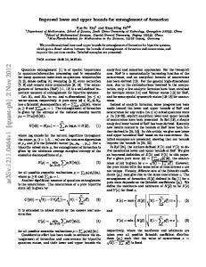
Figure 1: A simple example for the two phases in the heuristic of Liu and Terzi [12]. Phase 1: Anonymize the degree sequence D of the input graph G by increasing the numbers in it such that each resulting number occurs at least k times. Phase 2: Realize the k-anonymized degree sequence D′ as a super-graph of G.

heuristic which, in a nutshell, consists of the following two phases: i) Ignore the graph structure and solve a corresponding number problem and ii) try to transfer the solution from the number problem back to the graph instance. More formally (see Figure 1 for an example), given an instance (G, k), first compute the degree sequence D of G, that is, the multiset of positive integers corresponding to the vertex degrees in G. Then, Phase 1 consists of k-anonymizing the degree sequence D (each number occurs at least k times) by a minimum amount of increments to the numbers in D resulting in D′ . In Phase 2, try to realize the k-anonymous sequence D′ as a supergraph of G, meaning that each vertex gets a demand, which is the difference of its degree in D′ compared to D, and then a “realization” algorithm adds edges to G such that for each vertex the amount of incident new edges equals its demand. Note that, since the minimum “k-anonymization cost” of the degree sequence D (sum over all demands) is always a lower bound on the k-anonymization cost of G, the above described algorithm, if successful when trying to realize D′ in G, optimally solves the given Degree Anonymization instance. Related Work. We only discuss work on Degree Anonymization directly related to what we present here. Our algorithm framework is based on the two-phase algorithm due to Liu and Terzi [12] where also the model of graph (degree-)anonymization has been introduced. Other models of graph anonymization have been studied as well, see Zhou and Pei [19] (studying the neighborhood of vertices) and Chester et al. [4] (anonymizing vertex subsets). We refer to Zhou et al. [20] for a survey on anonymization techniques for social networks. Degree Anonymization is NP-hard for constant k ≥ 2 and it is W[1]-hard (presumably not fixed-parameter tractable) with respect to the parameter size of a solution size [11]. On the positive side, there is polynomial-size kernel (efficient and effective preprocessing) with respect to the maximum degree of the input graph [11]. Lu et al. [13] and Casas-Roma et al. [3] designed and evaluated heuristic algorithms that are our reference points for comparing our results. Our Contributions. Based on the two-phase approach of Liu and Terzi [12] we significantly improve the lower bound provided in Phase 1 and provide a simple heuristic for new upper bounds in Phase 2. Our algorithms are designed to deal with large-scale real world social networks (up to half a million vertices) and exploit some common features of social networks such as the power-law degree distribution [1]. For Phase 1, we provide a new dynamic programming algorithm of k-anonymizing a degree sequence D “improving” the previous running time O(nk) to O(∆k 2 s). Note that maximum degree ∆ is in our considered instances about 500 times smaller than the number of vertices n. We also implemented a data reduction rule which leads to significant speedups of the dynamic program. We study two different cases to obtain upper bounds. If one of the degree sequences computed in Phase 1 is realizable, then this gives an optimal upper bound and otherwise we heuristically look for “near” realizable degree sequences. For Phase 2 we evaluate the already known “local exchange” heuristic [12] and provide some theoretical justification of its quality. We implemented our algorithms and compare our upper bounds with a heuristic of Lu et al. [13], called clustering-heuristic in the following. Our empirical evaluation demonstrates that in about 26% of the real-world instances the lower bound matches the upper bound and in the remaining instances our heuristic upper bound is on average 40% smaller than the one provided by the clustering-heuristic. However, this comes at a cost of increased running time: the clusteringheuristic could solve all instances within 15 seconds whereas there are a few instances where our 2

algorithms could not compute an upper bound within one hour. Due to the space constraints, all proofs and some details are deferred to an appendix.

2

Preliminaries

We use standard graph-theoretic notation. All graphs studied in this paper are undirected and simple without self-loops and multi-edges. For a given graph G = (V, E) with vertex set V and edge set E we set n := |V | and m := |E|. Furthermore, by degG (v) we denote the degree of a vertex v ∈ V in G and ∆G denotes the maximum degree in G. For 0 ≤ d ≤ ∆G let BdG := {v ∈ V | degG (v) = d} be the block of degree d, that is, the set of all vertices with degree d in G. Thus, being k-anonymous is equivalent to each block being of size either zero or at least k. For a set S of edges with endpoints in a graph G, we denote by G + S the graph that results from inserting all edges from S into G. We call S an edge insertion set for G, and if G + S is k-anonymous, then it is an k-insertion set. A degree sequence D is a multiset of positive integers and ∆D denotes its maximum value. The degree sequence of a graph G with vertex set V = {v1 , . . . , vn } is DG := {degG (v1 ), . . . , degG (vn )}. For a degree sequence D, we denote by bd how often value d occurs in D and we set B = {b0 , . . . , b∆D } to be the block sequence of D, that is, B is just the list of the block sizes of G. Clearly, the block sequence of a graph G is the block sequence of G’s degree sequence. The block sequence can be viewed as a compact representation of a degree sequence (just storing the amount of vertices for each degree) and we use these two representations of vertex degrees interchangeably. Equivalently to graphs, a block sequence is k-anonymous if each value is either zero or at least k and a degree sequence is k-anonymous if its corresponding block sequence is k-anonymous. Let D = {d1 , . . . , dn } and D′ = {d′1 , . . . , d′n }Pbe two degree sequences with corresponding block n sequences B and B ′ . We define kBk = |D| = i=1 di . We write D′ ≥ D and B ′ = B if for both degree sequences—sorted in ascending order—it holds that d′i ≥ di for all i. Intuitively, this captures the interpretation “D′ can be obtained from D by increasing some values”. If D′ ≥ D, then (for sorted degree sequences) we define the degree sequence D′ − D = {d′1 − d1 , . . . , d′n − dn } and set B ′ ⊖ B to be its block sequence. We omit sub- and superscripts if the graph is clear from the context.

3

Description of the Algorithm Framework

In this section we present the details of our algorithm framework to solve Degree Anonymization. We first provide a general description how the problem is split into several subproblems (basically corresponding to the two-phase approach of Liu and Terzi [12]) and then describe the corresponding algorithms in detail.

3.1

General Framework Description

We first provide a more formal description of the two-phase approach due to Liu and Terzi [12] and then describe how we refine it: Let (G = (V, E), k) be an input instance of Degree Anonymization. Phase 1: For the degree sequence D of G, compute a k-anonymous degree sequence D′ such that D′ ≥ D and |D − D′ | is minimized. Phase 2: Try to realize D′ in G, that is, try to find an edge insertion set S such that the degree sequence of G + S is D′ . The minimum k-anonymization cost of D, formally |D′ − D|/2, is a lower bound on the number of edges in a k-insertion set for G. Hence, if succeeding in Phase 2 to realize D′ , then a minimum-size k-insertion set S for G has been found.

3

B ′ = {0, 3, 0, 5, 0, 0, 2}

B = {0, 3, 1, 4, 0, 1, 1}

Figure 2: A graph (left side) with block sequence B that can be 2-anonymized by adding one edge (right side) resulting in B′ . Another 2-anonymous block sequence (also of cost two) that will be found by the dynamic programming is B′′ = {0, 2, 2, 4, 0, 0, 2}. The realization of B′′ in G would require to add an edge between a degree-five vertex (there is only one) and a degree-one vertex, which is impossible.

Liu and Terzi [12] gave a dynamic programming algorithm which exactly solves Phase 1 and they provided the so-called local exchange heuristic algorithm for Phase 2. If Phase 2 fails, then the heuristic of Liu and Terzi [12] relaxes the constraints and tries to find a k-insertion set yielding a graph “close” to D′ . We started with a straightforward implementation of the dynamic programming algorithm and the local exchange heuristic. We encountered the problem that, even when iterating through all minimum k-anonymous degree sequences D′ , one often fails to realize D′ in Phase 2. More importantly, we observed the difficulty that iterating through all minimum sequences is often to time consuming because the same sequence is recomputed multiple times. This is because the dynamic program iterates through all possibilities to choose “sections” of consecutive degrees in the (sorted) degree sequence D that end up in the same block in D′ . These sections have to be of length at least k (the final block has to be full) but at most 2k − 1 (longer sections can be split into two). However, if there is a huge block B (of size ≫ 2k) in D, then the algorithm goes through all possibilities to split B into sections, although it is not hard to show that at most k − 1 degrees from each block are increased. Thus, different ways to cut these degrees into sections result in the same degree sequence. We thus redesigned the dynamic program for Phase 1. The main idea is to consider the block sequence of the input graph and exploiting the observation that at most k − 1 degrees from a block are increased in a minimum-size solution. Therefore, we avoid to partition one block into multiple sections and the running time dependence on the number of vertices n can be replaced by the maximum degree ∆, yielding a significant performance increase. We also improved the lower bound provided by D′ − D on the k-anonymization cost of G. To this end, the basic observation was that while trying to realize one of the minimum k-anonymous sequences D′ in Phase 2 (failing in almost all cases), we encountered that by a simple criterion on the sequence D′ − D one can even prove that D′ is not realizable in G. That is, a k-insertion set S for G corresponding to D′ would induce a graph with degree sequence D′ − D. Hence, the requirement that there is a graph with degree sequence D′ − D is a necessary condition to realize D′ in G in Phase 2. Thus, for increasing cost c, by iterating through all k-anonymous sequences D′ with |D′ − D| = c and excluding the possibility that D′ is realizable in G by the criterion on D′ − D, one can step-wisely improve the lower bound on the k-anonymization cost of G. We apply this strategy and thus our dynamic programming table allows to iterate through all k-anonymous sequences D′ with |D′ − D| = c. Unfortunately, even this criterion might not be sufficient because the already present edges in G might prevent the insertion of a k-insertion set which corresponds to D′ − D (see Figure 2 for an example). We thus designed a test which not only checks whether D′ − D is realizable but also takes already present edges in G into account while preserving that |D′ − D| is a lower bound on the k-anonymization cost of G. With this further requirement on the resulting sequences D′ of Phase 1, in our experiments we observe that Phase 2 of realizing D′ in G is in 26 % of the real-world instances successful. Hence, 26 % of the instances can be solved optimally. See Subsection 3.2 for a detailed description of our algorithm for Phase 1. For Phase 2 the task is to decide whether a given k-anonymization D′ can be realized in G. As we will show that this problem is NP-hard, we split the problem into two parts and try to solve each part separately by a heuristic. First, we find a degree-vertex mapping, that is, we assign each 4

degree d′i ∈ D′ to a vertex v in G such that d′i ≥ degG (v). Then, the demand of vertex v is set to d′i − degG (v). Second, given a degree-vertex mapping with the corresponding demands we try the find an edge insertion set such that the number of incident new edges for each vertex is equal to its demand. While the second part could in principle be done optimally in polynomial-time by solving an f -factor problem [11], we show that already a heuristic refinement of the “local exchange” heuristic due to Liu and Terzi [12] is able to succeed in most cases. Thus, theoretically and also in our experiments, the “hard part” is to find a good degree-vertex mapping. Roughly speaking, the difficulties are that, according to D′ , there is more than one possibility of how many vertices from degree i are increased to degree j > i. Even having settled this it is not clear which vertices to choose from block i. See Subsection 3.3 for a detailed description of our algorithm for Phase 2.

3.2

Phase 1: Exact k-Anonymization of Degree Sequences

We start with providing a formal problem description of k-anonymizing a degree sequence D and describe our dynamic programming algorithm to find such sequences D′ . We then describe the criteria that we implemented to improve the lower bound |D′ − D|. Basic Number Problem. The decision version of the degree sequence anonymization problem reads as follows. k-Degree Sequence Anonymity (k-DSA) Input: A block sequence B and integers k, s ∈ N. Question: Is there a k-anonymous block sequence B ′ = B such that kB ′ ⊖ Bk = s? The requirements on B ′ in the above definition ensure that B ′ can be obtained by performing exactly s many increases to the degrees in B. Liu and Terzi [12] give a dynamic programming algorithm that solves k-DSA optimally in O(nk) time and space. Here, besides using block instead of degree sequences, we added another dimension to the dynamic programming table storing the cost of a solution. Lemma 1. k-Degree Sequence Anonymity can be solved in O(∆ · k 2 · s) time and O(∆ · k · s) space. Proof. Let (B, k, s) be an instance of k-Degree Sequence Anonymity. We describe a dynamic programming algorithm. The algorithm maintains a table T where the entry T [i, t, c] with 0 ≤ i ≤ ∆, 0 ≤ c ≤ s, and 0 ≤ t < 2k is true if and only if the block sequence B(i) = {B0 , . . . , Bi } minus the last t degrees can be k-anonymized with cost exactly c. Formally, B(i) minus the last t degrees is the block sequence B ′ (i) corresponding to the degree sequence D that is obtained from DB(i) by removing the t highest degrees. For we 0 ≤ i < ∆ we denote by cost(i, t) the cost to increase the last t degrees in B(i) to i + 1. We compute T [i, t, c] with the following recursion.   c = 0 ∧ (|B0 | − t = 0 ∨ |B0 | − t ≥ k), i=0   ∃t′ ∈ N : k − (|B | − t) ≤ t′ < 2k ∧ i T [i, t, c] = |Bi | > t  T [i − 1, t′ , c − cost(i − 1, t′ )] = true,    T [i − 1, t − |Bi |, c], |Bi | ≤ t. The entry T [∆, 0, s] is true if and only if (B, k, s) is a yes-instance. We compute the cost-function in a preprocessing step in O(∆ · k 2 ) time and O(∆ · k) space. Having computed the cost-function each table entry in T can be computed in O(k) time. As there are ∆ · k · s table entries, the overall running time is O(∆ · k 2 · s). As to the correctness, observe that if i = 0 in the recursion, then c has to be positive and exactly t degrees of block B0 have to be increased by at least one, which is possible only if |B0 | − t = 0 or |B0 | − t ≥ k. If i > 0 and |Bi | ≤ t, then clearly all degrees in the block Bi have to be increased. If i > 0 and |Bi | > t, then there remain some degrees in the block Bi . Thus, the block has to be of size at least k implying that at least min(0, k − (|Bi | − t)) degrees have to be 5

added to Bi . Furthermore, adding more than 2k vertices is not necessary, as in this case we would add only k vertices to ensure that both the blocks Bi and Bi−1 are large enough, that is, |Bi′ | ≥ k ′ and |Bi−1 | ≥ k. The correctness now follows from the fact that the recursion tries all possibilities for the value t′ between min(0, k − (|Bi | − t)) and 2k. There might be multiple minimum solutions for a given k-DSA instance while only one of them is realizable, see Figure 2 for an example. Hence, instead of just computing one minimum-size solution, we iterate through these minimum-size solutions until one solution is realizable or all solutions are tested. Observe that there might be exponentially many minimum-size solutions: In the block sequence B = {0, 3, 1, 3, 1, . . . , 3, 1, 3}, for k = 2, each subsequence 3, 1, 3 can be either changed to 2, 2, 3 or to 3, 0, 4. We use a data reduction rule (see end of this subsection) to reduce the amount of considered solutions in such instances. Criteria on the Realizability of k-DSA Solutions. A difficulty in the solutions provided by Phase 1, encountered in our preliminary experiments and as already observed by Lu et al. [13] on a real-world network, is the following: If a solution increases the degree of one vertex v by some amount, say 100, and the overall number of vertices with increased degree is at most 100, then there are not enough neighbors for v to realize the solution. We overcome this difficulty as follows: For a k-DSA-instance (B, k) and a corresponding solution B ′ , let S be a k-insertion set for G such that the block sequence of G + S is B ′ . By definition, the block sequence of the graph induced by the edges S is B ′ ⊖ B. Hence, it is a necessary condition (for success in Phase 2) that B ′ ⊖ B is a realizable block sequence, that is, there is a graph with block sequence B ′ ⊖ B. Tripathi os-Gallai characterization of and Vijay [18] have shown that it is enough to check to following Erd˝ realizable degree sequence just once for each block. Lemma 2 ([8]). Let D =P {d1 , . . . , dn } be a degree sequence sorted in descending order. Then D is realizable if and only if ni=1 di is even and for each 1 ≤ r ≤ n − 1 it holds that r X

di ≤ r(r − 1) +

n X

min(r, di ).

(1)

i=r+1

i=1

We call the characterization provided by Lemma 2 the Erd˝ os-Gallai test. Unfortunately, there are k-anonymous sequences D′ , passing the Erd˝ os-Gallai test, but still or not realizable in the input graph G (see Figure 2 for an example). We thus designed an advanced version of the Erd˝ os-Gallai test that takes the structure of the input graph into account. To explain the basic idea behind, we first discuss how Inequality (1) in Lemma 2 can be interpreted: Let V r be the set of vertices corresponding to the first r degrees. The left-hand side sums over the degrees of all vertices in V r . This amount has to be at most as large as the number of edges (counting each twice) that can be “obtained” by making V r a clique (r(r − 1)) and the maximum number of edges to the vertices in V \ V r (a degree-di vertex has at most min{di , r} neighbors in V r ). The reason why the Erd˝ os-Gallai test might not be sufficient to determine whether a sequence can be realized in G is that it ignores the fact that same vertices in V r might be already adjacent in G and it also ignores the edges between vertices in V r and V \ V r . Hence, the basic idea of our advanced Erd˝ os-Gallai test is, whenever some of the vertices corresponding to the degrees can be uniquely determined, to subtract the corresponding number of edges as they cannot contribute to the right-hand side of Inequality (1). While the difference between using just the Erd˝ os-Gallai test and the advanced Erd˝ os-Gallai test resulted in rather small differences for the lower bound (at most 10 edges), this small difference was important for some of our instances to succeed in Phase 2 and to optimally solve the instance. We think that further improving the advanced Erd˝ os-Gallai test is the best way to improve the rate of success in Phase 2. Complete Strategy for Phase 1. With the above described restriction for realizable k-anonymous degree sequences, we finally arrive at the following problem for Phase 1, stated in the optimization form we solve:

6

Realizable k-Degree Sequence Anonymity (k-RDSA) Input: A degree sequence B and an integer k ∈ N. Task: Compute all k-anonymous degree sequences B ′ such that B ′ = B, kB ′ ⊖ Bk is minimum, and B ′ ⊖ B is realizable. Our strategy to solve k-RDSA is to iterate (for increasing solution size) through the solutions of k-DSA and run for each of them the advanced Erd˝ os-Gallai test. Thus, we step-wisely increase the respective lower bound B ′ − B until we arrive at some B ′ passing the test. Then, for each solution of this size we test in Phase 2 whether it is realizable (if so, then we found an optimal solution). If the realization in Phase 2 fails, then, for each such block sequence B ′ , we compute how many degrees have to be “wasted” in order to get a realizable sequence. Wasting means to greedily increase some degrees in B ′ (while preserving k-anonymity) until the resulting degree sequence is realizable in the input graph. The cost B ′ − B plus the amount of degrees needed to waste in order to realize B ′ is stored as an upper-bound. A minimum upper-bound computed in this way is the result of our heuristic. Due to the power law degree distribution in social networks, the degree of most of the vertices is close to the average degree, thus one typically finds in such instances two large blocks Bi and Bi+1 containing many thousands of vertices. Hence, “wasting” edges is easy to achieve by increasing degrees from Bi by one to Bi+1 (this is optimal with respect to the Erd˝ os-Gallai characterization). For the case that two such blocks cannot be found, as a fallback we also implemented a straightforward dynamic programming to find all possibilities to waste edges to obtain a realizable sequence. Remark. We do not know whether the decision version of k-RDSA (find only one such solution B ′ ) is polynomial-time solvable and resolving this question remains as challenge for future research. Data Reduction Rule. In our preliminary experiments we observed that for some instances we could not finish Phase 1 even for k = 2 within a time limit of one hour. Our investigations revealed that this is mainly due to the frequent occurrence of the following “pattern” within three consecutive blocks: The first block i and the third block i + 2 are each of size at least 2k − 1 and the middle block consists of k − 1 degrees. For example, for k = 2 consider the consecutive blocks 4, 1, 4. The details of the dynamic program (see Section 3.2) show that in any solution for the entire block sequence block i and i + 2 stay full and either block i + 1 is filled by the degrees from block i or they are increased to block i + 2. In our example this means that the solution is either 4, 0, 4 or 3, 2, 4 (block i + 2 could contain less degrees but at least k). Then, if this pattern occurs multiple, say x, times, then there 2x different solutions in Phase 1. However, as can be observed in our example, with respect to the Erd˝ os-Gallai test whether the resulting sequence is realizable both solutions, 4, 0, 4 and 3, 2, 4, are equivalent because they increase just one degree by one. The general idea of our data reduction rule is to find these patterns where the first and last block are “large” enough to guarantee that the degrees of preceding blocks are not increased to the middle of the pattern and it is not necessary to increase something from the middle of the pattern to succeeding blocks. Hence, the middle of the pattern can be solved “independently” from preceding and succeeding blocks and if there is a minimum solution which is “Erd˝os-Gallaioptimal” (increasing degrees by at most one), then it is safe to take one of them for the middle of the pattern. Formally, our data reduction rule, generalizing the above ideas, is as follows. Rule 1. Let (B, k) be an instance of k-RDSA. If there is a block Bi in B with bi ≥ k, a sequence of P blocks Bj , Bj + 1, . . . , Bj+t such that j+t l=j bl ≥ (t + 1)k + k − 1 and bl ≥ k for all l ∈ {j, . . . , j + t}, ′ and if there is minimum-size k-anonymization Bi,j of the block sequence Bi,j = Bi , Bi+1 , . . . , Bj ′ ′ such that i) all blocks l for l ≥ 2 in Bi,j ⊖ Bi,j are empty and ii) block zero in Bi,j is of size at ′ least k, then substitute in B the subsequence Bi,j by Bi,j . In our implementation of Rule 1 we use our dynamic programming algorithm (with disabled ′ Erd˝ os-Gallai test) to check whether there is a k-anonymization Bi,j for Bi,j fulfilling the required properties. 7

3.3

Phase 2: Realizing a k-Anonymous Degree Sequence

Let (G, k) be an instance of Degree Anonymization and let B be the block sequence of G. In Phase 1 a k-anonymization B ′ of B is computed such that B ′ = B. In Phase 2, given G and B ′ , the task is to decide whether there is a set S of edge insertions for G such that the block sequence of G + S is equal to B ′ . We call this the Degree Realization problem and first prove that it is NP-hard. Theorem 1. Degree Realization is NP-hard even on cubic planar graphs. Proof. We prove the NP-hardness by a reduction from the Independent Set problem: Given a graph G = (V, E) and an integer ℓ, decide whether there is a set of at least ℓ pairwise non-adjacent vertices in G. Independent Set remains NP-hard in cubic planar graphs [10, GT20]. The reduction, which is similar to those proving that Degree Anonymization remains NPhard on 3-colorable graphs [11, Theorem 1], is as follows: Let G be a cubic planar and ℓ an integer that together form an instance of Independent Set. The block sequence of the n-vertex graph G is B = {0, 0, 0, n}. We set B ′ = {0, 0, 0, n − ℓ, 0, . . . , 0, ℓ} | {z } ℓ−2

and next prove that the Degree Realization-instance (G, B ′ ) is a yes-instance if and only if (G, ℓ) is a yes-instance for Independent Set. If there is an independent set S (pairwisely non-adjacent vertices) of size ℓ in G, then adding all edges between the vertices in S (making them a clique), results in a graph whose block sequence in B ′ . Reversely, in a realization of B ′ in G, there are exactly ℓ vertices whose degree has been increased by ℓ − 1. Hence, these vertices form a clique, implying that they are independent in G. We remark that from the details of the proof of Theorem 1 [11], it follows that Degree Realization is NP-hard even in case that B ′ is a k-anonymized sequence such that kB ′ − Bk is minimum.

We next present our heuristics for solving Degree Realization. First, we find a degreevertex mapping, that is, for D′ = d′1 , . . . , d′n being the degree sequence corresponding to B ′ , we assign each value d′i to a vertex v in G such that d′i ≥ degG (v) and set D(v), the demand of v, to d′i − degG (v). Second, we try to find, mainly by the local exchange heuristic, an edge insertion set S such that in G + S the amount of incident new edges for each vertex v is equal to its demand D(v). The details in the proof of Theorem 1 indeed show that already finding a realizable degree-vertex mapping is NP-hard. This coincides with our experiments, as there the “hard part” is to find a good degree-vertex mapping and the local exchange heuristic is quite successful in realizing it (if possible). Indeed, we prove that “large” solutions can be always realized by it: is always realizable by the local exchange heuristic in a maxiTheorem 2. A demand function DP mum degree-∆ graph G = (V, E) if v∈V D(v) ≥ 20∆4 + 4∆2 . In Appendix A (appendix) we give a detailed description of our algorithms for Phase 2 and formally prove the above theorem.

4

Experimental Results

Implementation Setup. All our experiments are performed on an Intel Xeon E5-1620 3.6GHz machine with 64GB memory under the Debian GNU/Linux 6.0 operating system. The program is implemented in Java and runs under the OpenJDK runtime environment in version 1.7.0 25. The time limit for one instance is set to one hour per k-value and we tested for k = 2, 3, 4, 5, 7, 10, 15, 20, 30, 50, 100, 150, 200. After reaching the time limit, the program is aborted and the upper and lower bounds computed so far by the dynamic program for Phase 1 are returned. The source code is freely available.2 2 http://fpt.akt.tu-berlin.de/kAnon/

8

Table 1: Experimental results on real-world instances. We use the following abbreviations: CH for clustering-heuristic of Lu et al. [13], OH for our upper bound heuristic, OPT for optimal value for the Degree Anonymization problem, and DP for dynamic program for the k-RDSA problem. If the time entry for DP is empty, then we could not solve the k-RDSA instance within one-hour and the DP bounds display the lower and upper bounds computed so far. If OPT is empty, then either the k-RDSA solutions could not be realized or the k-RDSA instance could not be solved within one hour.

graph k coAuthorsDBLP 2 (n ≈ 2.9 · 105 , 5 m ≈ 9.7 · 105 , 10 ∆ = 336) 100 coPapersCiteseer 2 (n ≈ 4.3 · 105 , 5 m ≈ 1.6 · 107 , 10 ∆ = 1188) 100 coPapersDBLP 2 (n ≈ 5.4 · 105 , 5 m ≈ 1.5 · 107 , 10 100 ∆ = 3299)

solution size DP bounds time (in seconds) CH OH OPT lower upper CH OH DP 97 62 61 61 1.47 0.08 0.043 531 321 317 317 317 1.41 0.29 26.774 1,372 893 869 869 1.03 0.48 1.58 21,267 15,050 10,577 11,981 1.13 885.79 203 80 78 78 9.9 0.1 0.394 998 327 327 327 327 10.32 0.19 0.166 2,533 960 960 960 960 8.83 0.74 0.718 51,456 22,030 22,007 22,007 22,007 5.97 263.95 264.553 1,890 1,747 950 1,733 11.28 2.13 9,085 8,219 4,414 8,121 10.66 28.83 19,631 17,571 9,557 17,328 9.95 149.56 258,230 128,143 233,508 22.16

Real-World Instances. We considered the five social networks from the co-author citation category in the 10th DIMACS challenge [6]. We compared the results of our upper bounds against an implementation of the clusteringheuristic provided by Lu et al. [13] and against the lower bounds given by the dynamic program. Our algorithm could solve 26% of the instances to optimality within one hour. Interestingly, our exact approach worked best with the coPapersCiteseer graph from the 10th DIMACS challenge although this graph was the largest one considered (in terms of n + m). For all tested values of k except k = 2, we could optimally k-anonymize this graph and for k = 2 our upper bound heuristic is just two edges away from our lower bound. The coAuthorsDBLP graph is a good representative for the results on the DIMACS-graphs, see Table 1: A few instances could be solved optimally and for the remaining ones our heuristic provides a fairly good upper bound. One can also see that the running times of our algorithms increase (in general) exponentially in k. This behavior captures the fact that our dynamic program for Phase 1 iterates over all minimal solutions and for increasing k the number of these solutions increases dramatically. Our heuristic also suffers from the following effect: Whereas the maximum running time of the clustering-heuristic heuristic was one minute, our heuristic could solve 74% of the instances within one minute and did not finish within the one-hour time limit for 12% of the tested instances. However, the solutions produced by our upper bound heuristic are always smaller than the solutions provided by the clustering-heuristic, on average the clustering-heuristic results are 72% larger than the results of our heuristic. Random Instances. We generated random graphs according to the model by Barab´ asi–Albert [1] using the implementation provided by the AGAPE project [2] with the JUNG library3 . Starting with m0 = 3 and m0 = 5 vertices these networks evolve in t ∈ {400, 800, 1200, . . ., 34000} steps. In each step a vertex is added and made adjacent to m0 existing vertices where vertices with higher degree have a higher probability of being selected as neighbor of the new vertex. In total, we created 170 random instances. Our experiments reveal that the synthetic instances are particular hard. For example, even for k = 2 and k = 3 we could only solve 14% of the instances optimal although our dynamic program produces solutions for Phase 1 in 96% of the instances. For higher values of k the results are even worse (for example zero exactly solved instances for k = 10). This indicates that the current lower bound provided by Phase 1 needs further improvements. However, the upper bound 3 http://jung.sourceforge.net/

9

800 solution size

solution size

600 400 200

600 400 200 0

0 0

1

2

0

3

n

·10

1

4

2

3 ·104

n

1,000

solution size

solution size

1,500

500

1,000 500 0

0 0

1

2 n

3

0 ·104

1

2 n

3 ·104

Figure 3: Comparison of our heuristic (always the light blue line without marks) with the clusteringheuristic (always the light red line with little star as marks) on random data with different parameters: Top row is for k = 2, bottom row for k = 3; the left column is for m0 = 3, and the right column for m0 = 5. The linear, solid dark red line and dash-dotted blue line are linear regressions of the corresponding data plot. One can see that our heuristic produces always smaller solutions.

provided by our heuristic are not far away: On average the upper bound is 3.6% larger than the lower bound and the maximum is 15%. Further enhancing the advanced Erd˝ os-Gallai test seem to be the most promising step towards closing this gap between lower and upper bound. Comparing our heuristic with the clustering-heuristic reveal similar results as for real-world instances. Our heuristic always beats the clustering-heuristic in terms of solution size, see Figure 3 for k = 2 and k = 3. We remark that for larger values of k the running time of the heuristic increases dramatically: For k = 30 our algorithm provides upper bounds for 96% of the instances, whereas for k = 150 this value drops to 18%.

5

Conclusion

We have demonstrated that our algorithm framework is suitable to solve Degree Anonymization on real-world social networks. The key ingredients for this is an improved dynamic programming for the task to k-anonymize degree sequences together with certain lower bound techniques, namely the advanced Erd˝ os-Gallai test. We have also demonstrated that the local exchange heuristic due to Liu and Terzi [12] is a powerful algorithm for realizing k-anonymous sequences and provided some theoretical justification for this effect. The most promising approach to speedup our algorithm and to overcome its limitations on the considered random data, is to improve the lower bounds provided by the advanced Erd˝ os-Gallai test. Towards this, and also to improve the respective running times, one should try to answer the question whether one can find in polynomial-time a minimum k-anonymization D′ of a given degree sequence D such that D′ − D is realizable.

10

Bibliography [1] A. Barab´ asi and R. Albert. Emergence of scaling in random networks. Science, 286(5439): 509–512, 1999. 2, 9 [2] P. Berthom´e, J.-F. Lalande, and V. Levorato. Implementation of exponential and parametrized algorithms in the AGAPE project. CoRR, abs/1201.5985, 2012. 9 [3] J. Casas-Roma, J. Herrera-Joancomart´ı, and V. Torra. An algorithm for k-degree anonymity on large networks. In Proc. ASONAM’13, pages 671–675. ACM Press, 2013. 1, 2 [4] S. Chester, J. Gaertner, U. Stege, and S. Venkatesh. Anonymizing subsets of social networks with degree constrained subgraphs. In Proc. ASONAM’12, pages 418–422. IEEE Computer Society, 2012. 1, 2 [5] R. Diestel. Graph Theory, volume 173 of Graduate Texts in Mathematics. Springer, 4th edition, 2010. 13 [6] DIMACS’12. Graph partitioning and graph clustering. 10th DIMACS challenge, 2012. URL http://www.cc.gatech.edu/dimacs10/. Accessed April 2012. 9 [7] D. Easley and J. Kleinberg. Networks, Crowds, and Markets. Cambridge University Press, 2010. 1 [8] P. Erd˝ os and T. Gallai. Graphs with prescribed degrees of vertices (in Hungarian). Math. Lapok, 11:264–274, 1960. 6 [9] B. C. M. Fung, K. Wang, R. Chen, and P. S. Yu. Privacy-preserving data publishing: A survey of recent developments. ACM Computing Surveys, 42(4):14:1–14:53, 2010. 1 [10] M. R. Garey and D. S. Johnson. Computers and Intractability: A Guide to the Theory of NP-Completeness. Freeman, 1979. 8 [11] S. Hartung, A. Nichterlein, R. Niedermeier, and O. Such´ y. A refined complexity analysis of degree anonymization in graphs. In Proc. 40th ICALP, volume 7966 of LNCS, pages 594–606. Springer, 2013. 1, 2, 5, 8, 13 [12] K. Liu and E. Terzi. Towards identity anonymization on graphs. In Proc. SIGMOD ’08, pages 93–106. ACM, 2008. 1, 2, 3, 4, 5, 10, 13 [13] X. Lu, Y. Song, and S. Bressan. Fast identity anonymization on graphs. In Proc. DEXA’12, Part I, volume 7446 of LNCS, pages 281–295. Springer, 2012. 1, 2, 6, 9, 17 [14] P. Samarati. Protecting respondents identities in microdata release. IEEE Transactions on Knowledge and Data Engineering, 13(6):1010–1027, 2001. 1 [15] P. Samarati and L. Sweeney. Generalizing data to provide anonymity when disclosing information. In Proc. PODS’98, pages 188–188. ACM, 1998. 1 [16] L. Sweeney. k-anonymity: A model for protecting privacy. International Journal of Uncertainty, Fuzziness and Knowledge-Based Systems, 10(5):557–570, 2002. 1 [17] B. Thompson and D. Yao. The union-split algorithm and cluster-based anonymization of social networks. In Proc. 4th ASIACCS’09, pages 218–227. ACM, 2009. 1 [18] A. Tripathi and S. Vijay. A note on a theorem of Erd¨ os & Gallai. Discrete Math., 265(1-3): 417–420, 2003. 6 [19] B. Zhou and J. Pei. The k-anonymity and l-diversity approaches for privacy preservation in social networks against neighborhood attacks. Knowledge and Information Systems, 28(1): 47–77, 2011. 2 [20] B. Zhou, J. Pei, and W. Luk. A brief survey on anonymization techniques for privacy preserving publishing of social network data. ACM SIGKDD Explorations Newsletter, 10(2):12–22, 2008. 2

11

B ′ = {0, 15, 0, 2, 2, 2, 0, 0, 0, 3}

B = {0, 15, 0, 3, 2, 1, 0, 2, 0, 1}

Figure 4: Our smallest example where “jumps” are necessary to obtain a minimum-size solution. The only minimum solution to 2-anonymize the left graph is to add the bold edges in the right graph. Observe that, although there are two degree-four vertices in the graph, the solution lifts a degree-three vertex to degree five, that is, there is a “jump” of two.

A

Detailed Description of the Algorithms for Phase 2: Realizing the k-anonymous degree sequence

Phase 2.1: Finding a Degree-Vertex Mapping. Given a graph G with its block sequence B and a k-anonymous block sequence B ′ = B, the two main difficulties that arise when trying to find a best possible (realizable) degree-vertex mapping for B ′ are as follows: To illustrate to first one, consider to 2-anonymize a graph consisting of two connected components {a, b, c} and {d, e} where each component is just a path. Hence, the block sequence is B = {0, 4, 1} and a minimum solution would be to insert an edge between two degree-one vertices, resulting in the block sequence B ′ = {0, 2, 3}. Given B ′ , a degree-vertex mapping has to choose two degree-one vertices where all but the choice {d, e} leads to a realization. Hence, the basic problem is that a degree-vertex mapping has to choose x many vertices from block i which is of size more than x and thus the assignment is non-unique. In our experiments we observed that this difficulty can be solved satisfactorily by randomly selecting the vertices from the blocks. However, the second difficulty is a more severe problem, also on practical instances. Assume that B = {3, 2, 1} is the block sequence of our input graph (three degree-zero vertices and a path of length two) and the result of Phase 1 is the 2-anonymized block sequence B ′ = {2, 2, 2}. Now, the difficulty arises that there are actually two “interpretations” of B ′ : The first (natural) one would be to increase a degree zero up to one and a degree two up to three. However, the second would be that one degree zero is increased by two up to three. We call this a jump since a degree is increased “over” a non-empty block, while the natural interpretation (making most sense in the majority of the cases) is that a degree is increased to the next non-empty block B and from there, first the vertices originally in B are increased further. While in the example above the second “jump”-interpretation cannot be realized (only one vertex has non-zero demand), Figure 4 illustrates an example where the only realizable degree-vertex mapping has such a jump. In our experiments, against our a-priori intuition, we observed that the k-anonymized sequences B ′ (computed in Phase 1) have typically less than ten “jump blocks” (a jump over these blocks is possible) and for each of these blocks up to five degrees can jump “over” it. Since the number of jump blocks is reasonably small and as we try to realize many degree-vertex mappings for each B ′ (100 in the results presented in Section 4), it turned out that, for increasing α from zero up to the number of jump blocks, iterating through all possibilities to choose α jump blocks is a good choice. Having fixed the jumps, it follows how many degrees from i are increased to j and we randomly (25 trials for each jump configuration) select the appropriate number of vertices from block Bi in G. In total, for each given B ′ from Phase 1 we try to realize 25 · 100 = 2500 degree-vertex mappings. These parameters (25 and 100) have been chosen according to the results in preliminary experiments and seem to be a good compromise between expected success rate and the needed time. Phase 2.2: Realizing a Degree-Vertex Mapping. In the last part of finding a realization of a k-anonymized sequence B ′ in a graph G = (V, E), one is given a degree-vertex mapping which

12

provides a non-negative integer demand for each vertex and the task is to decide whether it is realizable, that is, is there an edge insertion set S such that in G + S the amount of incident new edges for each vertex is equal to its demand. Formally, let D : V → N be the function providing the demand of each vertex. Whether D is realizable can be decided in polynomial-time by solving an f -factor instance and it has been shown that, for the maximum degree ∆ of G, D is always P realizable if v∈V D(v) ≥ (∆2 + 4∆ + 3)2 [11, Lemma 4]. We have implemented a so-called local exchange heuristic by Liu and Terzi [12] which turned out to perform surprisingly well. Indeed, we here present also some theoretical P justification for this, formally proving that basically the same lower bound (as for f -factor) on v∈V D(v) is enough to guarantee that the local exchange heuristic always realizes D. In principle, the local exchange heuristic adds edges between vertices as long as possible to satisfy their demand and if it gets stuck at some point, then it tries to continue by exchanging an already inserted edge. Formally, it works as follows: Let S be the set of new edges which is initialized by ∅. As long as there are two vertices u and v with non-zero demand, check whether the edge {u, v} is insertable, meaning that neither {u, v} ∈ E nor {u, v} ∈ S. If it is insertable, then add {u, v} to S and decrease the demand of u and v by one. If this procedure ends with all vertices having demand zero, then S is an insertion set realizing D. Otherwise, we are left with a set V D of vertices with non-zero demand. If there are two vertices v1 , v2 ∈ V D , then for each edge {u, w} ∈ S check whether the two edges {v1 , u} and {v2 , w} or {v1 , w} and {v2 , v} are insertable. If so, then delete {u, w} from S, insert the two edges that are insertable, and decrease only one vertex v, then it the demand of v1 and v2 by one. In the special case of V D containing P holds that the remaining demand of v is at least two, because v∈V D(v) can be assumed to be even (otherwise it is not realizable). In this case perform the following for each edge {u, w} ∈ S: Check whether {v, u} and {v, w} are insertable and if so, then insert them to S, delete {u, w} from S, and decrease the demand of v by two. We have implemented the local exchange heuristic so that it first randomly tries to add edges and then, if stuck at some point, performs the above P described exchange operations (if possible). We conclude with proofing a certain lower bound on v∈V D(v) which guarantees the success of the local exchange heuristic. As a first step for this, we prove that any demand function can be assumed to require to increase the vertex degrees at most up to 2∆2 . Lemma 3. Any minimum-size k-insertion set for an instance of Degree Anonymization yields a graph with maximum degree at most 2∆2 . Proof. Before proving Lemma 3, we introduce the terms “co-matching” and “co-cycle cover” and prove an observation concerning their existence. A graph G = (V, E) contains a co-matching of size ℓ if G contains a matching of size ℓ, that is, a subset of ℓ non-overlapping edges of G. A perfect co-matching of G is a co-matching of size |V |/2. Analogously, G contains a co-cycle cover if G contains a cycle cover, that is, a subgraph of G with |V | vertices such that each vertex has degree two. We prove the following observation that shows sufficient conditions for the existence of co-matchings and co-cycle covers. Observation 1. Let G = (V, E) be a graph and let V ′ ⊆ V be a vertex subset with |V ′ | ≥ 2∆ + 1. Then, G[V ′ ] contains a co-cycle cover and if |V ′ | is even, then G[V ′ ] contains a perfect co-matching. Proof. Since |V ′ | ≥ 2∆+1, it follows that in G[V ′ ] every vertex has degree at least |V ′ |−∆ ≥ |V |/2. Hence, using Diracs Theorem [5], it follows that G[V ′ ] contains a Hamiltonian cycle C. Thus it contains a co-cycle cover. Additionally, if |V ′ | is even, then it follows that the number of vertices in C is even and, hence, taking every second edge of C results in a perfect matching. ′

We now prove Lemma 3. We consider an instance (G = (V, E), k) of Degree Anonymization. Let S be a minimum-size k-insertion set for G. Suppose the maximum degree in G + S is greater ˜ be the graph that is obtained from G by iterating over all edges in S (in an than 2∆2 . Let G arbitrary order) and adding an edge if it does not increase the maximum degree ∆. Let S˜ ⊆ S be ˜ By definition G ˜ + S˜ is a k-anonymous graph and adding any edge the edges not contained in G.

13

˜ causes a maximum degree of ∆ + 1. Hence, denoting by X ⊆ V (S) ˜ the vertices of from S˜ to G ˜ \ X. Clearly, the vertices degree ∆, each edge in S˜ has at least one endpoint in X. Let Z = V (S) ˜ + S˜ that have degree greater than ∆ are a subset of V (S) ˜ = X ∪ Z. Next, we show how to in G ˜ whose addition to G ˜ results in a k-anonymous graph. construct an edge set of size less than |S| Case 1: |X| ≤ (∆ + 3)∆. Since, each edge in S˜ contains at least one endpoint from X, every vertex in Z is incident to ˜ Hence, the degree of each vertex from Z in G ˜ + S˜ is less than at most (∆ + 3)∆ edges in S. ˜ + S˜ (∆ + 3)∆ + ∆ ≤ 2∆2 . Thus, only the vertices from X can have degree more than 2∆2 in G and each of them is adjacent to at least 2∆2 − (∆ + 3)∆ > ∆2 /2 + 1 vertices from Z. Now for ˜ + S˜ find two non-adjacent neighbors of it in Z, delete the each vertex u of maximum degree in G edges between u and the neighbors and insert an edge between the neighbors. (Observe that the ˜ has maximum degree at most ∆ − 1 and each such vertex u has neighbors always exist, since G 2 at least ∆ /2 + 1 > ∆ − 1 neighbors from Z.) Hence, we get a smaller set of edge additions that ˜ into a k-anonymous graph, implying a contradiction. also transforms G Case 2: |X| > (∆ + 3)∆ ˜ by inserting at most |S| ˜ edges into a k-anonymous graph. We give an algorithm that transforms G ˜ 1. Initialize S ′ by a copy of S˜ and G′ by a copy of G. 2. While there are any two vertices v, u ∈ V (S ′ ) that are non-adjacent and both have degree less than ∆ in G′ , add the edge {u, v} to G′ , delete one edge in S ′ that is incident to v and one that is incident to u. 3. Let Z ′ = {u ∈ Z ∩ V (S ′ ) | degG′ (u) < ∆}. Find a subset of vertices Y ⊆ X such that there is co-matching in G′ from Z ′ to Y such that each vertex in Y is contained in exactly one comatching edge and each vertex z ∈ Z ′ is contained in exactly min{∆, degG+ ˜ S ˜ (z)} − degG′ (z) co-matching edges. Add the edges of this co-matching. To complete the algorithm we distinguish between several cases. Before that, observe that after Step 2 the maximum degree of G′ is still ∆. Additionally, since each vertex in Y ⊆ X is adjacent to only one co-matching edge and each vertex z ∈ Z ′ gets only min{∆, degG+ ˜ S ˜ (z)} − degG′ (z) additional edges, after Step 3 the maximum degree of G′ is ∆+1. As Step 2 is exhaustively applied, Z ′ induces a clique and thus |Z ′ | ≤ ∆. This implies that |Y | < ∆2 . The existence of the set Y follows from the fact that after Step 2 in G′ each vertex in Z ′ is adjacent to at most ∆ − 1 vertices in X and |X| > (∆ + 3)∆. Thus for each vertex z one can pick any min{∆, degG+ ˜ S ˜ (z)} − degG′ (z) non-adjacent vertices for X that are disjoint from those chosen for the others. ˜ + S, ˜ the degree of each Additionally, since all vertices from X have degree larger than ∆ in G ′ ′ ˜ ˜ ˜ + S˜ that have vertex in G is at most as its degree in G + S. Denote by X all vertices in G ′ degree greater than ∆ but are not contained in Y . All vertices in X have degree ∆ in G′ (see ˜ S˜ that have degree greater than ∆ and thus Step 3). Clearly, X ′ ∪Y are exactly the vertices in G+ ′ |X ∪ Y | ≥ k. Furthermore, we do not change the degree of any vertex V \ (X ′ ∪ Y ). Thus, in the following cases it remains to argue that none of the vertices in X ′ ∪ Y damage the k-anonymous constraint and that the new solution adds less edges than the old one. Case 2.1: |X ′ | is even As (X \ Y ) ⊆ X ′ and |Y | ≤ ∆2 it follows that |X ′ | > 3∆. Hence, by Observation 1 there is a perfect co-matching on the vertices in X ′ and inserting the corresponding edges results in a ˜ because k-anonymous graph. The number of corresponding edge additions is less than those in S, ′ ˜ S increases the degree of all vertices in X ∪ Y also at least to ∆ + 1 and for some of them even above 2∆2 . Case 2.2: |X ′ | is odd Case 2.2.1 k < |X ′ ∪ Y |/2 | ′ We increase via a co-matching on 2⌈ k−|Y 2 ⌉ vertices from X the degree of enough vertices to ∆ + 1 such that together with Y there are at least k degree-(∆ + 1) vertices. Observe that, |X ′ | − | 2⌈ k−|Y 2 ⌉ > 2k − |Y | − (k − |Y |) = k and, thus, there are at least k vertices left with degree ∆.

14

Case 2.2.2 k ≥ |X ′ ∪ Y |/2 Case 2.2.2.1 |Y | is even In this case we add the edges of a co-matching on Y and the edges of a co-cycle in X ′ . This results in a k-anonymous graph with maximum degree ∆ + 2. Note that the number of edge additions in this solution to get degree ∆ + 2 for the vertices in X ′ ∪ Y is less ˜ + S˜ the set S˜ contains at least than (∆ + 2) · |X ′ ∪ Y | whereas for G k · (2∆2 − ∆) |X ′ ∪ Y | · (2∆2 − ∆) ≥ 2 4 edges to increase for at least k vertices the degree from at most ∆ to at least 2∆2 . By Observation 1, there exists a co-cycle cover on X ′ since |X ′ | > 3∆. It remains to argue that there is co-matching on Y . This follows from Observation 1 in case of |Y | > 2∆. However, in case of |Y | ≤ 2∆, because of |X| > (∆ + 3)∆ the choice of Y in Step 3 can be easily adjusted to guarantee the existence of such a matching. Case 2.2.2.2 |Y | is odd ˜ + S˜ can contain at most two vertex-degrees Observe that from k ≥ |X ′ ∪ Y |/2 it follows that G that are larger than ∆. We first argue that there cannot be just one vertex-degree greater than ∆. ˜ + S˜ the have degree larger than ∆, say they have Recall that X ′ ∪ Y are exactly the vertices in G ˜ compared to G ˜ + S˜ degree a. We show that the difference in the sum of the vertex degrees from G is an odd number, a contradiction. First, note that the number of edges that are deleted from S˜ in Step 2 is an even number, we ignore them in the following. Second, S˜ also contains edges that increase (as in Step 3) the degree of each vertex z ∈ Z ′ from degG′ (z) to min{∆, degG+ ˜ S ˜ (z)} and they contribute 2|Y | to the sum of the degrees. Additionally, it contributes |X ′ ∪ Y | · (a − ∆) − |Y | to increase the degree of the vertices from ∆ to a (note that minus Y is necessary because these degrees are already counted for the vertices in Z ′ ). Hence, the difference in the sum of the degrees ˜ to G ˜ + S˜ is |Y | + (|X ′ ∪ Y | · (a − ∆)) which is by our assumptions on |X ′ | and |Y | an odd from G number, implying a contradiction. ˜ + S˜ contains two vertex-degrees that are larger than ∆. It remains to consider the case where G ′ ˜ Hence, k = |X ∪ Y |/2. Again we consider the difference in the sum of the vertex-degree from G ′ ˜ ˜ ˜ ˜ to G + S. The vertex set X ∪ Y is partitioned into a set P1 the has degree a1 in G + S and P2 that has degree a2 . Then the difference on the sum of the degrees is 2|Y |+|P1 |(a1 · ∆) + |P2 |(a2 − ∆) − |Y | |Y |+ P1 (a1 − ∆) + |P2 | (a2 − ∆) |{z} | {z } |{z} | {z } odd

odd

odd

even

Since |Y | is odd exactly one of |P1 |(a1 · ∆) or |P2 |(a2 − ∆) has to be an odd number. This implies together with the assumption that |X ′ ∪ Y | = |P1 ∪ P2 | is an even number that both |P1 | and |P2 | are odd numbers. Hence, since k = |X ′ ∪ Y |/2 this implies that k is an odd number. However, in this case we can make G′ k-anonymous by just adding a co-matching on k − |Y | vertices in X ′ . Remark. We strongly conjecture that the bound in Lemma 3 is not tight. The worst example we found is a graph consisting of two disjoint cliques of size ∆ and ∆ + 1, respectively, and setting k = n. The only k-insertion set for this instance makes the whole graph a clique and, thus, doubles the degree. We conjecture that the bound can be improved to 2∆. By Lemma 3 we may assume that the the maximum degree is not forced to increased by more than 2∆2 − ∆. We now have all ingredients to prove that the local exchange heuristic always realizes “large” demand functions. Theorem 3. Let G = (V, E) be a graph with maximum degree ∆ and let D : V → N be a demand function such that maxv∈V D(v) + degG (v) ≤ 2∆2 . The local exchange heuristic always realizes D P if v∈V D(v) ≥ 20∆4 + 4∆2 .

15

Proof. Towards a contradiction, assume that the local exchange heuristic gets stuck at some point such that no edge is insertable and no further exchange operation can be performed. Denote by V D the set of vertices still having a non-zero demand in V D . Let S be the set of new edges already added at this point. We make a case distinction on the size of S and V D . Case 1: |V D | ≥ 2∆2 + 2 In this case consider any vertex v ∈ V D and observe that it cannot have more than 2∆2 neighbors in G and S together. Hence, there is a vertex u ∈ V D such that {v, u} is insertable. Case 2: |S| ≥ 8∆4 Consider first the subcase where V D consists only of one vertex v. Hence, the demand of v is at least two and since no exhange operation is applicable, for all edges {u, w} ∈ S it holds that either {v, u} or {v, w} is not insertable. However, as v can have at most 2∆2 neighbors in G and S together, from the lower bound on S it follows that there is a least one edge {u, w} ∈ S where the exchange operation can be applied. In the last subcase assume that there are two vertices v1 , v2 ∈ V D . Again, as no exchange operation can be applied, for each edge {u, w} ∈ S it holds that either one of the edges {v1 , u} and {v2 , w} or one of {v1 , w} and {v2 , u} is not insertable. However, for vertex v1 (v2 ) it holds that there are less than (2∆2 )2 = 4∆4 edges in S which contain a neighbor of v1 (v2 , resp.). Hence, from |S| ≥ 8∆4 it follows that there is an edge {u, w} in S where each of {u, w} is non-adjacent to each of {v1 , v2 } and thus the exchange operation can be applied. This completes Case 2. P Since the demand of each vertex in V D is at most 2∆2 , from Case 1 and ξ := v∈V D(v) ≥ 20∆4 + 4∆2 it follows that |S| is at least ξ − |V D | · 2∆2 ξ − (2∆2 + 2)2∆2 ≥ ≥ 8∆4 . 2 2 Hence, Case 2 applies and this causes a contradiction to the assumption that the local exhange heuristic got stuck at some point.

B

Appendix: Full experimental results

Further Real-World Instances. Besides the DIMACS instances we consider coauthor networks derived from the DBLP dataset where the vertices represent authors and the edges represent co-authorship in at least one paper. The DBLP-dataset was generated on February 2012 following the documentation from http://dblp.uni-trier.de/xml/. As it turned out that this DBLP graph is too large for our exact approach, we derived the following subnetworks: First, we made the graph sparser by making two vertices adjacent if the corresponding two authors are co-authors in at least two, three or more papers instead of one paper. We denote these graphs by graph thres 1 (originial graph), graph thres 2, . . ., graph thres 5. Second, we just considered papers that appeared in some algorithm engineering or algorithm theory conference (the exact conference list here is: SEA, WEA, ALENEX, ESA, SODA, WADS, COCOON, ISAAC, WALCOM, AAIM, FAW, SWAT) and removed all isolated vertices. The resulting graph is denoted by graphConference.

16

Table 2: Graph parameters of the real world networks.

DIMACS graps

DBLP subgraphs

graph coPapersDBLP coPapersCiteseer coAuthorsDBLP citationCiteseer coAuthorsCiteseer graph thres 01 graph thres 02 graph thres 03 graph thres 04 graph thres 05 graphConference

n 540,486 434,102 299,067 268,495 227,320 715,633 282,831 167,006 112,949 81,519 5,599

m 15,245,729 16,036,720 977,676 1,156,647 814,134 2511,988 640,697 293,796 168,524 107,831 8,492

∆ 3,299 1,188 336 1,318 1,372 804 201 123 88 71 53

Table 3: Full list of experimental results on real-world instances with enabled data reduction. We use the following abbreviations: CH for clustering-heuristic of Lu et al. [13], OH for our upper bound heuristic, OPT for optimal value for the Degree Anonymization problem, and DP for dynamic program for the k-RDSA problem. If the time entry for DP is empty, then we could not solve the k-RDSA instance within one-hour and the DP bounds display the lower and upper bounds computed so far. If OPT is empty, then either the k-RDSA solutions could not be realized or the k-RDSA instance could not be solved within one hour.

coAuthorsCiteseer

citationCiteseer

graph

k 2 3 4 5 7 10 15 20 30 50 100 150 200 2 3 4 5 7 10 15 20 30 50 100 150 200

solution size CH OH OPT 690 458 1,187 704 1,689 1,133 2,508 1,807 3,860 2,698 6,543 4,966 10,491 8,249 15,934 12,778 24,099 19,800 45,257 98,688 154,753 211,427 1,163 1,002 1,002 2,156 1,837 1,836 3,102 2,979 4,413 4,177 6,304 6,021 9,716 9,332 15,843 15,117 21,630 20,745 34,065 32,719 59,251 57,002 122,996 187,977 252,170

DP bounds lower upper 319 457 526 698 805 1,111 1,224 1,756 1,815 2,653 3,174 4,769 5,117 7,931 7,770 12,058 11,835 18,797 22,316 35,986 49,041 81,438 127,994 127,994 174,040 174,040 1,002 1,002 1,836 1,836 2,977 2,977 4,163 4,163 3,701 5,979 9,283 9,283 7,920 14,932 20,584 20,584 32,424 32,424 61,288 171,411 125,946

17

114,512 171,411 226,200

CH 1.49 2.59 1.27 1.64 0.92 1.08 1.15 1.14 1.41 1.4 2.41 5.25 6.78 0.74 0.98 0.98 0.92 0.62 0.95 0.85 1.03 1.34 1.97 3.77 7.95 10.43

time (in seconds) OH DP 0.53 0.43 1.08 4.14 5.01 43.05 77.71 579.94 1,538.03

0.26 0.33 0.97 1.79 3.11 7.42 48.58 68.74 242.24 2,546.24

1.44 85.87 842.96 1,417.36 3,465.51 64.78 1,330.47

graph thres 02

graph thres 01

coPapersDBLP

coPapersCiteseer

coAuthorsDBLP

graph

k 2 3 4 5 7 10 15 20 30 50 100 150 200 2 3 4 5 7 10 15 20 30 50 100 150 200 2 3 4 5 7 10 15 20 30 50 100 150 200 2 3 4 5 7 10 15 20 30 50 100 150 200 2 3 4 5 7 10 15 20 30 50 100 150 200

solution size CH OH 97 62 253 180 344 231 531 321 817 542 1,372 893 2,352 1,549 3,323 2,188 5,381 3,557 9,661 6,700 21,267 15,050 32,932 24,139 45,411 32,925 203 80 394 136 668 231 998 327 1,915 657 2,533 960 5,147 1,847 6,829 2,627 11,667 4,273 22,795 9,312 51,456 22,030 81,101 36,011 113,526 51,379 1,890 1,747 3,418 3,065 6,236 5,551 9,085 8,219 12,166 10,764 19,631 17,571 31,663 28,538 43,637 39,722 70,590 122,378 258,230 401,143 540,505 290 179 748 483 1,154 729 1,621 1,009 2,516 1,638 3,969 2,632 6,461 4,488 8,761 6,127 13,643 9,712 24,471 53,101 82,684 115,553 32 16 111 50 165 80 258 115 392 178 609 288 1,098 514 1,564 784 2,581 1,389 5,094 2,729 11,281 6,764 18,179 11,347 24,950 16,156

OPT 179 317

21,960 136 231 327 657 960 1,845 2,627 4,273 9,311 22,007 35,881 51,361

16 50 80 115 178 288

2,410 5,419 8,709 11,921

DP bounds lower upper 61 61 179 179 230 230 317 317 414 527 869 869 1,481 1,481 2,081 2,081 3,391 3,391 4,744 6,042 10,577 11,981 16,483 16,483 21,960 21,960 78 78 136 136 231 231 327 327 657 657 960 960 1,845 1,845 2,627 2,627 4,273 4,273 9,311 9,311 22,007 22,007 35,881 35,881 51,361 51,361 950 1,733 1,683 3,030 2,996 5,497 4,414 8,121 5,897 10,615 9,557 17,328 15,403 27,991 21,469 39,048 34,714 62,898 60,535 110,295 128,143 233,508 240,068 359,665 268,409 485,386 166 176 372 475 547 714 745 989 1,188 1,600 1,854 2,524 3,152 4,263 4,227 5,731 6,634 9,277 11,958 16,874 37,792 37,792 40,995 59,281 79,952 79,952 16 16 50 50 80 80 115 115 178 178 288 288 502 502 754 754 1,299 1,299 2,410 2,410 5,419 5,419 8,709 8,709 11,921 11,921

18

CH 1.47 1.26 0.82 1.41 0.63 1.03 0.97 0.84 0.75 0.61 1.13 0.63 0.62 9.9 9.66 9.31 10.32 7 8.83 7.96 8.4 7.62 7.48 5.97 5.51 4.71 11.28 11.66 10.36 10.66 8.39 9.95 9.38 10.24 11.2 14.37 22.16 46.44 61.74 7.16 6.76 5.67 5.78 4.54 4.51 4.69 4.35 4.01 3.39 3.19 3.03 3.93 0.78 0.97 0.47 0.88 0.42 0.47 0.45 0.45 0.41 0.38 0.34 0.54 0.83

time (in seconds) OH DP 0.08 0.04 0.06 0.12 0.14 0.26 0.29 26.77 0.16 0.48 1.58 2.62 4.63 7.69 7.64 19.2 2.40 158.36 885.79 801.69 15.38 271.55 11.94 0.1 0.39 0.11 0.13 0.12 0.13 0.19 0.17 0.35 0.36 0.74 0.72 2.17 2.17 4.1 4.13 9.58 9.47 47.5 47.51 263.95 264.55 490.15 487.55 995.8 984.53 2.13 4.75 11.63 28.83 55.55 149.56 729.36 1,372.12

0.24 2.81 0.97 1.89 5.59 14.46 180.11 179.17 577.17

0.03 0.04 0.04 0.05 0.04 0.07 0.5 0.7 3.79 4.13 6.77 17.61 35.33

0.03 0.04 0.04 0.04 0.05 0.06 0.13 0.65 358.02 0.52 1.57 3.11 4.04

citationCiteseer

graphConference

graph thres 05

graph thres 04

graph thres 03

graph

k 2 3 4 5 7 10 15 20 30 50 100 150 200 2 3 4 5 7 10 15 20 30 50 100 150 200 2 3 4 5 7 10 15 20 30 50 100 150 200 2 3 4 5 7 10 15 20 30 50 100 150 200 2 3 4 5 7 10 15 20 30 50 100 150 200

solution size CH OH 38 25 71 45 121 69 166 94 276 154 439 240 763 382 1,015 536 1,668 830 3,100 1,543 7,150 3,476 11,347 6,359 15,349 8,874 28 15 46 25 82 38 85 39 169 77 267 134 481 230 696 323 1,145 548 2,174 1,041 5,177 2,430 8,165 4,071 11,280 6,270 17 9 28 12 51 25 64 31 135 60 207 102 344 176 537 261 919 429 1,791 857 4,248 1,956 6,906 3,214 9,581 4,590 64 58 104 93 192 154 261 216 417 346 690 553 1,122 880 1,630 1,204 2,474 1,872 4,454 3,177 8,506 6,428 15,699 21,267 690 457 1,187 698 1,690 1,119 2,502 1,816 3,864 2,735 6,537 4,882 10,478 8,365 15,889 12,800 24,166 19,988 45,214 98,683 154,753 211,215

OPT 25 68 94

797 1,491 3,380 5,354 7,450 15 25 38 39 77 134 229 548 1,039 2,398 3,813 5,327 8 12 25 31 60 102 174 261 429 856 1,953 3,122 4,375 58 93 154

4,636 7,225 9,942

DP bounds lower upper 25 25 44 44 68 68 94 94 150 150 238 238 374 374 514 514 797 797 1,491 1,491 3,380 3,380 5,354 5,354 7,450 7,450 15 15 25 25 38 38 39 39 77 77 134 134 229 229 321 321 548 548 1,039 1,039 2,398 2,398 3,813 3,813 5,327 5,327 8 8 12 12 25 25 31 31 60 60 102 102 174 174 261 261 429 429 856 856 1,953 1,953 3,122 3,122 4,375 4,375 58 58 93 93 154 154 214 214 344 344 536 536 851 851 1,157 1,157 1,732 1,732 2,694 2,694 4,636 4,636 7,225 7,225 9,942 9,942 311 457 519 698 802 1,111 1,219 1,756 1,814 2,653 3,173 4,769 5,116 7,931 7,769 12,058 11,834 18,797 22,316 35,986 49,040 81,438 77,049 127,994 105,102 174,040

19

CH 0.26 0.29 0.18 0.24 0.18 0.17 0.17 0.16 0.15 0.15 0.15 0.23 0.33 0.11 0.13 0.1 0.11 0.1 0.09 0.09 0.08 0.08 0.08 0.09 0.16 0.2 0.07 0.06 0.06 0.06 0.06 0.06 0.05 0.05 0.05 0.05 0.05 0.1 0.16 0.04 0.01 0.01 0.01 0.01 0.06 0.01 0.01 0.07 0.01 0.04 0.41 0.75 1.69 1.59 1 1.73 0.9 1.04 0.95 0.83 1.28 1.25 2.23 5.31 6.91

time (in seconds) OH 0.02 0.26 0.04 0.03 0.08 0.22 0.73 0.26 0.45 0.44 0.82 4.12 6.57 0.01 0.05 0.03 0.01 0.01 0.03 0.07 0.15 0.03 0.08 0.35 1.2 3.06 0.01 0.01 0.01 0.01 0.01 0.01 0.03 0.01 0.02 0.05 0.12 0.4 0.88 0.04 0 0 0.02 0.04 0.22 0.15 0.66 11.21 62.66 2.94

0.47 0.37 0.71 4.61 7.3 29.61 101.16 579.24 1,659.57

DP 0.02 0.02 0.03 0.06 0.11 0.20 0.08 0.61 0.07 0.14 0.47 0.67 1.03 0.01 0.02 0.02 0.02 0.02 0.02 0.02 0.02 0.03 0.07 0.20 0.30 0.49 0.01 0.01 0.01 0.01 0.01 0.01 0.01 0.01 0.02 0.04 0.11 0.15 0.24 0.04 0.00 0.02 0.02 0.05 0.78 0.15 1.01 1.25 0.90 0.27

coAuthorsCiteseer

graph

k 2 3 4 5 7 10 15 20 30 50 100 150 200

solution size CH OH OPT 1,163 1,002 1,002 2,156 1,837 1,836 3,103 2,983 4,416 4,173 6,298 6,008 9,716 9,331 15,858 15,074 21,633 20,781 34,094 32,746 59,244 56,849 122,996 187,829 252,011

DP bounds lower upper 1,002 1,002 1,836 1,836 2,977 2,977 4,163 4,163 3,168 5,979 4,902 9,283 7,910 14,932 10,823 20,584 17,041 32,424 61,280 93,528 125,903

20

114,512 171,411 226,200

CH 0.65 0.73 0.54 0.59 0.62 0.69 0.78 0.89 1.31 1.88 3.34 7.92 10.38

time (in seconds) OH DP 0.26 45.90 0.31 270.99 0.76 829.92 1.67 2,491.17 2.51 7.98 41.94 87.45 268.99 2,541.73