Improvement of Frequency Domain Output-Only Modal Identification from the Application of the Random Decrement Technique Jorge Rodrigues LNEC - National Laboratory for Civil Engineering, Structures Department Av. do Brasil, 101, 1700-066 Lisboa, Portugal e-mail:
[email protected] Rune Brincker Department of Building Technology and Structural Engineering Aalborg University, Sohngaardsholmsvej 57, 9000, Denmark e-mail:
[email protected] Palle Andersen Structural Vibration Solutions Aps Niels Jernes Vej 10, 9220 Aalborg East, Denmark e-mail:
[email protected] ABSTRACT This paper explores the idea of estimating the spectral densities as the Fourier transform of the random decrement functions for the application of frequency domain output-only modal identification methods. The gains in relation to the usual procedure of computing the spectral densities directly from the time series, are due to the noise reduction that results from the time averaging procedure of the random decrement technique, and from avoiding leakage in the spectral densities, as long as the random decrement functions are evaluated with sufficient time length to have a complete decay within that length. The idea is applied in the analysis of ambient vibration data collected in a ¼ scale model of a 4-story building. The results show that a considerable improvement is achieved, in terms of noise reduction in the spectral density functions and corresponding quality of the frequency domain modal identification results. 1. Introduction Frequency domain output-only modal identification methods, like the frequency domain decomposition method (FDD) [1], are commonly applied to the structural response spectral densities, estimated, with the use of the FFT, by averaging the spectra of several windowed response segments. The spectral densities estimated with this procedure, hold the effects of leakage, although, by the use of windows and by using sufficiently long data segments, those effects are reduced. In a different approach, the random decrement (RD) [2] technique has been generally used in association with time domain modal identification methods, like the Ibrahim time domain method (ITD) [3] or the eigensystem realization algorithm (ERA) [4]. This is a natural consequence of the fact that the RD technique is in itself a time domain procedure, where structural responses to ambient loads are transformed into RD functions. Under the assumption that the responses are a realization of a zero mean stationary gaussian stochastic process, the RD functions are proportional to the correlation functions of the responses and/or to their first derivatives in relation to time [5]. Equivalently, the RD functions can also be considered as free vibration responses. The idea of applying the RD technique for spectral estimation has already been proposed [6], it is however further explored in this paper, with the specific purpose of applying frequency domain output-only modal identification
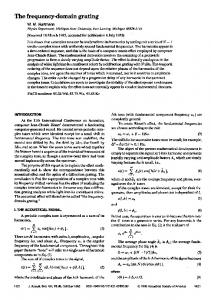
methods to the Fourier transform of the RD functions. The advantages in relation to the usual procedure of spectral density functions estimation, are due to noise reduction from the RD process of averaging time segments of the response, with a common triggering condition, and from avoiding leakage in the spectral densities, as long as the RD functions are evaluated with sufficient time length to have a complete decay within that length. The concepts discussed in this paper will be illustrated in parallel with their presentation, considering the ambient vibration data collected in a ¼ scale model of a 4-story building, which was used in a study conducted at the LNEC triaxial shaking table [7]. The model is presented in figures 1 and 2, as well as some samples of the recorded longitudinal acceleration responses. Just for the sake of simplicity in the exemplification of the concepts, only the longitudinal acceleration records will be considered. 600 kg
600 kg
y4
600 kg
600 kg
y3
600 kg
600 kg
y2
600 kg
600 kg
y1
0.75m
0.75m
0.75m
0.75m
0.10 0.05 0.00 -0.05 -0.10 0.10 0.05 0.00 -0.05 -0.10 0.10 0.05 0.00 -0.05 -0.10 0.10 0.05 0.10 0.00 0.05 -0.05 0.00 -0.05 -0.10 -0.10
y4 (mg)
y3 (mg)
y2 (mg)
y1 (mg)
t (seg.) 0
1.125m
1
2
3
4
5
6
7
8
9
10
11
12
13
14
15
1.125m
Fig. 1 – Dimensions of the model and samples of the acceleration records.
Fig. 2 – View of the model.
The ambient vibration tests of the model presented in figures 1 and 2 were performed with 12 Kinemetrics ES-U force balance accelerometers, signal conditioning equipment constructed at LNEC and data acquisition hardware and software from National Instruments. The equipment was configured for a sensitivity of 4 Volt/mg, and the ambient vibration data was acquired during about 30 minutes using a sampling frequency of 1000 Hz; the records obtained in this way were later pre-processed, with low-pass digital filtering at 25 Hz with a 8 poles Butterworth filter and decimation to a sampling frequency of 62.5 Hz. The results obtained in the example, show that by considering the Fourier transform of the RD functions, a considerable improvement can be achieved, in terms of noise reduction in the spectral density functions with the corresponding quality of the frequency domain output-only modal identification results. 2. Frequency domain output-only modal identification methods There are basically three frequency domain output-only modal identification methods: the basic frequency domain method (BFD) or peak picking method (PP); the frequency domain decomposition method (FDD); and the enhanced frequency domain decomposition method (EFDD). The systematic formulation and implementation of the BFD method can be attributed to Felber [8] although its fundamental ideas had already been used before. Andersen [9] presented some of the basic concepts of the FDD method, but Brincker et al. [1] presented it in a more complete way for output-only modal analysis applications. Brincker et. al. [10] proposed an improvement of the FDD approach, which resulted in the EFDD method. Both FDD and EFDD methods are recently having a widespread use due to their availability in the software Artemis. The common data for the three frequency domain output-only modal identification methods are the estimates of the spectral density functions of the response of a structural system. Usually, those estimates are obtained using a procedure that can be attributed to Welch [11] and consists in: division of the response records in several, eventually overlapped, segments, whose size determines the frequency resolution of the spectral estimates; application of a signal processing window to the data segments in order to reduce the effects of leakage (for
ambient vibration tests signals, the Hanning window is appropriate); computation of the DFT of the windowed data segments trough the use of the FFT algorithm; computation of averaged auto and cross spectra considering the DFT’s of the data segments. Since for identification of the mode shapes of a system, its response has to be measured along several experimental degrees of freedom, one can speak about a matrix of spectral density functions, with auto-spectra in the main diagonal and cross-spectra in the other positions. This matrix can be evaluated completely or a reference-based approach can be adopted, where only the columns (or lines) corresponding to the reference degrees of freedom, are computed. Once the estimates of the spectral density functions are evaluated, the procedures to analyse them, in order to extract the modal properties of a system, are slightly different in each of the methods BFD, FDD and EFDD. In the BFD method the auto-spectra are normalized and averaged in order to obtain an averaged normalized power spectral density function (ANPSD) that, in principle, shows all the resonance peaks corresponding to the vibration modes of a system. Identification of the frequencies of those peaks gives a first idea about the frequencies of the vibration modes of a system. Further analysis is needed of the coherence function and also of the amplitude and phase relations between the records obtained along the different experimental degrees of freedom. Both the coherence function and the amplitude and phase relations are evaluated with the elements of the spectral density functions matrix. At the frequencies of the natural vibration modes of a system, the coherence function should present values close to 1. The amplitude and phase relations between the different degrees of freedom are evaluated with the H1 estimate of the transmissibility frequency response function and can be considered as an estimate of the modal components, from which the mode shapes of a system can be constructed (in fact these are not mode shapes but operational deflection shapes, however the difference between them is insignificant if the system has modes with well separated frequencies and low damping). The BFD method doesn’t have in itself a procedure for estimation of the damping coefficients; however, the halfpower bandwidth method has been widely used in association with it. Another option is to use curve-fitting procedures to adjust SDOF system response auto-spectra to the isolated peaks of the spectral density functions. Especially the first procedure is known to result in rough estimates of the damping. To illustrate the frequency domain output-only modal identification methods, the spectral density functions of the longitudinal accelerations recorded in the tests of the 4-story building model, were evaluated using the above described procedure and considering data segments with 2048 values, which correspond to a frequency resolution of ∆f = 0.031 Hz. Figure 3 shows the ANPSD of the longitudinal accelerations. Table 1 resumes the modal characteristics identified with the BFD method.
Table 1 – Modal characteristics identified with the BFD method. mode f (Hz) floor i 1 2 3 4
1st 2.96
2nd 8.03
3rd 11.69
4th 18.16
Φ1i +0.189 +0.385 +0.811 +1.000
Φ2i +0.662 +1.000 +0.230 -0.708
Φ3i -0.410 -0.351 +1.000 -0.587
Φ4i +1.000 -0.750 +0.149 -0.034
Fig. 3 – ANPSD of the longitudinal accelerations. In the FDD method [1] the spectral density functions matrix is, at each discrete frequency, decomposed in singular values and vectors using the SVD algorithm. By doing so, the spectral densities are decomposed in the contributions of the different modes of a system that, at each frequency, contribute to its response. In each st frequency, the dominant mode shows up at the 1 singular value spectrum and the other modes at the other singular values spectra. From the analysis of the singular values spectra it is therefore possible to identify the auto power spectral density functions corresponding to each mode of a system, which may include parts of several
singular values spectra, depending on which mode is dominant at each frequency. In the FDD method, the mode shapes are estimated as the singular vectors at the peak of each auto power spectral density function corresponding to each mode. The singular values spectra of the longitudinal accelerations are shown in Figure 4. Table 2 resumes the results of the modal identification performed with the FDD method.
Table 2 – Modal characteristics identified with the FDD method. mode f (Hz) floor i 1 2 3 4
1st 2.96
2nd 8.03
3rd 11.69
4th 18.16
Φ1i +0.190 +0.385 +0.811 +1.000
Φ2i +0.662 +1.000 +0.230 -0.708
Φ3i -0.410 -0.352 +1.000 -0.587
Φ4i +1.000 -0.750 +0.150 -0.034
Fig. 4 – Singular values spectra of the longitudinal accelerations. The EFDD method [10] is closely related with the FDD technique, with only some additional procedures to evaluate the damping and to get enhanced estimates of the frequencies and mode shapes of a system. In the EFDD method, the analysis of the singular values spectra, takes a further step forward. The selection of the autospectra corresponding to each mode of a system is performed based on the values of the MAC coefficient between the singular vectors at the resonance peaks and at their neighbouring frequency lines. Those SDOF auto-spectral density functions are then transformed back into the time domain by inverse FFT, resulting in autocorrelation functions for each mode of a system. Enhanced estimates of the frequencies of the modes of a system are obtained from the zero crossing times of those auto-correlation functions (notice that with this procedure the evaluation of the frequencies isn’t restrained to the frequency resolution of the discrete Fourier transform). The damping coefficients are estimated from the logarithmic decrement of those auto-correlation functions. Finally, the estimate of the mode shapes is also enhanced, considering all the singular vectors within each SDOF autospectral density function, weighted with the corresponding singular values. Figure 5 shows the spectrum of the 1st singular value of the spectral density functions of the longitudinal accelerations, with the selected regions corresponding to each mode. Table 3 resumes the results of the modal identification performed with the EFDD method.
Table 3 – Modal characteristics identified with the EFDD method. mode f (Hz) ξ (%) floor i 1 2 3 4
st
nd
rd
th
1 2.98 0.80
2 8.04 0.63
3 11.66 0.73
4 18.18 0.40
Φ1i +0.184 +0.380 +0.812 +1.000
Φ2i +0.659 +1.000 +0.234 -0.708
Φ3i -0.410 -0.372 +1.000 -0.588
Φ4i +1.000 -0.748 +0.145 -0.029
Fig. 5 – Selected spectra for the four vibration modes. For the simple example of the longitudinal modes of the 4-story building model, the results obtained with the three frequency domain output-only modal identification methods, are in good agreement with each other, as it can be seen in tables 1, 2 and 3. It must be mentioned that apart from the peaks corresponding to the longitudinal modes, the spectra shown in figures 3, 4 and 5, also have some smaller peaks, which correspond to torsional
modes of the model, but due to the fact that the model was damaged (it had been used in shaking table tests [7]), those modes are also reflected in the longitudinal accelerations recorded at the geometric centre of each floor. 3. The random decrement technique With the random decrement (RD) technique [2], the structural responses to ambient loads are converted into RD functions. The process of evaluation of the RD functions is a rather simple technique of averaging time segments of the measured structural responses, with a common initial or triggering condition. Initially [1] the RD functions were interpreted as free vibration responses of a system, but latter [12, 13, 5] it has been proved that, under the assumption that the analysed responses are a realization of a zero mean stationary gaussian stochastic process, the RD functions are proportional to the correlation functions of the responses and/or to their first derivatives in relation to time. The interpretation of the RD functions as free vibration responses is almost intuitive, if one thinks that the response of a system to random input loads is, in each time instant t, composed by three parts: the response to an initial displacement; the response to an initial velocity; and the response to the random input loads between the initial state ant the time instant t. By averaging time segments of the response with the same initial condition, the random part of the response will have a tendency to disappear from the average, and what remains is the response of the system to the initial conditions. Since the experimentally measured structural responses always have some noise content, the time segments averaging of the RD technique, also has an effect of reducing the noise in the resulting RD functions. Additionally to auto RD functions, where the triggering condition and the time segments to be averaged are defined in the same response signal, it is also possible to evaluate cross RD functions, where the triggering condition is defined in one response signal and the time segments to be averaged are taken from the other simultaneous response signals. One can therefore evaluate a complete matrix of RD functions, or like in the spectral density functions matrix, a reference-based approach can be adopted, where only a few reference response measurements are considered to apply the triggering conditions. The RD technique is also computationally efficient. For instance, in terms of evaluation of correlation functions, comparisons [12] have been made of different techniques, including the direct method, the FFT based method and the RD technique, showing that the RD technique is faster than the direct method and in many situations faster than the FFT based one (eventually for long estimates of the correlation functions the FFT based method is more competitive [12]). For the evaluation of the RD functions it is possible to consider different triggering conditions [5, 14], namely: level crossing triggering condition; positive points triggering condition; zero crossing with positive slope triggering condition; and local extremum triggering condition. All these can also be interpreted as special cases of a generalized triggering condition [5]. Although there have been some works devoted to spectral estimation [6] and frequency response function estimation [15] using the RD technique, most of its developments [5] have been made in association with time domain modal identification methods, like the Ibrahim time domain method (ITD) [3] or the eigensystem realization algorithm (ERA) [4] which is equivalent to the covariance driven stochastic subspace method (SSI-COV) [16]. This is understandable, since the RD technique is in itself a time domain procedure and therefore it is natural to consider it in association with the time domain identification methods. Using the RD technique, the RD functions were evaluated for the longitudinal accelerations measured in the 4story building model. For that purpose, a level crossing triggering condition was considered, with the optimal value of the triggering level as defined in [5]. In the evaluation of the RD functions, the acceleration records were initially kept at the sampling frequency of 1000 Hz, low-pass filtered at 25 Hz with a 8 poles Butterworth filter, and only the final RD functions were decimated to 62.5 Hz. The RD functions matrix thus obtained is presented in figure 6. The RD functions shown in figure 6 were computed considering time segments with a length of 256 values at 62.5 Hz (about 4 seconds).
Fig. 6 – RD functions matrix of the longitudinal accelerations (length of 256 values). 4. Using the Fourier transform of the RD functions in the frequency domain methods As it has been referred above, the RD functions can be interpreted as free vibrations of a system, therefore a matrix of RD functions, like the one presented in figure 6, can be looked as a set of records from free vibration tests of a system; each column or line of the matrix corresponding to a different test where initial conditions are imposed at the corresponding degree of freedom and the response is measured in all the degrees of freedom. Thus, it seems reasonable to evaluate the spectra of the RD functions, using the FFT algorithm, and to apply the frequency domain output-only modal identification methods to the spectral density functions obtained in such way. It is however necessary to take into account the problems associated with the discrete Fourier transform, namely the effects of leakage. To avoid the effects of leakage, the RD functions must be computed with a total length that allows them to have a complete decay within that length. If this condition is fulfilled then the FFT algorithm can be applied directly to the RD functions, without the need to use signal-processing windows. For the example of the 4-story building model, the RD functions must therefore be computed with a longer length than the one presented in figure 6; it is thus better to use the RD functions presented in figure 7.
Fig. 7 – RD functions matrix of the longitudinal accelerations (length of 2048 values). Notice that the requirement of having RD functions with a complete decay within their length is not an important condition for the time domain methods, but it is an indispensable one for the estimation of the spectral densities as the Fourier transform of the RD functions.
An averaged spectral density functions matrix can be evaluated as the mean of the spectral matrices computed from each column or line of the RD functions matrix. The three frequency domain output-only modal identification methods can then be applied to that averaged spectral density functions matrix, in a similar manner as they are applied to the spectral densities estimated by the more usual Welch’s procedure [11]. The resulting identification methods can be named as RD-BFD, RD-FDD and RD-EFDD since they correspond to a combination of the RD technique with the methods BFD, FDD and EFDD. The advantage in doing this combination is clearly visible in the results that will be presented bellow, and is a consequence of the noise reduction from the averaging of time segments that is performed in the RD technique, and also from avoiding the effects of leakage (if the RD functions are evaluated with enough length to have a complete decay within that length). Figure 8 shows the ANPSD obtained using the RD-BFD method and Table 4 resumes the modal characteristics identified with that method.
Table 4 – Modal characteristics identified with the RD-BFD method. mode f (Hz) floor i 1 2 3 4
st
nd
rd
th
1 2.96
2 8.03
3 11.69
4 18.13
Φ1i +0.187 +0.383 +0.811 +1.000
Φ2i +0.662 +1.000 +0.230 -0.709
Φ3i -0.403 -0.343 +1.000 -0.586
Φ4i +1.000 -0.756 +0.152 -0.037
Fig. 8 – ANPSD of the longitudinal accelerations. Comparing the ANPSD of figure 3 with the ANPSD of figure 8 it is evident that this last one is much more clear; the peaks are quite evident and especially the valleys have a much more rounded shape, showing that the level of noise is very low. There is therefore an advantage in using the RD technique before the estimation of the spectral density functions. The singular values spectra of the longitudinal accelerations, obtained with the RD-FDD method are shown in Figure 4. Table 5 resumes the results of the modal identification performed with that method.
Table 5 – Modal characteristics identified with the RD-FDD method. mode f (Hz) floor i 1 2 3 4
st
nd
rd
th
1 2.96
2 8.03
3 11.69
4 18.13
Φ1i +0.187 +0.383 +0.811 +1.000
Φ2i +0.662 +1.000 +0.230 -0.709
Φ3i -0.404 -0.344 +1.000 -0.586
Φ4i +1.000 -0.756 +0.152 -0.037
Fig. 9 – Singular values spectra of the longitudinal accelerations. If the advantage in using the RD technique was already visible in the ANPSD of the RD-BFD method, then it becomes even more clear in the singular values spectra. Comparing figure 4 with figure 9 it is quite evident that nd rd th while in figure 4 (FDD) there is not much information to be taken from the 2 , 3 and 4 singular values spectra, in figure 9 (RD-FDD) those spectra also have important information about the modal characteristics of the 4-story building model. In fact, the spectra of figure 9 are a good example to illustrate the basic idea of the frequency domain decomposition method – the spectral density functions matrix is decomposed in the contributions of the different modes of a system; those modes appear in the singular values spectra in the order of the weight of their
contribution to the total response. In fact, in figure 9 it is very clear that by joining parts of the singular values spectra, one can form the auto-spectra corresponding to the different modes of the 4-story building model. Figure 10 shows the singular values spectra with the selected regions corresponding to each mode (notice that in this case, much wider regions could have been selected, joining parts of the different singular values spectra, but it was decided to select the same frequency lines that were chosen in the EFDD method). Table 6 resumes the results of the modal identification performed with the RD-EFDD method.
Table 6 – Modal characteristics identified with the RD-EFDD method. mode f (Hz) ξ (%) floor i 1 2 3 4
1st 2.98 0.83
2nd 8.03 0.56
3rd 11.69 0.60
4th 18.17 0.30
Φ1i +0.187 +0.383 +0.811 +1.000
Φ2i +0.662 +1.000 +0.230 -0.709
Φ3i -0.402 -0.339 +1.000 -0.592
Φ4i +1.000 -0.755 +0.153 -0.038
Fig. 10 – Selected spectra for the four vibration modes. The modal characteristics identified with the different frequency domain output-only modal identification methods that were used in this paper, are in good agreement with each other. Actually, the quality of the data measured in the 4-story building model is quite good and therefore the application of the methods BFD, FDD and EFDD with the spectral density functions computed in the usual way, gives already good results. However, by using the spectral densities estimated from the RD functions, the identification of the modal characteristics becomes much more clear (and consequently, also with better results). Figure 11 illustrates the longitudinal mode shapes of the building model with the results identified with the RDEFDD method. The represented shapes where obtained with the aid of a finite element model, by imposing at each floor the experimentally identified modal components. f1 = 2.98 Hz
f2 = 8.03 Hz
f3 = 11.69 Hz
f4 = 18.17 Hz
Fig. 11 – Longitudinal mode shapes identified with the RD-EFDD method. 5. Conclusions The main purpose of this paper was to explore the idea of using the spectral densities estimated from the Fourier transform of the random decrement functions of the response of a system, for the application of frequency domain output-only modal identification methods. To accomplish that intention, the paper presented a brief review of the three main frequency domain output-only modal identification methods, the methods BFD, FDD and EFDD, as well as of the random decrement technique, RD. The explored idea resulted in three methods that were named RD-BFD, RD-FDD and RD-EFDD, since they correspond to a combination of the referred techniques.
The gains of the explored idea in relation to the usual procedure of computing the spectral densities directly from the time series, are due to the noise reduction that results from the time averaging procedure of the random decrement technique, and from avoiding leakage in the spectral densities, as long as the random decrement functions are evaluated with sufficient time length to have a complete decay within that length. The discussed methods were illustrated with the analysis of ambient vibration data measured at a 4-story building model. The results that were presented show that a considerable improvement can be achieved with the explored approach, in terms of reduced noise estimates of the spectral densities, clarity of the modal identification analysis and, consequently, quality of the identified modal parameters. Acknowledgements The contribution of the first author to the work presented in this paper has been developed within the LNEC research project 305/11/14745 on Dynamic Identification of Civil Engineering Structures. References [1] [2] [3] [4] [5] [6] [7] [8] [9] [10] [11] [12] [13] [14] [15] [16]
Brincker, R.; Zhang, L.; Andersen, P. – Modal Identification from Ambient Responses Using Frequency Domain Decomposition, IMAC XVIII, San Antonio, USA, 2000. Cole, H. A. – On-the-line Analysis of Random Vibrations, AIAA Paper No.68-288, 1968. Ibrahim, S. R.; Mikulcik, E. C. – A Method for the Direct Identification of Vibration Parameters from the Free Response, The Shock and Vibration Bulletin, Vol. 47, N. 4, p. 183-198, 1977. Juang, J.-N.; Pappa, R. S. - An Eigensystem Realization Algorithm for Modal Parameter Identification and Model Reduction, AIAA Journal of Guidance, Control and Dynamics, Vol. 8, N. 4, p. 620-627, 1985. Asmussen, J. C. – Modal Analysis Based on the Random Decrement Technique – Application to Civil Engineering Structures, PhD Thesis, Department of Building Technology and Structural Engineering, University of Aalborg, Denmark, 1997. Brincker, R.; Jensen, J. L.; Krenk, S. – Spectral Estimation by the Random Decrement Technique, 9th International Conference on Experimental Mechanics, Copenhagen, Denmark, 1990. Coelho, E.; Campos Costa, A.; Carvalho, E. C.; Ponzo, F. C.; Dolce, M. – Comportamento Sísmico Experimental de Estruturas de Betão Armado Reforçadas com Dispositivos Dissipadores de Energia, REPAR 2000 - Encontro Nacional sobre Conservação e Reabilitação de Estruturas, LNEC, Portugal, 2000. Felber, A. – Development of a Hybrid Bridge Evaluation System, PhD Thesis, University of British Columbia, Vancouver, Canada, 1993. Andersen, P. – Identification of Civil Engineering Structures using Vector ARMA Models, PhD Thesis, Department of Building Technology and Structural Engineering, University of Aalborg, Denmark, 1997. Brincker, R.; Ventura, C.; Andersen, P. – Damping Estimation by Frequency Domain Decomposition, IMAC XIX, Kissimmee, USA, 2001. Welch, P. D. – The Use of the Fast Fourier Transform for the Estimation of Power Spectra, IEEE Transactions on Audio and Electro-Acoustics, Vol. AU-15, N. 2, 1967. Brincker, R.; Krenk, S.; Kirkegaard, P. H.; Rytter, A. – Identification of the Dynamical Properties from Correlation Function Estimates, Bygningsstatiske Meddelelser, Danish Society for Structural Science and Engineering, Vol. 63, N. 1, p. 1-38, 1992. Brincker, R. – Note about the Random Decrement Technique, Aalborg University, 1995. Ibrahim, S. R. – Efficient Random Decrement Computation for Identification of Ambient Responses, IMAC XIX, Kissimmee, USA, 2001. Asmussen, J. C.; Brincker, R. – Estimation of Frequency Response Functions by Random Decrement, IMAC XIV, Dearborn, USA, 1996. Peeters, B. - System Identification and Damage Detection in Civil Engineering, PhD Thesis, Department of Civil Engineering, K. U. Leuven, Belgium, 2000.