improving auditory steadyâstate response

KATHOLIEKE UNIVERSITEIT LEUVEN FACULTEIT INGENIEURSWETENSCHAPPEN DEPARTEMENT ELEKTROTECHNIEK Kasteelpark Arenberg 10, 3001 Leuven (Heverlee) In samenwerking met: FACULTEIT GENEESKUNDE DEPARTEMENT NEUROWETENSCHAPPEN Herestraat 49, 3000 Leuven

IMPROVING AUDITORY STEADY–STATE RESPONSE DETECTION USING MULTICHANNEL EEG SIGNAL PROCESSING

Promoters: Prof. dr. J. Wouters Prof. dr. ir. M. Moonen

Proefschrift voorgedragen tot het behalen van het doctoraat in de ingenieurswetenschappen door Bram VAN DUN

December 2008

KATHOLIEKE UNIVERSITEIT LEUVEN FACULTEIT INGENIEURSWETENSCHAPPEN DEPARTEMENT ELEKTROTECHNIEK Kasteelpark Arenberg 10, 3001 Leuven (Heverlee) In samenwerking met: FACULTEIT GENEESKUNDE DEPARTEMENT NEUROWETENSCHAPPEN Herestraat 49, 3000 Leuven

IMPROVING AUDITORY STEADY–STATE RESPONSE DETECTION USING MULTICHANNEL EEG SIGNAL PROCESSING

Jury: Prof. dr. Prof. dr. Prof. dr. Prof. dr. Prof. dr. Prof. dr. Prof. dr.

ir. Y. Willems, voorzitter J. Wouters, promotor ir. M. Moonen, promotor ir. S. Van Huffel ir. H. Van hamme ir. A.F.M. Snik – Radboud Univ. Nijmegen T.W. Picton – Univ. of Toronto

U.D.C. 534.7

December 2008

Proefschrift voorgedragen tot het behalen van het doctoraat in de ingenieurswetenschappen door Bram VAN DUN

c Katholieke Universiteit Leuven – Faculteit Toegepaste Wetenschappen ° Arenbergkasteel, B-3001 Heverlee (Belgium) Alle rechten voorbehouden. Niets uit deze uitgave mag vermenigvuldigd en/of openbaar gemaakt worden door middel van druk, fotocopie, microfilm, elektronisch of op welke andere wijze ook zonder voorafgaande schriftelijke toestemming van de uitgever. All rights reserved. No part of the publication may be reproduced in any form by print, photoprint, microfilm or any other means without written permission from the publisher. D/2008/7515/120 ISBN 978-94-6018-011-8

Abstract The ability to hear and process sounds is crucial. For adults, the inevitable ongoing aging process reduces the quality of the speech and sounds one perceives. If this effect is allowed to evolve too far, social isolation may occur. For infants, a disability in processing sounds results in an inappropriate development of speech, language, and cognitive abilities. To reduce the handicap of hearing loss in children, it is important to detect the hearing loss early and to provide effective rehabilitation. As a result, hearing of all newborns needs to be screened. If the outcome of the screening does not indicate normal hearing, more detailed hearing assessment is required. However, standard behavioral testing is not possible, so that assessment has to rely on objective physiological techniques that are not influenced by sleep or sedation. The last few decades, the use of auditory steady–state responses (ASSRs) has been investigated as an objective technique to assess hearing thresholds at different frequencies. In this research project, we focus on reducing the required recording time of the ASSR technique and on improving its robustness against unwanted artifacts, generated by e.g. muscle activity, eye blinks, and electrode cable movement. This objective is achieved by processing multichannel electroencephalogram (EEG) recordings. First, we build a setup that allows us to apply custom made stimuli and to record multichannel EEG. Second, the effect of two multichannel processing techniques applied on these data is investigated. Both an independent component analysis (ICA) based technique and a multichannel Wiener filter (MWF) based approach show that a significant measurement time reduction is possible when compared with standard single channel recordings. Afterwards, the ICA– and MWF–based approaches are incorporated into a procedural multichannel framework that is constructed from elements of detection theory. It is shown that this detection theory based approach increases the number of detections significantly when compared with a noise–weighted single channel technique, in the case of artifact–rich EEG. Finally, the optimal electrode positions are determined for the recording of ASSRs originating mainly from the brainstem (and the auditory cortex). After processing with the multichannel EEG processing techniques presented in this work, these positions guarantee a close–to–optimal assessment of the subject’s hearing thresholds. i

ii

Abstract

Korte Inhoud De mogelijkheid om geluiden te horen en te verwerken is cruciaal voor zowel jong als oud. Voor kinderen betekent gehoorverlies een obstakel voor een normale spraak– en taalontwikkeling. Vooral voor hen is het belangrijk om dit gehoorverlies zo vroeg mogelijk op te sporen en er gepast op te reageren. Om deze reden zou het gehoor van alle pasgeborenen moeten worden gecontroleerd. Als het resultaat van deze ‘screening’ niet op een normaal gehoor wijst, is meer gedetailleerde gehoorschatting nodig. Het probleem hier is wel dat de standaard gebruikte gedragstesten niet kunnen gebruikt worden. Om deze reden moeten deze testen terugvallen op objectieve fysiologische technieken die niet be¨ınvloed worden door slaap of sedatie. De laatste decennia werd er gefocust op een techniek die gebruikt maakt van auditieve steady–state responsen (ASSR) om gehoordrempels te schatten op verschillende frequenties. In dit onderzoeksproject proberen we de meettijd te verkorten van de ASSR– techniek en zijn robuustheid te vergroten tegen ongewenste artefacten zoals spieractiviteit. Dit doel wordt bereikt door meerkanaals verwerking van elektroencephalogram (EEG) metingen. Om te beginnen hebben we een opstelling gebouwd waarmee het mogelijk is om zelfgemaakte stimuli aan te bieden aan de proefpersoon en om meerkanaals EEG op te meten. Daarna wordt het effect van twee types meerkanaals signaalverwerking onderzocht die toegepast worden op deze meerkanaals data. Zowel het gebruik van onafhankelijke component analyse (ICA) als een meerkanaals Wiener filter (MWF) maakt het mogelijk om een significante meettijdreductie te bekomen ten opzichte van de standaard éénkanaals metingen. Nadien worden deze ICA– en MWF–gebaseerde benaderingen samengesmolten in een proceduraal meerkanaals raamwerk dat opgebouwd is met bouwstenen uit de detectietheorie. Er wordt aangetoond dat deze benadering het aantal detecties significant vergroot vergeleken met een ruisgewogen éénkanaals techniek wanneer EEG wordt gebruikt dat veel artefacten bevat. Om af te sluiten worden de optimale elektrodeposities bepaald voor het opmeten van ASSR die hoofdzakelijk gegenereerd worden in de hersenstam (en de auditieve cortex). Deze posities garanderen een bijna–optimale schatting van de gehoordrempels van de proefpersoon.

iii

iv

Korte Inhoud

Glossary Mathematical Notation a v M MT M∗ MH = (M∗ )T M−1 X(k : l, :) X(:, k : l) x(i) x(t) X(f ) ˆ ˆ, M a ˆ, v round(x) a=b a∼b a 0.05. Signal–to–noise ratios do not show significant differences using a paired samples t–test for each separate frequency between the two methods, p > 0.05.

3.3.2

Hearing threshold difference scores

Table 3.1 presents the mean differences between the measured ASSR thresholds and the corresponding behavioral thresholds. A paired samples t–test does not show any significant differences for each separate frequency between the two methods, p > 0.05.

58

SOMA: A Research Platform for Multichannel ASSR Measurements 35

Response 30

Amplitude (nV)

25 20 15

Noise

10 5 0 0.5

1 2 Frequency (kHz)

4

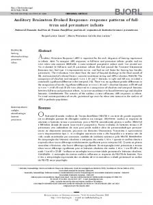
Figure 3.8: Mean ASSR and noise amplitudes (nV) for 40 dBSPL data of nine subjects for measurements of 32 sweeps. MASTER: solid line & square marker. SOMA: dotted line & circle marker. The noise amplitude per frequency is estimated around its corresponding modulation frequency using the RMS value of N = 120 neighboring frequency bins, approximately 3.7 Hz (60 bins) at each side. Response and noise values of the same carrier frequency (left and right) are taken together for analysis, e.g. 1 kHz in the figure shows both response and noise values of modulation frequencies 90 and 94 Hz. Error bars are omitted for clarity. Standard deviations (nV) are 11.9, 16.5, 16.1, 8.7 and 8.9, 11.9, 14.3, 9.1 for MASTER and SOMA response amplitudes respectively. For noise amplitudes the standard deviations (nV) are 2.5, 2.6, 2.6, 2.6 and 2.5, 2.6, 2.7, 2.9 for MASTER and SOMA respectively.

3.4

Discussion

This chapter focusses on the development of a setup for multichannel auditory steady–state response measurements, called SOMA – Setup ORL for Multichannel ASSR. Both the hardware and software implementation are described, together with an evaluation study on nine normal–hearing subjects. The urge for the development of an alternative research setup, next to the currently available commercial devices, was created by the need for a mobile, multichannel, inexpensive, flexible and modular extensible research platform, capable of processing custom made stimuli and changing carrier frequency intensities on the fly. Most commercial devices do not provide more than two–

3.4. Discussion

59

channel EEG measurements. The possibility to read in own stimuli or to alter stimulus and recording parameters is very limited or non–existent. Adding extra functionalities without referring to the manufacturer is not possible. If research is the main purpose, commercial devices often do not fulfill the researcher’s expectations although these devices are highly suitable in their respect for use in clinical environments. SOMA uses a standard high–quality multichannel RME soundcard. This soundcard based choice is motivated by the fact that the RME soundcard is relatively inexpensive compared to standard multichannel data acquisition cards, by the use of several RME devices in the author’s research environment, the available experience built up through this presence and the availability of C++ software code for the device. A portable SOMA prototype setup using a RME soundcard was built up in a very short time in combination with multichannel recording software, like e.g. Adobe Audition. The prototype showed that stimulus presentation over a wide dynamic range needed for ASSR measurements was possible using the RME soundcard and that is was capable of recording multichannel amplified EEG potentials. The sufficient dynamic range makes it possible to avoid the use of attenuators or audiometers which keeps the setup portable. The most important advantages of the setup are the use of multiple EEG channels, the use of custom stimuli and the flexibility for research studies. Two–channel measurements are available in the most recent ASSR devices of e.g. Natus, Interacoustics, Grason–Stadler Inc. or Intelligent Hearing Systems. The use of more than two channels however, is not available commercially. Some devices are more flexible than others, but in general the possibilities to change experiment stimuli or parameters is limited. Minor advantages are the portability, the possibility to change independent intensities on the fly (also implemented by Interacoustics) and the modular extensibility, which makes the user independent from a commercial supplier. The biggest limitation of the SOMA setup is the intensity range of 10 to 100 dBSPL (90 dB dynamic range). This seems rather low compared to other devices, but it is considered sufficient for hearing threshold determination for both normal–hearing as severely hearing impaired subjects. Table 3.1 can be compared to studies with other multiple frequency ASSR thresholds in normal hearing subjects (Dimitrijevic et al., 2002; Herdman and Stapells, 2001; Luts and Wouters, 2005; Perez-Abalo et al., 2001), that use the same MASTER–system as in this study, except for Perez-Abalo et al. (2001) who use the Audix system from Neuronic S.A. Standard deviations of the difference scores are comparable to the current data. The difference scores are lower than those achieved by MASTER and SOMA in the present study, except for the data in Luts and Wouters (2005), which are similar. Reasons for the lower difference scores in the other three studies can be found in elevated hearing thresholds or longer test durations (Luts and Wouters, 2005).

60

SOMA: A Research Platform for Multichannel ASSR Measurements

Table 3.1: Mean difference scores and standard deviations of the ASSR threshold (measured at 10 dB precision) and the corresponding behavioral threshold (measured at 5 dB precision) for 18 normal–hearing ears. Intensities of 50, 40, 30, 20 and 10 dBSPL have been applied in experiments of 32 sweeps each (approximately 10 minutes). In some cases, a 60 dBSPL intensity has been used to confirm a threshold. Carrier (Hz) MASTER (dB) SOMA (dB)

3.5

500 22 ± 11 24 ± 9

1000 15 ± 8 19 ± 9

2000 14 ± 7 15 ± 8

4000 17 ± 8 16 ± 9

All 17 ± 9 18 ± 9

Conclusions

Section 3.1 describes the general background and the motivation for building the setup. Commercially available setups do not provide the specifications required for the studies in this thesis. Therefore it is decided to build a custom setup. In Section 3.2, both hardware and software of the setup are described. SOMA makes use of an inexpensive multichannel soundcard that is controlled by software written in C++. Section 3.3 presents the results of an evaluation study with nine normal–hearing subjects that shows that no significant performance differences exist between the proposed platform and a reference platform (the MASTER platform from John and Picton (2000a)). These observations are discussed in Section 3.4. It can be concluded that the SOMA program, in combination with the RME multichannel soundcard, can be used to assess ASSR hearing thresholds reliably. SOMA presents a flexible and modularly extensible high–end mobile ASSR test platform, that allows multichannel measurements, the use of own stimuli and independent intensity changes. It is not restricted by the limitations of commercial software and is thus suited for research and several clinically diagnostic purposes. Although the validation study was conducted using only single channel measurements, an extension to multiple channels will not compromise these conclusions. In the following chapters the SOMA setup is used to apply generated and custom made stimuli and to record multichannel EEG. This multichannel EEG is processed using different multichannel signal processing techniques.

Chapter 4

Improving ASSR Detection Using Independent Component Analysis Section 2.1 showed that auditory steady–state responses are a reliable assessment technique for hearing threshold estimation. Unfortunately, ASSR measurements can last a long time. To reduce recording time to about 45 to 60 minutes, Section 2.2 offered several solutions. Although being effective in most of the cases, these methods were not developed with multichannel EEG measurements in mind. The following chapters will address the processing of multichannel EEG data. This way, measurement times can be reduced significantly and robustness against artifacts can be increased. The first multichannel processing technique discussed in this thesis is independent component analysis (ICA). After a short introduction in Section 4.1, Section 4.2 introduces the theory of ICA, its assumed ASSR model, the experimental setup and the used evaluation method. In Section 4.3, the theory is applied to real–life EEG data. Firstly, the available seven–channel data of eight normal–hearing subjects are processed based on ICA (using the JADE algorithm) and results are compared to those from the most common single channel ASSR technique (John and Picton, 2000a). It will be shown that ICA significantly improves detection for measurements between 30 and 60 dBSPL. Secondly, the optimal number of input channels, the optimal electrode positions The material presented in this chapter has been published in ‘Van Dun, B., Wouters, J., and Moonen, M. (2007), “Improving auditory steady–state response detection using independent component analysis on multi–channel EEG data,”IEEE Trans. Biomed. Eng., 54(7), 1220–1230’.

61

62

Improving ASSR Detection Using ICA

and the optimal number of independent components are reported. Thirdly, by fixing the separating matrix W, calculated from data with a high SNR, a performance improvement may be expected. This assumption is evaluated. Fourthly, the performance of an ICA–based procedure applied to single channel data is considered. Finally, a combination of previous techniques is presented. Section 4.4 discusses these results. Section 4.5 ends this chapter with some conclusions.

4.1

Introduction

Over the last decade, independent component analysis (Hyvärinen et al., 2001) has appeared as a powerful signal analysis tool for a variety of industrial, medical and even financial applications (Back and Weigend, 1997; Bounkong et al., 2003; De Lathauwer et al., 2000; Fang and De-Shuang, 2005). ICA allows finding the underlying factors from multivariate statistical data by looking for components that are both statistically independent, and non–Gaussian. In this chapter, the possible use of ICA in ASSR detection is investigated.

4.2

Methods

This section describes the methods used in this study. In Section 4.2.1, the theory of independent component analysis is presented. When ICA is applied to the recorded multichannel EEG containing ASSRs, a model needs to be assumed (Section 4.2.2). Sections 4.2.3 and 4.2.4 describe the used setup and stimuli for the evaluation study. The single channel reference method and the way the multichannel EEG is processed using ICA is described in Section 4.2.5. Finally, the used performance evaluation procedure is described in Section 4.2.6.

4.2.1

Independent component analysis

Independent component analysis (ICA) is a blind source separation technique that is used to find a latent structure underneath a set of observations (Comon, 1994; Hyvärinen et al., 2001). This underlying structure comes in the form of unknown sources or independent components (ICs). The ICA general model is X = f (θ, S)

(4.1)

with XT = [x1 x2 . . . xm ] a matrix with m observations xi and f an unknown function with parameters θ that operates on statistically independent underlying variables ST = [s1 s2 . . . sq ] with q ≤ m. If f is a linear function, a special

4.2. Methods

63

case of the above equation is obtained, namely X = AS

(4.2)

with A an m × q mixing matrix. The pseudoinverse of A is defined as the separating matrix W, W = A+ (4.3) This formula states that each of the observations xi is a linear combination of a set of q underlying ICs sj : xi = ai1 s1 + . . . + aiq sq

for i = 1 . . . m

(4.4)

ICA–algorithms estimate both S and A. The most important assumption of ICA is that the components, linearly combining into observations, are mutually independent of each other. The fundamental problem is how to assess the independence of the components. The more common approach assumes the distributions of the ICs to be as far from normal Gaussian as possible. This idea is fed by the inverse of the central limit theorem, which states that the distribution of a sum of independent variables shifts to a normal (Gaussian) distribution when the number of variables goes to infinity (Trotter, 1959). To make this approach practically usable, different approximate measures of non–Gaussianity have been developed. By maximizing such a measure, a matrix S can be constructed numerically. The ICA–algorithm that has been used in the rest of this study is the joint approximate diagonalization of eigenmatrices (JADE) algorithm (Cardoso and Soloumiac, 1993). This algorithm has advantages over e.g. FastICA (Hyvärinen, 1999) that practically suffers much more from local optima, leading to the calculation of different ICs and separating matrices W when the algorithm is run several times over the same dataset. However, alternative algorithms could have returned a higher performance than JADE, like the recent MILCA algorithm (Stögbauer et al., 2004). It is possible to tailor the ICA–algorithm to specific needs of the problem using the Bayes theorem (Knuth, 1999). An extension of ICA to underdetermined mixtures is also a possible approach (Comon, 2004; Deville et al., 2004). At the time of this research, JADE was considered a proven technique that was tested on several applications, while the new methods above did not have those benefits that much.

4.2.2

Assumed model

In Section 4.2.3, a seven–channel setup will be described that records linear combinations of an unknown number Q of latent sources. When eight ASSRs are present one can assume eight latent sources to be ASSRs, as these sources are assumed to be independent from each other. This assumption is not correct anatomically when intensity, number of responses, carrier– and modulation frequency are varied (Lins and Picton, 1995). However, when all these parameters

64


are kept fixed, the assumption holds as each modulation frequency excites a different part of the brainstem (Picton et al., 2003). This assumption is also supported by our own experience that ICA–application on real EEG data shows that not all ASSRs are projected on one single independent component. It is assumed in this model that each ASSR is generated by only one source. If not, the number of ASSR sources will be larger than eight. This however does not impact on the model and conclusions. Condensing this in a generative model, one obtains X = BS + N:  

  x1  ..    . = x7

b11 .. .

b12 .. .

b71

b72

... .. . ...

b1Q .. . b7Q

sASSR1 sASSR2 .. .

     sASSR7    sASSR8   snoise1   ..  . snoiseQ−8

         +      

 n1 ..  .  n7

(4.5)

where sASSRi (i = 1, . . . , 8) are ASSR sources, snoisej (j = 1, . . . , Q − 8) are muscle artifacts, eye blinks, brain processes, . . . and nk (k = 1, . . . , 7) are external noise sources like amplifier noise and e.g. line noise picked up by the electrode cables. When observing (4.5), each row k in B gives information about the SNR of a certain ASSR in the corresponding observation xk . Therefore, it is possible to look for the xk with the highest SNR for each ASSR source. After application of ˆ = WX), B is replaced by B ˆ = WB. The simulations from Section 4.3 ICA (S ˆ are expected to show that B returns a better SNR for an ASSR in certain ˆ than B for an ASSR in the observation matrix X. It components from S ˆ this way that will is likely that the ICA–technique can assess components S be more useful for detection than the original observations X, based on the assumption that ASSR sources have a platykurtic distribution, while the EEG noise sources have a more mesokurtic one (close to Gaussian).

4.2.3

Experimental setup

The ASSR measurements were conducted in a sound–proof Faraday cage. The recording electrode placement can be found in Table 4.1, in accordance with the international 10–20 system of Figure 2.2 (Malmivuo and Plonsey, 1995). All seven active electrodes were referenced to the common electrode, which was placed on the forehead. The Kendall electrodes were placed on the subject’s scalp after the skin was abraded with Nuprep abrasive skin prepping

4.2. Methods

65

Table 4.1: Recording electrode positions for a seven–channel setup. All channels are referenced to the common electrode on the forehead. The configuration for the single channel reference method is denoted using bold typeface. Channel 1 2 3 4 5 6 7 common ground

Position Oz P4 P3 Cz F4 F3 Pz forehead left mastoid

gel. A conductive paste was used to keep the electrodes in place and to avoid that inter–electrode impedances exceeded 5 kΩ at 30 Hz. The electrodes were connected to a low–noise Jaeger–Toennies multichannel amplifier. Each EEG channel was amplified (× 10,000), bandpass filtered between 70 and 120 Hz (6 dB/octave) and finally software highpass filtered at 75 Hz (60 dB/octave). The amplified EEG signals were read using an RME Hammerfall DSP Multiface multichannel sound card and recorded using Adobe Audition 1.0 at a sampling rate of 32 kHz and downsampled to 250 Hz. Downsampling does not influence the performance of the ICA–algorithm, but greatly improves its efficiency. An alternative for downsampling could exist in the use of these extra samples to create additional artificial channels. All offline processing was performed using Matlab R14. The sound card was also used to generate the stimuli (see below). In the end, the stimulation and recording equipment used here is an older version of, but very similar to, the setup described in Chapter 3. An artifact rejection protocol was used, where all epochs (data blocks of 256 samples) greater than 20 µV in absolute value were rejected. Eight normal–hearing volunteers (age range 22–33 years) participated in the study. Their behavioral hearing thresholds were less than 20 dBSPL for octave audiometric frequencies between 500 and 4000 Hz. Subjects were asked to lie down on a bed with eyes closed and to relax or sleep. Four trials with a length of 48 sweeps each (approximately 13 minutes) were conducted: at 60, 50, 40 and 30 dBSPL respectively. These intensities were chosen as the main goal of the study was to decrease the measurement duration, and not hearing threshold assessment in general. At the end of the session, behavioral thresholds were determined at 0.5, 1, 2 and 4 kHz with a 5 up–10 down method using modulated sinusoids.

66

4.2.4


Stimuli

Two stimuli with four 100% amplitude modulated (AM) carrier frequencies each, were applied to each ear. The carrier frequencies were the same for both ears, namely 0.5, 1, 2 and 4 kHz. The modulation frequencies were taken close to respectively 82, 90, 98 and 106 Hz for the left ear, and 86, 94, 102 and 110 Hz for the right ear. To obtain an integer number of modulation frequency cycles in one data block of 256 samples (1.024 seconds), the previous values had to be corrected slightly (John and Picton, 2000a). This stimulus configuration was used with four out of eight subjects. The other four subjects received a reduced stimulus set, with only 0.5 & 4 kHz applied to the left ear and 1 & 2 kHz to the right ear. This difference in stimulus sets does not influence the following results. Stimuli were created using Matlab R14 and played using Adobe Audition 1.0 at a sampling rate of 32 kHz. An RME Hammerfall DSP Multiface multichannel sound card sent the stimuli to Etymotic Research ER–3A insert phones for subject stimulation. The eight separate signals were calibrated at 70 dBSPL, using a Br¨ uel & Kjær Sound Level Meter 2260 in combination with a 2–cc coupler DB138.

4.2.5

Five ways to process the available EEG dataset

This subsection describes five different ways to process the available multichannel EEG. These methods are all evaluated in this chapter. The first method serves as the (standard) reference method all other methods are compared with. The third method is a combination of the first and the second method. The fifth method is a combination of methods 1, 2 and 4. It will be shown that these combinations of methods will increase performance compared with the individual methods. Method 1: Single channel reference method All ICA–processed EEG data in this chapter is compared with a gold standard, a single channel reference method that is most commonly used in clinical practice and described in literature (for an extensive review of single channel recording techniques, we refer to Picton et al. (2003)). For adults this single channel reference technique is the placement of the active and reference electrodes at Cz (inion) on top of the head and Oz (occiput) at the back of the head just above the base of the skull. The ground electrode position is not relevant. According to Table 4.1, channel 1 (Oz) and channel 4 (Cz) are both referenced to the common electrode at the forehead. When channel 1 (Oz–forehead) is subtracted from channel 4 (Cz–forehead), a new EEG channel is obtained

4.2. Methods

67

between electrodes Cz and Oz. This new channel is defined as the reference channel for single channel measurements. The EEG data in channels 1 and 4 were artifact rejected (20 µV ) according to Section 4.2.3 before taking the difference of both channels. Enough data was collected such that the data stream could be divided into N = 48 sweeps. One sweep is exactly 16.384 seconds long (or M = 4096 samples), based on parameters also used in John and Picton (2000a). Initial recording lengths were such that the division in 48 sweeps was always possible after artifact rejection. This implies that measurements with subjects generating a lot of artifacts are longer compared with measurements with subjects that do not produce that many artifacts. Data is averaged over N sweeps with equal weights (normal averaging) according to the steps below. • The single channel EEG recordings are divided in 48 data blocks (sweeps) with a length of 4096 samples (16.384 seconds). • Each sweep sn (n = 1 . . . 48) is averaged together with all preceding sweeps s1 to sn−1 . This creates 48 averaged sweeps s¯n (n = 1 . . . 48) with a length of 4096 samples. Averaged sweep s¯1 is identical to sweep s1 . Averaged sweep s¯48 is an average of all sweeps s1 to s48 . This averaging step is necessary to increase the SNR of the ASSR to an acceptable level. • For each processed (averaged) sweep s¯n , the F–ratio (SNR) of each modulation frequency is determined using (2.11). When 8 modulation frequencies are used, 8 F–ratios are calculated. All ICA–processed results in this chapter (and the results obtained after MWF– processing in Chapter 5) are compared with this reference method. Method 2: Multichannel ICA The sketchy algorithm below processes m–channel EEG data with a length of N M samples. N is the number of sweeps (data blocks) the data will be divided into. In this chapter the data is divided into N = 48 sweeps. One sweep is 16.384 seconds long (or M = 4096 samples), based on parameters also used in John and Picton (2000a). This m × N M EEG data matrix is, after artifact rejection and an averaging step, processed using the ICA–technique from Section 4.2.1 to obtain q independent components (ICs). For clarity, the description will explicitly show the process using N = 48 sweeps and M = 4096 samples. The number of channels m and the number of ICs q are kept variable. • The m–channel EEG recordings are divided in 48 m–channel data blocks (sweeps) with a length of 4096 samples (16.384 seconds).

68

Improving ASSR Detection Using ICA • Each m–channel sweep sn (n = 1 . . . 48) is averaged together with all preceding sweeps s1 to sn−1 . This creates 48 averaged m–channel sweeps s¯n (n = 1 . . . 48) with a length of 4096 samples. Averaged sweep s¯1 is identical to sweep s1 . Averaged sweep s¯48 is an average of all sweeps s1 to s48 . This averaging step is necessary to increase the SNR of the ASSR to an acceptable level. Without averaging, the ICA–technique will fail, in contrast with the MWF–method from Chapter 5 that actually does not need prior averaging. • The JADE algorithm takes one averaged m–channel sweep s¯n as an input. • q ICs are calculated based on the m–channel averaged sweep s¯n (with a length of 4096 samples). Each IC also has a length of 4096 samples. • For each IC in a processed (averaged) sweep, the F–ratio (SNR) of each modulation frequency is determined using (2.11). When 8 modulation frequencies are used, 8 F–ratios are calculated. Consequently, when q ICs are available, 8q F–ratios are calculated for each processed (averaged) sweep s¯n . • For each modulation frequency within the same processed (averaged) sweep s¯n , the largest F–ratio is taken out of q calculated F–ratios.

This procedure is not used directly in this chapter, but is improved first as described by method 3. Method 3: Multichannel ICA combined with single channel reference method (method 1 + 2) The first simulations using method 2 show a major variation over the different subjects, with several subjects performing worse than the single channel reference (method 1). The general improvement is marginal. To avoid this effect, methods 1 and 2 are combined. In particular, the best F–ratio out of q + 1 F–ratios for each modulation frequency is taken: q F–ratios from the q ICs calculated using method 2 with m EEG–channels as an input and one extra F–ratio from the original single channel reference using method 1. One should be aware that this combination of both the single– and multichannel approach does not necessarily ensure a better performance, compared to the single channel reference using method 1. As it is important to keep the specificity of the combined processing (method 3) equal to the specificity of the reference (method 1), the single channel data should truly be viewed as an extra channel, which raises the detection threshold accordingly due to the multiple testing aspect (Section 4.3.1). The results obtained by applying this procedure on multichannel EEG data is described in Sections 4.3.1, 4.3.2 and 4.3.3.

4.2. Methods

69

Method 4: Single channel ICA combined with single channel reference (method 1) Some research already has been conducted on the single channel case of independent component analysis (Davies and James, 2007; James and Lowe, 2003; Warner and Proudler, 2003). Single channel ICA contradicts the intuition that ICA is only suitable for processing of multichannel measurements. Recently, it has been suggested by Davies and James (2007) that single channel ICA (SCICA) can identify and separate sources successfully only when these sources have disjoint spectral support. However, if one–channel data is divided in different channels (say, two), it may still be worth the effort to check whether the algorithm may be able to extract two components with the following characteristics. The first component may be the ASSR of interest, which is presumed to be present in both (divided) channels, in the form of a sinusoid at a certain frequency. The second component may be the background EEG noise. One may argue that the non–stationary EEG noise varies too much over the two created channels. However, the chance that the statistical properties of the EEG noise from the first channel are totally different from those of the EEG noise of the second channel, is considered low. A limitation of the ICA–technique is that the number of q ICs cannot exceed the number of m observations or channels. Otherwise the ICs are not identifiable because A is not invertible. Therefore, no more than one IC can be estimated from single channel data, and then – quite trivially – this IC would be equal to the original data. To avoid this problem, the available data has to be split up to create m − 1 extra artificial channels, so that m channels are available to calculate q ICs. Other approaches may also be used to create extra channels. First, when the available single channel EEG data is oversampled, extra channels can be created by downsampling the data multiple times, with a shift by an integer number of samples for each new downsampling step. Second, an interesting procedure is described in Davies and James (2007). Extra channels are created by shifting the available single EEG channel a couple of times by one sample each (thus creating a Toeplitz matrix with ‘EEG channels’). After application of a multichannel ICA–algorithm, the ICs are clustered with a clustering algorithm. Based on the acquired clusters, reconstruction filters are calculated that can be applied on the original single channel EEG data. A schematic overview is shown in Figure 4.1 of the used single channel ICA– technique applied to a one–channel EEG data stream with a length of N M samples. This EEG data stream is the same (reference) channel (Cz–Oz) as used in method 1. N is the number of sweeps (data blocks) the data will be divided into, after artefact rejection (20 µV ). In this chapter the data is divided into N = 48 sweeps. One sweep is 16.384 seconds long (or M = 4096 samples), based on parameters also used in John and Picton (2000a). For the sake of simplicity, the description will explicitly show the process using N = 48 sweeps and M = 4096 samples per sweep. The number of channels m and

70


ICs q is taken equal to 2. This has been observed to be the optimal number of channels and ICs for the single channel case (Section 4.3.4). Other values for m and q degrade performance significantly. The single channel procedure is as follows: • Step 1) An 48×4096 matrix is constructed from the data stream originating from the single channel recording system described in Section 4.2.3. No averaging has been carried out yet. This matrix is divided in m = 2 parts (‘channels’ or ‘observations’), by interleaving the odd and even N sweeps, with m = 24 sweeps per part, each sweep 4096 samples long. Part 1 contains sweeps s1 , s3 , . . . , s47 and Part 2 contains all even– numbered sweeps. • Step 2) Sweeps s1 , s3 , . . . , s2k−1 from Part 1 are averaged and stored in sweep sk of an averaged matrix (k = 1, . . . , 24). Sweeps s2 , s4 , . . . , s2k from Part 2 are averaged and stored in sweep s24+k of that averaged matrix (k = 1, . . . , 24). The resulting averaged matrix has the same structure as the matrix from Step 1. • Step 3) Independent component analysis is performed 24 times, each time using a group of m = 2 sweeps sk and s24+k from the matrix from Step 2 with k = 1, . . . , 24. Each element from this group of sweeps shares the property that the element is constructed by averaging k sweeps from the matrix from Step 1. For each k, the JADE algorithm takes in m = 2 observations and returns q = 2 ICs, which are linear combinations of sweeps sk and s24+k . • Step 4) For each k, every IC from Step 3 is Fourier transformed and the F–ratio (SNR) is calculated of the modulation frequency of interest using (2.11). Because ICA does not order its components in any way (rows in A can be permuted randomly), it is unknown which component has the highest F–ratio of a certain modulation frequency. For each modulation frequency, all F–ratios (SNR) from all q = 2 ICs are calculated and the largest one is chosen. • Step 5) After the largest F–ratio is chosen, a dimension problem arises. If only one F–ratio is calculated out of m = 2 sweeps from an N = 48–sweep N data stream, only m = 24 F–ratios are available. To compensate for this, each IC has to be copied 2 times to make comparison possible with the single channel reference from method 1, which still contains 48 sweeps after averaging. As such, the resulting sweep from an ICA–operation on 2 sweeps replaces those 2 sweeps by the resulting sweep and its copy. The first simulations using single channel ICA only show no performance increase. However, when the single channel ICA–approach is combined with

4.2. Methods

71

FFT

F-RATIO

FFT

F-RATIO

MAX F-RATIO

F-RATIO FOR 2 CONSECUTIVE SWEEPS

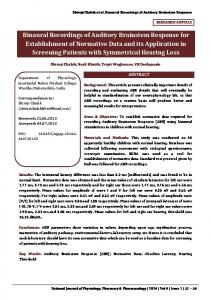
Figure 4.1: Data flow for ICA applied on single channel data. Artificial input channels are created by splitting the available data in m = 2 different parts. These parts are used to calculate q = 2 independent components. method 1, there is some improvement (we refer to Section 4.3.4 for the results). In particular, the best F–ratio out of 3 F–ratios for each modulation frequency is taken: 2 F–ratios from the 2 ICs calculated using the method described in this subsection with the single channel reference (Cz–Oz) as an input and one extra F–ratio from the original single channel reference (Cz–Oz) using method 1. The results obtained after application of this procedure are described in Section 4.3.4.

Method 5: Multichannel ICA combined with single channel reference method and single channel ICA (method 1 + 2 + 4) The procedures from method 3 (which itself is a combination of methods 1 and 2, results described in Sections 4.3.1, 4.3.2 and 4.3.3) and method 4 (results in Section 4.3.4) are combined. The best F–ratio out of q + 3 F–ratios for each modulation frequency is taken: q F–ratios from the q ICs calculated using method 2, one F–ratio from the original single channel reference using method 1, and two F–ratios obtained with method 4 (here, 2 ICs are extracted from single channel EEG data). The results obtained by applying this procedure on multichannel EEG data is described in Section 4.3.5.

72


4.2.6

Performance measures

For evaluation of the proposed techniques, two methods have been chosen. The first one uses receiver operating characteristic (ROC) curves. It has the possibility to indicate statistically significant differences between techniques. However, ROC–curves do not give insight in the absolute benefit from one method compared to another one in terms of measurement time. Therefore, a second measure represents the amount of time that is needed to obtain a significant response. The drawback here is that the results do not have a statistical meaning and only give an indication for what is possible for an individual subject.

ROC–curves In order to evaluate the above described techniques, receiver operating characteristic (ROC) curves were calculated from 8 subjects (Green and Swets, 1966; Hanley and McNeil, 1982). The curves were constructed as follows for a certain number of averaged sweeps: 1. Select 50 decision criteria pi , represented by p–values that vary between 0.9 and 10−15 . TP 2. For each decision criterium pi , calculate the sensitivity TP+FN and speciTN ficity FP+TN over all measurements (4 intensities per subject), using 16 modulation frequencies of which 8 were used as control frequencies, as in these frequencies it was assured that only noise was present. A true–positive (TP) is a correct assessment from the algorithm that a response is present in reality. A false–negative (FN) is an uncorrect assessment that no response is present, while in reality a response is there. True–negatives (TN) and false–positives (FP) are the dual cases. All TP, TN, FP and FN are summed together over the same decision criterium pi and used in the above equations.

3. The ROC–curve is built up plotting the ‘sensitivity’ as a function of ‘1specificity’. Each pi defines a new point of the curve. After plotting all 50 points of the ROC–curve, the area below the curve is calculated. The area under the curve was used as a measure of detection accuracy. This procedure is carried out for each evaluated method. These calculations were carried out each time an additional sweep was collected and averaged with previous sweeps, so that the performance could also be analyzed on a time based scale.

4.2. Methods

73

To statistically compare different ROC–areas, a Z–test was carried out. The z–value can be calculated using (Hanley and McNeil, 1983): z=p

A1 − A2 σ12 + σ22 − 2rσ1 σ2

(4.6)

with A1 the ROC–area calculated for method 1 (the single channel reference) and A2 the ROC–area calculated for all other methods (single– or multichannel ICA). Here, σi is the standard deviation of Ai and r is the correlation coefficient between the data obtained from method 1 and the other methods. The σi are calculated using r X1 + X2 + X3 σi = (4.7) nA nN with

X1 X2 X3 nN nA Q1

= Ai (1 − Ai ) = (nA − 1)(Q1 − A2i ) = (nN − 1)(Q2 − A2i ) = TP + FN = TN + FP Ai = 2−A i

Q2

=

2A2i 1+Ai

where nA are all ‘abnormal’ (negative in reality) cases and nN all ‘normal’ (positive in reality) cases. To find r, a value must be looked up in Table I of (Hanley and McNeil, 1983) using rN , rA , A1 and A2 . Here, rN is the Pearson Product–moment correlation between all processed normal data (nN ) from method 1 and the other methods. In the same way rA is calculated with all abnormal data (nA ). As an alternative, r can be taken as the mean of rA and rN which produces a maximum error on r of 10 %.

Effective measurement time reduction ROC–curves provide a theoretical means to assess different methods. To evaluate the practical applicability of a method, a measure for the effective benefit can be obtained by counting the number of processed sweeps until a response is first–detected. The difference between these numbers obtained with the two methods is an indication for a practical improvement or decline. In this study, we define a first–detection to be valid when the response is significantly present for 3 consecutive sweeps for methods 3 and 4, and 6 consecutive sweeps for method 5. In Chapter 5, this evaluation method is also used for an MWF– based approach. Here, 8 consecutive sweeps are required for detection. This quantity is based on the condition that there is no improvement allowed for noise frequencies when comparing methods 3, 4, 5 and the MWF–based approach from Chapter 5, with the single channel reference (method 1).

74


Due to the statistical multiple testing effect, the detection threshold (a p–value which is calculated by applying an F–test as described in Section 2.2.6 on the finally selected (maximum) F–ratio) needs to be made more stringent when adding more ICs for detection. The p–values for detection are the following: p = 0.050 (method 1), p = 0.0065 (method 3), p = 0.020 (method 4), p = 0.0053 (method 5), and p = 0.00025 (MWF–based approach of Chapter 5). One needs to keep in mind this evaluation method is patient dependent and relies much on the used detection criterion.

4.3

Results

This section presents the results when applying ICA to the recorded single– and multichannel EEG. Section 4.3.1 will show the effect of extracting seven independent components out of seven EEG channels. Section 4.3.2 describes what happens when the number of EEG channels and the number of independent components are varied. Section 4.3.3 introduces the fixed separation matrix. These sections describe the results obtained using implementations of method 3, with method 1 used for comparison purposes. Section 4.3.4 shows ICA applied to only one EEG channel, an application of method 4. Finally, multichannel and single channel ICA are combined using method 5 in Section 4.3.5. Figures 4.2, 4.4, 4.5, 4.6 and 4.7 show the area under the ROC–curve as a function of the number of averaged sweeps for different methods, compared with the single channel reference (method 1). The reference method is the standard single channel MASTER setup (John and Picton, 2000a) with artifact rejection at 20µV and with the amplified difference between Cz and Oz as EEG signal. This setup is described in more detail in the first part of Section 4.2.5. A paired Z–test was carried out (Section 4.2.6) to compare the different techniques statistically using ROC–curves. The dotted lines in Figures 4.2, 4.6 and 4.7 denote two standard deviations of the ROC–areas. When they do not overlap, a significant difference is present (94.7 % significance interval, two standard deviations). Important for clinical application is the fact that, with the current sampling rate of 250 Hz, a real–time calculation during measurement is possible. Every 16.384 seconds, a new sweep is read. On a high–end PC (Pentium 4), the calculation time of the seven–channel ICA does not exceed five seconds. As a result, each new sweep can be downsampled, processed online and visualized before the next one is collected.

75

Area under ROC Curve

4.3. Results

Number of Averaged Sweeps

Figure 4.2: ‘area under ROC–curve’ versus ‘number of averaged sweeps’: Method 3 with q = 7 independent components and m = 7 channels (dashed); Method 1, single channel reference (solid). The dotted lines denote two standard deviations.

4.3.1

Multichannel ICA (method 3): seven channels and seven extracted components

ROC Figure 4.2 shows the results of method 3 with q = 7 independent components and m = 7 channels. A significant difference (two standard deviations) between the single channel reference (method 1) and multichannel ICA–configuration (method 3) is present from sweep 11 on. The best performance of the single channel reference (method 1) is obtained after 48 sweeps of data collection. In contrast, a significantly better performance than the single channel reference (method 1) will ever achieve, is reached after 23 sweeps by the multichannel ICA–technique (method 3). This can be interpreted as a measurement time reduction of 52 %, in terms of ROC–area. It is important to know that this improvement is only caused by the use of the ICA–technique, and not by the benefit of just using multiple channels instead of one. If the ICA–technique is omitted, for example by substituting the separating matrix W by the identity matrix I, the ROC–areas of methods 1 and 3 in Figure 4.2 will coincide. This condition represents similar performance, which of course needs to be avoided.


Sensitivity

76


Figure 4.3: ‘sensitivity’ versus ‘number of averaged sweeps’: Method 3 with q = 7 independent components and m = 7 channels (dashed, p = 0.0065); Method 1, single channel reference (solid, p = 0.050). The specificity is taken equal to 95.0 %. Specificity and sensitivity Because ROC–areas are a global evaluation using an integration over a range of decision criteria (p–values), a biased representation is possible. Therefore, the sensitivity and specificity is checked for a fixed p–value most used in literature. Using the single channel reference method, a p–value of 5 % corresponds to a specificity, or true–negative rate, of 95 %. This means that from 100 situations without a response, five will still be interpreted as if a response is present, due to noise influences (5% false–positive rate). If more channels are evaluated simultaneously, which is the case for the ICA–technique, the multiple testing aspect raises the number of false–positives if the p–value is kept constant. To avoid this, the decision criterion for response detection is made more stringent to achieve the same sensitivity. In the case of method 3, the effect of selecting the best out of 7 ICs and 1 reference channel forces the p–value to be lowered by a factor of 7.7 (from p = 0.050 to p = 0.0065). The reason for not applying a full Bonferroni correction (Bland and Altman, 1995) of a factor of eight can be explained by the fact that there is still some dependence left between the different ICs and the additional channel. This dependence causes the full correction by a factor of eight to be too extreme (St¨ urzebecher et al., 2005). Figure 4.3 shows the sensitivity for both methods at a specificity of 95 %, which provides a more realistic view of detection performance. The detection criterion is lowered to p = 0.0065 for method 3, which still outperforms the reference method.

4.3. Results

77

Table 4.2: Time reduction (in %) per subject for methods 3, 4, 5, and the MWF–approach of Chapter 5. Figures relative to the single channel reference (method 1). Conditions of detection are described in Section 4.2.6. Subject method 3 method 4 method 5 MWF (Chap 5)

1 8 -1 13 9

2 -1 16 13 4

3 30 10 30 12

4 -2 8 24 5

5 13 23 18 2

6 8 23 6 -9

7 63 4 58 62

8 19 2 15 22

mean 17 11 22 13

Table 4.3: Time reduction (in %) per intensity for methods 3, 4, 5, and the MWF–approach of Chapter 5. Figures relative to the single channel reference (method 1). Conditions of detection are described in Section 4.2.6. Intensity (dBSPL) method 3 method 4 method 5 MWF (Chap 5)

30 25 7 16 9

40 8 4 15 14

50 22 19 41 14

60 32 29 45 37

Effective measurement time reduction A comparison of method 3 with method 1, per subject, intensity and carrier frequency, is shown in Tables 4.2, 4.3 and 4.4. On average a mean detection time decrease of 17 % is obtained. The use of method 3 yields a major decrease of the detection time for one subject (63 %). For two subjects no improvement is obtained, taking into account that the standard deviation on the measurement time difference for noise frequencies is almost 5 % (with a mean of 0 %). This shows that these numbers vary considerably between subjects. They can be used to indicate some underlying trends. The data concerning intensity and carrier frequency dependencies show a possible correlation between detection time reduction and signal–to–noise ratio (SNR). Higher intensities and frequencies with physically larger responses (like 1 and 2 kHz carriers) are more prone to faster detection using ICA.

4.3.2

Multichannel ICA (method 3): variable number of channels and extracted components

Figure 4.4 shows the performance of a seven–channel system decomposed into q ICs using method 3. It is observed that performance is maximized when the number of ICs is taken as large as possible (q = 7) and decreases when the

78


Table 4.4: Time reduction (in %) per carrier frequency for methods 3, 4, 5, and the MWF–approach of Chapter 5. Figures relative to the single channel reference (method 1). Conditions of detection are described in Section 4.2.6. Carrier (Hz) method 3 method 4 method 5 MWF (Chap 5)

500 15 8 10 1

1000 25 9 33 25

2000 31 3 31 23

4000 12 27 25 15

number of ICs goes down. The number of responses present in the data set does not influence this observation. Figure 4.5 shows the obtained results as a function of the number of channels used in method 3. The order of Table 4.1 is respected to construct the figure, except for the two–channel case (usage of channel 1 and channel 4, corresponding to channel 4 minus channel 1 of the single channel reference method). An m–channel ICA thus uses the first m channels of Table 4.1. It can be observed that a saturation effect appears after 5 channels. There is no improvement when using a multichannel recording with more than 5 channels (or 7 electrodes). After permuting through all possible combinations of 5 channels in Table 4.1, the most optimal combination is obtained if 4 electrodes are located on the back of the head (Oz, P4, P3, Cz). According to the current dataset, the fifth electrode should be placed at F4. When other combinations are chosen, performance significantly degrades. Focussing on individual subjects in terms of effective measurement time reduction, only 2 out of 8 show a slightly (non–significantly) better performance when the contralateral electrode F3 is taken instead of F4. The same result is noticed for 1 out of 4 frequencies and for 1 out of 4 intensities. This does not imply an interaction between electrode position and intensity or frequency is present.

4.3.3

Multichannel ICA (method 3): effects of fixed separating matrix

This section illustrates the effects of keeping separating matrix W fixed per subject or for all subjects. ICA is performed once and W is calculated at highest intensity (60 dBSPL) and after a measurement of 48 sweeps. Afterwards no ICA is applied and the same W is used for all other calculations of the ICs.

79


4.3. Results



Figure 4.4: ‘area under ROC–curve’ versus ‘number of averaged sweeps’. Method 3 with m = 7 channels and q independent components: q = 7 (solid), q = 6 (dashed), q = 4 (dashdot), q = 2 (dotted); Method 1, single channel reference (solid–circle).


Figure 4.5: ‘area under ROC–curve’ versus ‘number of averaged sweeps’. Method 3 with m = q channels and m = q independent components: m = 7 (solid), m = 5 (dashed), m = 4 (dashdot), m = 2 (dotted); Method 1, single channel reference (solid–circle).



80


Figure 4.6: ‘area under ROC–curve’ versus ‘number of averaged sweeps’: Method 4 (dashed); Method 1, single channel reference (solid). The dotted lines denote two standard deviations. Fixed separating matrix for all subjects One fixed W matrix (random subject, 60 dBSPL, 48 sweeps) is used to compute the ICs of all subjects. In general, no improvement is noticed compared to the single channel reference (method 1). However, for the dataset used here, some W matrices (e.g. W calculated from subject 3), return a significantly better result close to the performance of method 3 from Section 4.3.1. However, it is not possible to predict a priori an optimal W matrix (or a subject that provides this matrix) that maximizes the performance of multichannel ICA. Fixed separating matrix for one subject The effect of keeping W fixed for each subject separately is significant for some cases. However, performance is significantly worse than the results from Section 4.3.1. Fixed IC for one subject By additionally fixing the component with the highest SNR for a certain modulation frequency and for the same subject (together with a fixed W), the multiple testing aspect is avoided. The detection criterion for data processed with method 3 rose from p = 0.0065 to p = 0.03 (fixed IC with largest F– ratio together with the F–ratio of the single channel reference (method 1)) for

81


4.3. Results


Figure 4.7: ‘area under ROC–curve’ versus ‘number of averaged sweeps’: Method 5 with q = 7 independent components and m = 7 channels (dashed); Method 1, single channel reference (solid). The dotted lines denote two standard deviations. a specificity of 95.0 %. However, no significant gain compared to the single channel reference (method 1) is observed.

4.3.4

Single channel ICA combined with method 1

Following only the single channel ICA–technique, no improvement compared to the single channel reference (method 1) is observed. However, when the F–ratios obtained with the single channel ICA–technique are combined with the F–ratio obtained from the single channel reference (method 1), a significant benefit is visible for a lower number of averaged sweeps. Further investigation shows that the use of ICA is not even necessary here. If the separating matrix W is replaced by an identity matrix I, results are almost identical. One can conclude that for a single channel setup it is sufficient to divide the available channel in two parts, add the single channel reference (method 1) and then take the best result. The ICA–contribution can be removed here. Figure 4.6 displays the results for method 4. The best results are achieved with division into m = 2 parts. A severe degradation of performance is observed when the signal is divided in more than two parts. When one of two parts originates from a different simultaneous channel, no improvement is noticed anymore. The first 9 sweeps show a significant improvement. A drawback of this method is the significantly worse performance for a higher number of

82


averaged sweeps. For a more practical approach, Tables 4.2, 4.3 and 4.4 show a comparison of method 4 with method 1 per subject, intensity and carrier frequency. A measurement time reduction of almost 11 % is possible.

4.3.5

Combining single channel and multichannel techniques

ROC Comparing Figure 4.2 and Figure 4.6, the idea of combining both methods comes forward. Figure 4.7 shows the ROC–curve of method 5 that combines methods 1, 2 and 4. The benefits of both methods merge into a scheme that provides significant improvement over the whole range of averaged sweeps. Effective measurement time reduction When comparing method 5 with method 3, the detection criterion is reduced from p = 0.0065 to p = 0.0053. This corrected decision criterion is used to construct the result for method 5 in Tables 4.2, 4.3 and 4.4. It confirms a further reduction of measurement time. For this dataset, the responses for all individual subjects can be detected up to 58 % and on average about 22 % faster. No negative values are present which however does not imply that negative values are not possible anymore. All conclusions from Section 4.3.2, stating that the optimal number of channels is equal to five, still hold.

4.4

Discussion

This section discusses the results from Section 4.3. The structure of the first four subsections (Sections 4.4.1 to 4.4.4) is identical to the structure of the previous section. Section 4.4.5 discusses the effect of artifact rejection on independent component analysis.

4.4.1

Multichannel ICA (method 3): seven channels and seven extracted components

A major improvement in detection speed is possible when recorded multichannel EEG data is preprocessed using the ICA–technique. ASSRs are sinusoidal which is characterized by a platykurtic distribution, while EEG noise sources can be considered to have mesokurtic, or Gaussian, distributions. This is in line with the central limit theorem explaining that the combined sum of all noise sources will take on a Gaussian distribution if the number of noise sources goes to infinity (Trotter, 1959). As ICA is trying to separate the sources that

4.4. Discussion

83

have optimally different distributions (statistical independence), it is probable that the algorithm is indeed able to separate the sources because of these characteristics. This separation ability is influenced by the amount of noise that is present in the used measurements. ICA performs better when less noise is present (Hyvärinen et al., 2001). The lower the SNR, the smaller the measurement time reduction. This is reflected in Tables 4.3 and 4.4, where especially measurements at higher intensities and with carrier frequencies that evoke larger responses (1 and 2 kHz) tend to return a larger measurement time reduction. More noise induces a worse estimation of the separating matrix W. This is especially obvious when not using the averaging step which initially preprocesses the data solely to increase the SNR. This indicates that ICA would only be useful when applied to data with high SNR, like data obtained at relatively high intensities above hearing threshold. Two observations can be deduced from Table 4.2: the possibility to perform worse than the single channel reference (method 1) for some subjects and the large variance on the individual subject measurement time reduction. Firstly, it is clearly possible that the SNR of a response can trigger a detection criterion for the single channel case, but not the criterion for the multichannel case, which is much more stringent. This behavior can be considered as a sort of ‘noise floor’ which could even result in a measurement time reduction for frequencies with no response present. As such, response measurement time increases which lie within the noise floor variance (± 5 %) can be neglected. Secondly, the large variance (data ranging from -2 to 63 % and already mentioned in Section 4.2.5) is caused by the sometimes failing ability of the single channel method to detect responses, even at high intensities. In practice, this can happen from time to time. It is generally assumed that the Cz–Oz electrode combination is the best one for detecting responses, as confirmed by the numerous studies using this electrode combination described in the review paper of Picton et al. (2003). However, this assumption is not always correct and should be investigated further, as shown in van der Reijden et al. (2004, 2005) and Chapter 7.

4.4.2

Multichannel ICA (method 3): variable number of channels and extracted components

Connecting many electrodes to the subject’s head, is not very practical. To reduce preparation time, it is considered an advantage if a method requires fewer measurement electrodes. For this dataset, the ICA–technique applied to EEG containing ASSRs reaches a saturation level at 5 channels (7 electrodes). ˆ This could indicate that it is sufficient to condense all estimated sources S from Section 4.2.2 in only five major components ˆsi , each component being a combination of several ASSRs and noise sources. If more channels are used, no performance improvement is observed anymore. This effect can be explained by the fact that a sixth channel still adds extra information to the complete

84


system, but this additional gain is annihilated by the extra increase of false– positives (false detections) caused by the addition of an extra channel. The best electrode positions are located on the back of the head. This is expected because of the higher SNR that is obtained at these positions (van der Reijden et al., 2005). For this dataset, the additional fifth channel should be located in between the four channels on the back of the head and the forehead, more specifically on position F4. The choice for the symmetrical electrode position F3 degenerates the performance.

4.4.3

Multichannel ICA (method 3): effects of fixed separating matrix

Variability of the separating matrix ˆ from Section 4.2.2 The reconstruction of the assumed underlying generators S is performed by multiplying the computed separating matrix W with the signal matrix X. As a result, the obtained ICs are an optimal linear combination of the recorded signals in a non–Gaussian and independent sense. The elements of matrix W are determined by several factors, like the position and quality of the electrodes, the location and orientation of the underlying sources inside, and the physical properties of the subject’s skull. During one subject session with different intensities, these parameters are sufficiently stationary. This is reflected in reoccurring ICs with similar structure (combinations of different responses) for the same intensity and even for different intensities, as long as one and the same subject is considered. Almost the same holds for the separating matrices W. When comparing two W matrices that originate from different datasets, but close to each other on a time scale, the matrix coefficients differ only slightly with sometimes permuted rows. The similarities of these matrices are caused by the high correlation between an averaged sweep and its successor. This behavior is not observed when comparing W matrices from the same subject but at different intensities. Fixed separating matrix for all subjects Keeping W fixed for all subjects yields good performance as long as the correct W is chosen. However, the major problem is the choice of W. For some separating matrices, a performance close to that of the standard use of ICA is reached. This could indicate that an optimal separating matrix can be calculated a priori for a multichannel setup. However, this matrix can only be used for a certain electrode configuration and data set, if it already can be found in the first place. If so, the calculation for each new averaged sweep of the W coefficients will likely perform better.

4.4. Discussion

85

Fixed separating matrix for one subject The ROC–curves show that fixing W calculated from data with the largest assumed SNR from each subject, can reduce detection time significantly. However, this improvement is still significantly smaller than the improvement obtained when ICA is applied every time to each collected, averaged, sweep. The former results show that the derived ICs represent corresponding real physical entities that change between subjects and intensities, but stay rather constant for the same intensity. Fixed IC for one subject Fixing ICs per modulation frequency should be avoided. Although it seems interesting without the multiple testing aspect (and therefore a less stringent detection criterion needs to be used), it is not advisable to link a component to a modulation frequency immediately. ICA does not order its ICs. Therefore, a fixed IC cannot be chosen beforehand. One can try to solve this problem by introducing an ordering system, like sorting ICs according to their energy. This will not always work, especially at lower SNRs. This observation can be explained by (4.5). Depending on the variable composition of S, fixed ICs or fixed W will give variable results, without the existence of an optimal solution.

4.4.4

Single channel ICA combined with method 1

In general, ICA does not work on single channel data. This is expected because ICA is essentially a multichannel technique. When multiple channels are recorded simultaneously, ICA uses the relatively high correlation between the different channels to separate mesokurtic background noise and leptokurtic responses. When only one channel is available, the different parts apparently do almost not have any correlation at all because EEG signals are non–stationary. Our assumption in Section 4.2.5 does not seem to be valid. This is confirmed by Davies and James (2007) who show that independent processes must be bandlimited with disjoint spectral support. This is not the case with ASSRs that are superimposed on the EEG and thus overlap. The better performance at lower SNRs when splitting the single channel data cannot be explained yet.

4.4.5

Multichannel ICA: the use of artifact rejection

In this chapter, artifact rejection is used to define the reference approach as close as possible to the clinically standard single channel technique. However, no noise–weighted averaging is used already. This is done in Chapters 6 and 7. For all methods from Section 4.2.5, epochs that contain samples with a value higher than 20 µV in absolute value, are rejected. In theory, ICA can separate external sources (muscles, eye blinks, . . . ) easily from the actual EEG that is

86


being monitored. In practice, the benefits of ICA have already been confirmed when noisy subject data are considered, as long as enough channels are used (Jung et al., 2000). It seems that the number of channels is quite low for this purpose in the used setup of this manuscript. It seems better to use artifact rejection instead of separating artifacts into separate components. However, the single channel reference method is generally incapable of extracting any useful information from data contaminated with much noise and artifacts, which is indeed experienced e.g. by clinical people who have to test restless babies. When multichannel recordings are used, we observe that even the noisiest input data to some extent still can be processed to usable ASSRs, even with a relatively small number of available channels. The robustness against artifacts is investigated in Chapters 6 and 7, using other techniques.

4.5

Conclusions

In this chapter it is shown that ICA is a valuable tool to separate the additive background noise from the EEG–waveform of interest, namely the ASSR. After a short introduction in Section 4.1, Section 4.2 describes the theoretical aspects of independent component analysis, the used evaluation setup and stimuli. A specific model is assumed and performance measures are described. Section 4.3 shows that ICA applied on single and multichannel recordings yields a significantly better performance than the clinically used single channel reference technique for data obtained at intensities above hearing threshold. For single channel measurements a time reduction up to 23 % for a single subject has been acquired. For multichannel EEG measurements there is a significant measurement time reduction possible of 52 % for 48–sweep measurements compared to the single channel reference technique. For individual subjects, an improvement up to 63 % in measurement time has been recorded. When both single– and multichannel techniques are combined, performance can be improved even more. This ultimate combination generally guarantees a significant improvement for all measurement durations. However, multichannel ICA is not always capable of reducing measurement time for each individual subject, illustrating variability between subjects of ICA applied to ASSR and of ASSR in general. Five–channel ICA yields the same performance as the seven–channel ICA. Electrodes are best placed on the back of the head. This is important for the clinical applicability of the described technique. When the separating matrix W is kept fixed for each subject separately, a significant improvement is observed for some cases. Keeping W fixed for all subjects improves detection speed significantly, as long as an optimal W is found a priori. This, however, is not always guaranteed. Section 4.4 discusses the results found in Section 4.3.

Chapter 5

Improving ASSR Detection Using Multichannel Wiener Filtering This chapter is organized as follows. After a short introduction in Section 5.1, the theoretical background of this chapter is described in Section 5.2. In Section 5.3, the used experimental setup and analysis methods are described. Section 5.4 is dedicated to the obtained results. In Section 5.5, a comparison is made with independent component analysis applied to the same data set in the previous chapter. Finally, conclusions are given in Section 5.6.

5.1

Introduction

In the previous chapter, it was shown that the use of independent component analysis (ICA) could reduce measurement time significantly compared to single channel methods. One drawback of the ICA–technique is that ICA does not use any prior information except for the assumption of independence of the underlying non–Gaussian sources. Another technique is proposed in this chapter that incorporates a priori knowledge: multichannel Wiener filtering with QR factorization. The sinusoidal nature of the ASSR makes it possible to search for a specific frequency, equal to the modulation frequency used in the stimulus. The material presented in this chapter has been published in ‘Van Dun, B., Wouters, J., and Moonen, M. (2007), “Multi–channel Wiener filtering based auditory steady–state response detection,”Proc. of the 32nd IEEE International Conference on Acoustics, Speech and Signal Processing (ICASSP), Honolulu, HI, USA, vol. 2, 929–932’.

87

88

5.2

Improving ASSR Detection Using MWF

Theoretical background

In this section, a general ASSR signal model is presented in Section 5.2.1, together with the simplifications it assumes (Section 5.2.2). Section 5.2.3 introduces the concept of SNR–maximization for ASSRs. This concept can be linked with the multichannel Wiener filter, as explained in Section 5.2.4.

5.2.1

ASSR signal model

A simplified ASSR signal model can be given as Z = αSDT + N

(5.1)

with Zn×m an observation matrix, α a scalar representing the ASSR source amplitude proportional to the applied stimulus intensity, Sn×2 a desired signal matrix with columns representing the ASSR (sinusoid & cosinusoid, oscillating at the known modulation frequency), Dm×2 a steering matrix, Nn×m an additive noise matrix, n the number of data points and m the number of measured EEG channels. In (5.1), given only Z and S, αD and N can be estimated using a QR– factorization: S

h z }| { sn×1 sn×1 Zn×m 1 2

i

= Qn×(m+2) R(m+2)×(m+2)

with



Q=

£

s1

s2

Q∗n×m

¤

,

1 R= 0 0

0 1 0

 ˆT d 1  ˆT d 2 m×m R∗

(5.2)

(5.3)

Z can then be written as ˆT D

z }| { ˆ N z£ }| {¤ · ˆ T ¸ z }| { d1 Z = s1 s2 + Q R ∗ ∗ ˆT d S

(5.4)

2

When S contains an integer number of periods of the ASSR, S is orthogonal. This is guaranteed in e.g. the experimental Section 5.3 by correcting the used modulation frequencies such that an integer number of ASSR periods is present in each column of the measurement matrix Z in (5.1). From this orthogonality of S, it follows that ˆ T = (ST S)−1 ST Z = ST Z D (5.5)

5.2. Theoretical background

89

which corresponds to a least–squares estimation of αDT , ½ ¾ T 2 ˆ ˆ D = arg min kZ − SD k2 ˆ D

(5.6)

The ASSR generator has an unknown source amplitude α which depends on the stimulus level. After propagation through the skull, the distribution of the recorded ASSR on the electrodes, present in the observation matrix Z, can be described by the steering matrix D. The steering matrix D, in contrast with the additive EEG noise, is usually assumed to be stationary as it is merely a representation of the source position, its directivity pattern, the electrode positions and the propagation attenuation from source to electrode. Physically no measurable delay occurs between the ASSR source and the electrodes (order of nanoseconds). Therefore the ASSR delay difference and hence the ASSR phase difference between electrodes is considered zero. On the other hand, the delay between ASSR stimulus and response is measurable (order of milliseconds) but is unknown to the observer due to several physical parameters of the subject. The ASSR phase ϕ at the electrodes is thus unknown but equal in all channels. The assumptions above may be simplifications of reality. Any consequences hereof are discussed in Section 5.2.2. Under these assumptions the (exact) steering matrix D is a rank–1 matrix · ¸ cos ϕ T D = dT (5.7) |{z} sin ϕ |{z} 2×m

1×m

so that (5.1) can be rewritten as · Z = αS

cos ϕ sin ϕ

and taking

· s=S

such that

¸ dT + N

cos ϕ sin ϕ

(5.8)

¸

Z = αsdT + N

(5.9) (5.10)

where now s and d are vectors, and ϕ corresponds to the ASSR phase, which needs to be estimated. Based on (5.10), a joint least–squares minimization of ϕ and d can be given as ½ ¾ T 2 ˆ ϕˆ = arg min kZ − ˆsd k2 (5.11) ˆ ϕ, ˆd

ˆ corresponding to a least–squares estimation of αdT , with d ˆ T = (sT s)−1 sT Z = sT Z d

(5.12)

90


ˆ is the solution of a least– For a given (optimal) ϕ, ˆ the corresponding optimal d squares problem, · ¸T ˆ T = cos ϕˆ d ST Z (5.13) sin ϕˆ Substituting (5.9) and (5.13) in (5.11), gives ½ · ¸· ¸T ¾ cos ϕˆ cos ϕˆ T 2 ϕˆ = arg min kZ − S S Zk2 sin ϕˆ sin ϕˆ ϕ ˆ ½ · ¸· ¸T ¾ cos ϕˆ cos ϕˆ T 2 S ) Zk2 = arg min k (I − S sin ϕˆ sin ϕˆ ϕ ˆ | {z }

(5.14) (5.15)

projection matrix

The factor between brackets is a projection matrix P (PT = P and PT P = P), such that ½ · ¸· ¸T ¾ cos ϕˆ cos ϕˆ ϕˆ = arg min kZT (I − S ST )Zk2 (5.16) sin ϕˆ sin ϕˆ ϕ ˆ ½ · ¸· ¸T ¾ cos ϕˆ cos ϕˆ T T ˆ ˆ = arg min kZ Z − D D k2 (5.17) sin ϕˆ sin ϕˆ ϕ ˆ ½ · ¸· ¸T ¾ cos ϕˆ cos ϕˆ T ˆ ˆ = arg max kD D k2 (5.18) sin ϕˆ sin ϕˆ ϕ ˆ ½ · ¸ ¾ ˆ cos ϕˆ k2 = arg max kD (5.19) 2 sin ϕˆ ϕ ˆ or alternatively, including a prewhitening transformation ½ · ¸ ¾ ˆ T N) ˆ − 12 D ˆ cos ϕˆ k2 ϕˆ = arg max k(N 2 sin ϕˆ ϕ ˆ Based on ϕ, ˆ one can then compute ˆ=D ˆ d

·

cos ϕˆ sin ϕˆ

(5.20)

¸ (5.21)

A spatio–temporal noise covariance matrix Kmn×mn can be defined as K = E{nnT }

(5.22)

with n = vec(N). Here E{·} is the expected value operator and the vec(·) operator stacks the columns of a matrix X into one column vector x = vec(X). If the spatial and temporal correlations are separable, as will be observed here, the spatio–temporal noise covariance matrix K can be written as (Johnson and Dudgeon, 1993) K = Kspat ⊗ Ktemp (5.23)


91

where ⊗ represents the Kronecker product, with a spatial noise covariance matrix Kspat = E{NT N}

(5.24)

and a temporal noise covariance matrix Ktemp = E{NNT }

(5.25)

Based on (5.4) the noise covariance matrices can be estimated as ˆ spat = N ˆ T N, ˆ K

5.2.2

ˆ temp = N ˆN ˆT K

(5.26)

Simplifications of the model compared with real–life

The model presented in this chapter is a simplification of reality. It assumes only one intracranial source. Healthy adults, however, have at least two intracranial sources (Herdman et al., 2002; Purcell et al., 2004). This has some implications. Formula (5.8) should then be reformulated as

Z=

Q X i=1

· αi (t)S

cos ϕi (t) sin ϕi (t)

¸ dTi + N

(5.27)

with the observation matrix Z containing Q sources from an ASSR with a specific modulation frequency. It is assumed in (5.8) that an ASSR source is constant in amplitude α and phase ϕ over time. This cannot be guaranteed however. For example, ASSR amplitudes mainly originating from the auditory cortex vary significantly with the state of arousal (Galambos et al., 1981). With more than one ASSR source, the assumption that the resulting phase ϕ is equal at all electrodes is not valid either, unless these sources are exactly in phase. The concerns above are assumed to have only a small effect. According to Purcell et al. (2004), the general two sources from an ASSR with a specific modulation frequency are a main source in the brainstem and a main source in the auditory cortex. The modulation frequencies used in this study are chosen in an extreme region: the region with the brainstem source being dominant (80–110 Hz). Therefore, the approximation by the model is assumed to have reasonable validity. The biggest concern is the estimation of the ASSR amplitude αi (t), being incorporated in the least–square estimation of αi (t)Di , as αi (t) is estimated on the entire observation matrix Z using (5.1). This way, fluctuating amplitudes cannot be captured. However, using less data compromises the assessment of αi (t), as the ASSR amplitude is already small compared to the noise.

92


5.2.3

Maximizing the output–SNR of the ASSR

A possible way to improve the detection possibility of an ASSR, is to increase its signal–to–noise ratio (SNR). Assuming equal phase ϕ over all electrodes, the weight vector w is searched for that jointly maximizes the energy of the projection of the observation matrix Z on the plane formed by the desired signal vector S (the signal plane), together with a minimization of the projection of Z on the plane orthogonal to S (the noise plane), max w

kSST (Zw)k22 k(I − SST )(Zw)k22

(5.28)

Note that we have assumed that ST S = I such that max w

kST (Zw)k22 k(I − SST )(Zw)k22

= max w

k(ST Z)w)k22 k(Z − SST Z)w)k22

(5.29)

ˆ = Z − SST Z, and by using (5.4) and (5.5), one can write By knowing that N max w

ˆ T wk2 kD 2 kR∗ wk22

= max w

= max

ˆD ˆTw wT D wT RT∗ R∗ w ˆD ˆ T R−1 w wT R−T D ∗

(5.30)

∗

(5.31)

wT w

w

A solution for w = R∗ w can be found as the eigenvector corresponding to the T −1 largest eigenvalue of R−T in (5.31). The multichannel observation ∗ DD R∗ matrix Z can now be transformed to a single channel measurement vector z = Zw with n o −T ˆ ˆ T −1 w = R−1 (5.32) ∗ vmax R∗ DD R∗ with vmax {·} the eigenvector associated with the largest eigenvalue. The weight vector w thus recombines the rows of observation matrix Z into one channel that maximizes the SNR for the signal component S with the specified modulation frequency f . This method can be extended to more than one modulation frequency. By introducing extra si with other frequencies fi in (5.4), the output channel can be optimized in SNR–sense for all defined si . For example, when I − 1 extra modulation frequencies fi are added, Q becomes an n × (m + 2I) matrix and R an (m + 2I) × (m + 2I) matrix,  Q=

£

s1

...

s2I

Qn×m ∗

¤

,

  R= 

ˆT d 1 .. . ˆT d

I2I×2I 0

···

0

2I

Rm×m ∗

    (5.33) 


93

R∗ does not contain information on the modulation frequencies fi . The steering matrix D is an (m × 2I) matrix. To calculate the optimal weight vector wi for a desired signal matrix Si containing a (co)sinusoid with modulation frequency fi , (5.32) is recomputed with R∗ from (5.33) and with selected columns D(:, 2i − 1 : 2i).

5.2.4

Linking output–SNR maximization with the multichannel Wiener filter

If the phase ϕ is estimated, steering matrix D can be reduced to a steering vector d according to (5.21), and the desired signal matrix S to a desired signal vector s based on (5.9), · ¸ · ¸ cos ϕˆ cos ϕˆ ˆ ˆ d=D , ˆs = S (5.34) sin ϕˆ sin ϕˆ Using (5.4) and (5.34), a Wiener filter wMSE can be constructed, wMSE = R−1 zz rzs

(5.35)

with Rzz = E{ZT Z} and rzs = E{ZT s} = E{d}. Because the signal component S and the noise component N from (5.4) are considered to be uncorrelated, Rzz = Rdd + Kspat with Rdd = E{ddT } and Kspat = E{NT N} according to (5.24). ˆ ˆ dd + K ˆ spat )−1 d ˆ MSE = (R w (5.36) The Wiener filter solution wMSE can be rewritten as the product of a real– valued scalar and the solution of an output–SNR maximization problem wSNR (Monzingo and Miller, 1980; Simmer et al., 2001). By applying the Sherman– Morrison–Woodbury formula, (BC−1 BT + A−1 )−1 ≡ A − AB(C + BT AB)−1 BT A

(5.37)

ˆ which is also known as the matrix inversion lemma, with A = K−1 spat , B = d and C = 1, the following identity can be written, ! Ã ˆ ˆ T ˆ −1 ˆ −1 d K spat d Kspat ˆ −1 ˆ ˆ MSE = w d (5.38) Kspat − ˆT K ˆ ˆ −1 d 1+d spat Ã ! ˆT K ˆ ˆ −1 d d spat ˆ ˆ −1 d = 1− K (5.39) spat ˆT K ˆ ˆ −1 d 1+d spat =

1 ˆT K ˆ ˆ −1 d 1+d spat | {z } real–valued scalar

ˆ SNR w

(5.40)

94


with

ˆ ˆ −1 d ˆ SNR = K w spat

(5.41)

As a result, the solution of the SNR–maximization expressed by (5.32) is also a multichannel Wiener filter. This is only valid when the steering matrix D is a rank–1 matrix, as expressed by (5.7). Otherwise the factor in (5.40) is no scalar anymore, but becomes a subband or frequency domain post–filter (Simmer et al., 2001). When this happens, the SNRs of the filtered results by applying wSNR and wMSE to the observation matrix Z are not equal anymore.

5.3

Experimental setup

The setup and stimuli used in this study are identical to those described in Sections 4.2.3 and 4.2.4. The applied procedure is similar to method 2 from Section 4.2.5. No need for the addition of extra components or channels as in method 3 from Section 4.2.5 is necessary. This immediately shows the benefit of the MWF–technique compared with the ICA–technique from Chapter 4. The sketchy algorithm below processes m–channel EEG data with a length of N M samples. N is the number of sweeps (data blocks) the data will be divided into. In this chapter the data is divided into N = 48 sweeps. One sweep is 16.384 seconds long (or M = 4096 samples), based on parameters also used in John and Picton (2000a). This EEG data matrix is, after artifact rejection and an averaging step, processed using the MWF–technique (equivalent to a SNR maximization) from Section 5.2.3 to obtain one combined EEG channel that maximizes the SNR of the modulation frequency one is looking for. For clarity, the description will explicitly show the process using N = 48 sweeps and M = 4096 samples. The number of channels m is kept variable. • The m–channel EEG recordings are divided in 48 m–channel data blocks (sweeps) with a length of 4096 samples (16.384 seconds). • Each m–channel sweep sn (n = 1 . . . 48) is averaged together with all preceding sweeps s1 to sn−1 . This creates 48 averaged m–channel sweeps s¯n (n = 1 . . . 48) with a length of 4096 samples. Averaged sweep s¯1 is identical to sweep s1 . Averaged sweep s¯48 is an average of all sweeps s1 to s48 . • The MWF–technique represented by (5.32) takes one averaged m–channel sweep s¯n as an input. • One resulting combined sweep is calculated based on the m–channel averaged sweep s¯n (with a length of 4096 samples).

5.4. Results

95

1.0


0.9

0.8

0.7

0.6

0.5

10

20

30

40


Figure 5.1: ‘area under ROC–curve’ versus ‘number of averaged sweeps’: MWF–procedure applied to a seven–channel data set (dashed); Method 1, single channel reference (solid). The dotted lines denote two standard deviations. • For each processed (averaged) sweep, the F–ratio (SNR) of each modulation frequency is determined using (2.11). When 8 modulation frequencies are used, 8 F–ratios are calculated for each processed (averaged) sweep s¯n . In order to evaluate the single channel and multichannel technique, receiver operating characteristic (ROC) curves and the effective measurement time reduction are calculated from 8 subjects as described in Section 4.2.6.

5.4

Results

Figure 5.1 shows the results of the MWF–procedure on a seven–channel EEG data set. For a sufficiently large number of sweeps, a significant performance increase is obtained compared to the single channel reference (method 1 from Chapter 4). A problem with this configuration is its poor performance for a small number of sweeps (left–hand side of Figure 5.1). The calculation of the eigenvectors is found to be sensitive to noise. When the results per subject are considered in Table 4.2, an average measurement duration reduction of 13 % is observed, varying between a 9 % measurement duration increase and a possible 62 % decrease. Higher intensities and

96

Improving ASSR Detection Using MWF 1.0


0.9

0.8

0.7

0.6

0.5

10

20

30

40


Figure 5.2: ‘area under ROC–curve’ versus ‘number of averaged sweeps’. MWF–procedure applied to an m–channel data sets: m = 7 (solid), m = 5 (dashed), m = 4 (dashdot), m = 2 (dotted); Method 1, single channel reference (solid–circle). frequencies with physically larger responses (e.g. with 1 and 2 kHz carriers) are more prone to faster detection (Tables 4.3 and 4.4). The one case with the measurement duration increase lies closely to the noise floor of 6.6 % (2σ around mean measurement duration reduction of 0 % for noise frequencies). While measurement duration can be reduced significantly with the multichannel approach, connecting many electrodes to the subject’s head is not very practical. To reduce preparation time, it is considered an advantage if a method requires fewer measurement electrodes. Figure 5.2 shows that performance is only marginally compromised by using five instead of seven channels for this data set. Adding extra (i.e. more than five) simultaneous EEG channels does not further reduce measurement duration. It is expected that a more efficient electrode placement may increase performance beyond five channels. This assumption is investigated in Chapter 7.

5.5

Discussion

Chapter 4 showed already that the application of independent component analysis (ICA) on ASSR measurements provides performance benefits over single channel methods. In contrast with the MWF–procedure, that exploits the

5.6. Conclusion

97

known modulation frequency, ICA does not use any prior information except for the assumption of independence of the underlying non–Gaussian sources. Nevertheless, it cannot be proven with this data set that the MWF–procedure performs significantly better than ICA. However, when both techniques are compared, the huge difference between the ICA– and the MWF–based method is that the former needs additional components to keep the variability of the results under control. This is not necessary for the MWF–technique, which can be applied directly to the EEG–data. Additionally, the ICA–technique needs prior averaging. It will be shown in Chapter 6 that the MWF–procedure does not need averaging of the signal before processing. Another benefit of the MWF–technique is that a considerably smaller number of code lines is needed and thus less operations per processed sweep. This is appealing for real–time processing. As both techniques are essentially source separation techniques, they are rather similar. In literature, the link between (generalized) eigenvalue decomposition and blind source separation is already known (Parra and Sajda, 2003). This is also confirmed in Chapter 6. The poor performance for lower SNR values can be observed from the results of both methods and is confirmed by ICA– theory (Hyvärinen et al., 2001). This effect is worse however for ICA–based processing. The saturation effect for five channels is also present in the same, ICA–processed, data set described in Chapter 4. Similar behavior is observed with the MWF–procedure. These similarities are further investigated and confirmed in the theoretical analysis and simulations of Chapter 6.

5.6

Conclusion

After a short introduction in Section 5.1, Section 5.2 presents an ASSR signal model that is used to derive the multichannel Wiener filter technique. In Section 5.3, the used experimental setup and analysis methods are described. Section 5.4 shows that a significant improvement in detection speed with a mean of 13 % is possible when recorded multichannel EEG data at intensities above hearing threshold are preprocessed using a multichannel Wiener filtering (MWF) based technique with a priori knowledge through QR factorization. However, the MWF–technique is performing poorly when applied to low SNR data. For this data set, a saturation level is reached at five channels (seven electrodes). Results are similar to those from the same, ICA–processed, data set described in the previous chapter. In Section 5.5, a comparison is made with independent component analysis applied to the same data set in the previous chapter. The next chapter will explain these similarities by fitting them in a theoretical framework and will confirm them using simulations.

98


Chapter 6

A Procedural Framework for ASSR Detection In Chapters 4 and 5, two multichannel techniques were introduced that processed the recorded multichannel EEG with the main goal to reduce recording time. Results from both techniques were found to be similar. This chapter derives a general procedural multichannel framework for auditory steady–state response detection, originating from the realms of detection theory. Based on this framework, a multichannel processing strategy can be developed starting from a detection theory approach. Section 6.1 covers a short introduction. It will be shown in Section 6.2 that a sufficient statistic can be calculated that best captures the amount of ASSR in the recorded data. This sufficient statistic can exploit spatio–temporal information present in the EEG measurements. The resulting approach can be linked with the multichannel Wiener filter (MWF) approach and independent component analysis (ICA) approach from Chapters 4 and 5. This detection theory based technique is investigated in detail in two ways. First, simulations are conducted using multichannel EEG combined with artificial ASSRs. These simulations in Section 6.3 are an intermediary step towards the practical evaluation of the approach in Section 6.4. The effects of varying response amplitudes, of ASSRs with a duty–cycle, and of spatially (un)correlated noise bursts appearing in the EEG channels are presented.

The material presented in this chapter has been accepted for publication in IEEE Trans. Biomed. Eng. as Van Dun, B., Rombouts, G., Wouters, J., and Moonen, M., “A procedural framework for ASSR detection”.

99

100

A Procedural Framework for ASSR detection

Second, the practical evaluation of the newly developed sufficient statistic based approach is conducted in Section 6.4 using multichannel data from ten normal– hearing adults. Two types of EEG are used: EEG with few artifacts and EEG with a significant number of (controlled) artifacts. The performance is evaluated and compared with an efficient single channel processing technique, which is noise–weighted averaging from John et al. (2001a), and with multichannel approaches as MWF and ICA. Section 6.5 discusses the results and Section 6.6 finishes this chapter with some conclusions.

6.1

Introduction

Responses to acoustic stimuli in general are being recorded for about 80 years (Davis, 1939). In these early days, rather straightforward averaging procedures were developed to lower the background EEG and to improve the ratio between the observed signal and noise (Geisler, 1960). Nowadays, more advanced detection techniques for certain classes of auditory responses have been considered, like those based on e.g. wavelets and Bayesian networks for auditory brainstem responses (Bradley and Wilson, 2004; Zhang et al., 2006). When it comes to auditory steady–state response detection however, only a relatively small number of studies is available. Improvements have been achieved with techniques like adaptive regularized least–squares (RLS) filtering (Tang and Norcia, 1995), noise–weighted averaging (John et al., 2001a), and independent component analysis / multichannel Wiener filtering on multichannel EEG data (Chapters 4 and 5). However, a general procedural approach for the detection of auditory steady–state responses in EEG noise has never been presented.

6.2

Theoretical background

This section presents a short overview of detection theory (Section 6.2.1) and its application to ASSR detection (Section 6.2.2), including the exploitation of the spatio–temporal structure of the multichannel EEG (Section 6.2.3). A new type of ASSR, using a duty cycle stimulus, is introduced in Section 6.2.4. Links with other multichannel techniques are presented in Section 6.2.5. Finally, Section 6.2.6 describes the performance measurement of the different processing schemes in the simulations of Section 6.3.


6.2.1

101

Detection theory: detecting signals with unknown amplitude in noise

Detection theory is a means to quantify the ability to discern between signal and noise (Green and Swets, 1966). As the auditory steady–state response is buried in noise, originating from sources both inside and outside the skull, an approach that finds its origins in the realm of detection theory seems to be a valid one. Assume that a target signal ˜s has an unknown amplitude α. The hypotheses Hi can be stated as H0 : z = n

(6.1)

H1 : z = α˜s + n,

α =?

(6.2)

with z a vector containing a number of observations. As the signal’s waveform ˜s is known exactly, the noise n is the only stochastic component, pz|Hi (z|Hi ) = pn (z − ˜si )

(6.3)

where ˜s0 = 0 and ˜s1 = α˜s. This way, only the distribution of the noise is of importance. Assume the noise is colored and Gaussian with a distribution 1 1 exp(− nT K−1 n) pn (n) = p (6.4) 2 det(2πK) The likelihood ratio Λ(z) can be defined as Λ(z) = =

pn (z − α˜s) pn (z)

(6.5)

exp(− 21 (z − α˜s)T K−1 (z − α˜s)) exp(− 12 zT K−1 z)

(6.6)

This likelihood ratio is compared to a certain threshold η for detection. H1

Λ(z) ≷ η

(6.7)

H0

If the left hand side is larger than η, H1 is chosen, and H0 otherwise. The logarithm of both sides is taken and after simplification, assuming that α > 0, one can write (Johnson and Dudgeon, 1993) H1

zT K−1˜s ≷

H0

1 ln η + α˜sT K−1˜s α

(6.8)

The left hand side of (6.8) is defined as the sufficient statistic Υ(z), Υ(z) = zT K−1˜s

(6.9)

102


The right hand side of (6.8) is the threshold term. Despite its explicit dependence on a variety of factors, it is sufficient to determine the threshold term by specifying a false–alarm probability only, as a uniformly most powerful test exists. This special case arises when (as in the current case) both the sufficient statistic and one of the hypotheses (here H0 ) does not depend on the unknown parameter α. Otherwise, the detection problem cannot be solved without inserting some value for α (Johnson and Dudgeon, 1993).

6.2.2

A detection theory framework for ASSR processing

The ASSR signal model of (5.10), can be rewritten as ˜ s

z }| { z = α d ⊗ s +n

(6.10)

with z = vec(Z) and n = vec(N) respectively. The sufficient statistic formula (6.9) can be applied here (by identifying (6.10) with (6.2)), ΥA (z) = zT K−1˜s (6.11) Replacing K, by using (5.23), and ˜s by using (6.10), one can write ΥA (z) = zT (Kspat ⊗ Ktemp )−1 (d ⊗ s) T

= vec(Z)

[(K−1 spat d)

⊗

(K−1 temp s)]

−1 T = vec[(K−1 temp s) Z(Kspat d)]

=s

T

−1 K−T temp ZKspat d

(6.12) (6.13) (6.14) (6.15)

Substituting the estimates based on (5.4), (5.20) and (5.26) then leads to a ˆ A (z) suitable for ASSR detection, sufficient statistic Υ · ¸ £ ¤ T −T cos ϕˆ −1 ˆ ˆ ˆ ˆ ΥA (z) = cos ϕˆ sin ϕˆ S Ktemp ZKspat D (6.16) sin ϕˆ

6.2.3

Exploiting ASSR stationarity and spatio–temporal EEG stationarity

In the following paragraphs, both Kspat and Ktemp are discussed. Different assumptions on the stationarity of the EEG noise lead to different detection procedures. In the first two paragraphs, two approaches to determine Kspat are considered. In the third and last paragraph, the structure of Ktemp is studied.


103

Kspat constant throughout the experiment The steering vector d may be assumed constant during the same experiment, as described in Section 5.2.1. When the EEG noise is stationary over all channels throughout the experiment, Kspat is constant too. The factor K−1 spat d in (6.15) then represents an optimal weight vector wopt that combines the m EEG channels (columns of observation matrix Z) into one channel, such that the signal–to–noise ratio (SNR) of the combined signal Zwopt is maximized, wopt = K−1 spat d In (6.16), an estimate of wopt is used, namely · ¸ cos ϕˆ −1 ˆ ˆ ˆ opt = Kspat D w sin ϕˆ

(6.17)

(6.18)

ˆ opt corresponds to the multichannel When ϕˆ is computed with (5.20), this w Wiener filter (MWF) solution in (5.32), where Kspat is equal to RT∗ R∗ . This optimal weight vector can be expressed alternatively as n o wopt = vmax GEVD(DDT , Kspat )

(6.19)

with GEVD(·) the generalized eigenvalue decomposition and vmax {·} the eigenvector associated with the largest eigenvalue (see also Section 6.2.5). Kspat varying during an experiment When it is assumed that noise sources emerge and disappear uncorrelated over time on the different recorded channels during an experiment, Kspat cannot be considered constant anymore and so (6.16) needs to be modified. If the noise in Z is stationary only in blocks of T samples (rows) and if the noise is assumed uncorrelated between such blocks, then ΥA (z) can be calculated as the sum of the sufficient statistics ΥA,i (zi ), with each block Zi processed separately, n

ΥA (z) =

T X

−1 sTi K−T temp,i Zi Kspat,i d

(6.20)

ΥA,i (zi )

(6.21)

i=1 n

=

T X

i=1

For each ΥA,i (zi ) an approximation as in (6.16) can then be substituted. An indication for the length of T could be 64 or 128 milliseconds as will be calculated in Section 6.3.3, which may be a good guess of the stationarity of EEG in the frequency region of brainstem ASSRs.

104


When implemented practically, the steering vector d is estimated on the entire observation matrix Z as in (5.4), (5.20) and (5.21) to exploit the ASSR stationarity, encompassing ASSR source position, directivity pattern, electrode positions and propagation attenuation. Each stationary block Zi generates a Kspat,i , as it is assumed that the spatial covariance matrix of each block Zi is different. An optimal weight vector wopt,i is calculated for each stationary ˆ A,i (z) into one sufficient statistic block Zi separately, and (6.21) sums all Υ ˆ ΥA (z). Structure of Ktemp The temporal noise covariance matrix Ktemp expresses the correlation of noise samples within the same channel. The simplest case is when Ktemp is a diagonal matrix σI, i.e. when it is assumed that the noise is white with power σ 2 , uncorrelated and stationary within the data block. In a more general case Ktemp is not a diagonal matrix, but assumed to have a Toeplitz structure, such that the correlation between noise samples, and thus the ‘color’ of the noise spectrum, can be incorporated. If an experiment is not entirely stationary, it can be divided in stationary blocks. The practical calculation of Ktemp is described in Sections 6.3.3 and 6.4.2.

6.2.4

Better estimates of K using a duty cycle stimulus

In the previous section, K is calculated using (5.22) with the estimates of N based on a QR–factorization in (5.2) to remove the influence of the ASSR present in the observation matrix Z in (5.1). However, a better assessment of N is available in parts of the data without any stimulus present. To obtain this type of observation matrix, with an ASSR not present at all times, the desired ˘ is defined as signal matrix S in (5.1), representing the ASSR, is modified. S  ¯ τ ×2  S  0(T −τ )×2   ˘ n×2 =  S (6.22) ¯ τ ×2   S   .. . ¯ the desired signal with τ the duration that the desired signal is non–zero and S matrix S with reduced length τ . Hence, T is the length of one block containing ¯ T 0T ]T of the duty cycle (DC–)ASSR S. ˘ The exactly one duty cycle period [S duty cycle D = Tτ is the proportion of time during which the desired signal is active (not to be confused with the signal covariance matrix D from (5.1)). ˘ stays orthogonal, even at small values of τ , by checking One has to take care S ¯ contains an integer number whether the active part of the desired signal S of periods. In the simulations of Section 6.3.4, T will be taken equal to 128 1 , or consequently milliseconds and τ varies between 0 and 1 with steps of 12


105

steps of one signal period (in the simulations, the modulation frequency fm is taken equal to 93.75 Hz, or 12 periods in 128 milliseconds). The observation vector Z in (5.1) can be rewritten as ˘ T Z = αSD  ¯ S  0  = α S ¯  .. .

+N 



¯k N ¯ k−1   N  T  ¯ D +  N   k−2 .. .

    

(6.23)

(6.24)

¯ k−j an m–column additive noise matrix with the number of rows prowith N ˘ Subscript k − j (with j = 0, . . . , 2n − 1) is portional to the duty cycle D of S. T the index of one of two parts of a block Zi (out of Tn blocks). While it is not obvious to produce a covariance matrix estimate for this problem, an estimate for a covariance matrix for a similar problem is easy to obtain. The observation vector Z is split into two parts: Zs containing the components in which the desired signal vector is present, and Zn in which only noise components are present.     ¯ ¯k S N ¯  ¯  S  N     k−2  Zs = α  S (6.25) ¯  DT +  N ¯ k−4      .. .. . .     ¯ k−1 0 N ¯  0   N     k−3  Zn = α  0  DT +  N (6.26) ¯ k−5      .. .. . . Under the similar assumption as in the previous section that each T × m data block Zi is uncorrelated with its neighboring blocks, the covariance matrix Kn of Zn can be calculated as   ¯ k−1 n ¯ Tk−1 n 0 0 0  ¯ k−3 n ¯ Tk−3 0 n 0 0    T Kn =  (6.27) ¯ ¯ 0 0 n n 0  k−5 k−5   .. . 0 0 0 ¯ ¯ = vec(N). with n Due to the stationarity assumption for a T × m data block Zi , also assumed in the previous section, Kn of Zn is equal to the noise covariance matrix Ks of Zs . The noise characteristics can be determined in the parts where no desired signal

106


is present, and because of a block assumed to be stationary for T samples, they remain valid during the adjacent ‘response+noise’ and ‘noise only’ parts of one block Zi . Now, (6.20) can be reformulated as n

ΥA (z) =

T X

−1 ¯sTi K−T n,temp,i Zs,i Kn,spat,i d

(6.28)

i=1

with Kn,temp,i and Kn,spat,i the estimates of the temporal and spatial noise covariance matrices for each block Zi (with Kn,temp,i ⊗ Kn,spat,i = Kn,i ). For each ‘signal+noise’ subblock (with length τ ) of block Zi , being stationary and uncorrelated with other blocks, Kn,spat can be calculated based on the noise–only data with length T − τ in that block Zi . This estimate of K should be more precise than the estimates of K in (5.22). The practical calculation of D, Kspat and Ktemp for the DC–ASSR approach is described in Section 6.3.4.

6.2.5

Alternative approaches for the calculation of wopt

The weight vector wopt , as defined in (6.17), combines the m–channel EEG signal into one channel. It is interesting to note that there exist alternative 0 , while still reflecting a high degree approaches to calculate a weight vector wopt of similarity with (6.17). For example, an optimal weight vector can also be expressed by 0 wopt = WU (6.29) 0 0 with U a ‘selection matrix’ selecting the weight column wopt . Here, wopt is defined as the column of W that produces a combined signal (independent component) with the largest SNR, computed using (2.11). Matrix W represents the separating matrix from (4.3) for an independent component analysis (ICA) approach (Hyvärinen et al., 2001) and can be calculated using (Parra and Sajda, 2003), W = GEVD(Q, Kspat ) (6.30)

with Qm×m a ‘cross statistics’ matrix containing the sum of the fourth order cumulants of observation matrix Z, X Q = E{ZH ZZH Z} − ZT Z diag(ZT Z) − E{ZT Z}E{ZH Z∗ } − ZT ZZT Z (6.31) Here, (6.31) is valid if the sources are assumed to be non–Gaussian and independent. For other assumptions about the sources, the expression for Q takes on different forms (Parra and Sajda, 2003). The observations in (6.19) and (6.30) show that both approaches can be expressed by a GEVD. They seem to link the theoretical aspects of independent


107

component analysis (Hyvärinen et al., 2001) and multichannel Wiener filtering (Simmer et al., 2001), and are a possible explanation for the similar results when applying ICA and MWF on e.g. auditory steady–state responses (Chapters 4 and 5).

6.2.6

Performance measures

A possible metric for the evaluation of detection performance is the area under the receiver operating characteristic (ROC) curve, described in detail in Section 4.2.6. An ROC–curve is a graphical plot of the proportion of correct detections (sensitivity) versus the proportion of false alarms (1 - specificity) for a binary classifier system as its discrimination threshold is varied. The area under the ROC–curve (AUC) has an important statistical property: the AUC of a classifier is equivalent to the probability that the classifier will rank a randomly chosen positive instance higher than a randomly chosen negative instance (Fawcett, 2004). A first advantage of the AUC is that it can be calculated, together with its standard deviations, by means of a small amount of data, as e.g. applied in Chapters 4 and 5. A second advantage is the fact that the AUC does not assume any predefined form of the ROC–curve or, equivalently, the signal and noise distributions. A major drawback however is the need for experiments with the whole range of discrimination thresholds to construct the ROC–curve. Especially for the problem of ASSR detection a well–founded objection can be raised that only a false alarm rate of 5% and its corresponding specificity are relevant (Picton et al., 2003). The use of other points in the ROC–space only skews the interpretation of the results. As an alternative, the AUC can be linked with an equivalent evaluation method, based on d–prime, which is a distance measure between the noise and the signal distribution (Green and Swets, 1966; Macmillan and Creelman, 1991). Generally d–prime is taken as the distance between the means of normal signal and noise distributions, normalized by (a combination of) their standard deviations, but definitions may vary. In the case of non–normal distributions however, the use of means and standard deviations becomes insufficient. For the evaluation of the simulations in Section 6.3, a custom tailored d–prime is used. The 95 percentile of the noise distribution acts as the decision threshold to determine the P percentile of the signal distribution (Figure 6.1). All noise values above the 95 noise percentile are falsely categorized as a signal. All signal values below this threshold are not detected, although definitely present. The lower the value P , the higher the detection performance of the observed method to detect a signal in noise, while keeping the chance level for false detections equal to 5%.

108

A Procedural Framework for ASSR detection 0.8

95 percentile Noise Noise

Density

0.6

P percentile Signal

Signal

0.4

1-P 0.2

0

0

2

4

6

8

10

X

Figure 6.1: Performance evaluation using a custom tailored d–prime. X is an observation value with a certain probability density. The 95 percentile of the noise distribution acts as the decision threshold to determine the P percentile of the signal distribution. All noise values above the 95 noise percentile are falsely categorized as a signal. All signal values below this criterium are not detected, although definitely present. The lower the value P , the higher the detection performance of the observed method to detect a signal in noise, while keeping the chance level for false detections equal to 5%.

6.3

Simulations using multichannel EEG with artificial ASSRs

This section describes a simulation setup in Section 6.3.1 that evaluates the framework and the sufficient statistic based ASSR detection approach developed in Section 6.2. Using varying assumptions on its parameters from Section 6.3.2, its performance is compared in Section 6.3.3 with the independent component analysis based approach from Chapter 4 and the multichannel Wiener filtering based approach from Chapter 5. The possible benefits of duty cycle ASSR are discussed in Section 6.3.4. Section 6.3.5 describes the effect of the presence of spatially (un)correlated noise bursts. As a first, incomplete, comparison with a single channel setup, the EEG channel with the largest ASSR SNR is taken without artifact rejection. To complete single channel comparison, Section 6.4 proposes an evaluation setup based on real–life multichannel measurements on subjects, evaluating the framework’s performance compared with similar multichannel techniques and a noise–weighted common EEG channel.

6.3. Simulations using multichannel EEG with artificial ASSRs

6.3.1

109

Simulation design

A seven–channel EEG from ten normal–hearing adults was recorded without any acoustic stimulus. Subjects were asked to lie down on a bed with eyes closed and to relax or sleep to minimize the number of artifacts. The electrodes were placed as depicted in Table 4.1, in accordance with the international 10– 20 system from Figure 2.2 (Malmivuo and Plonsey, 1995). Recordings were made using a sampling rate of fs = 1000 Hz and a low–noise Jaeger–Toennies multichannel amplifier with an amplification of 10,000 or 50,000, with bandpass filtering between 70 and 120 Hz (6 dB/octave). The available EEG (∼ 13 minutes per subject, about 2 hours of EEG data in total) is divided into 950 seven–channel experiments of 8192 samples (8.192 seconds) per channel. A single reference frequency of 93.75 Hz (96 periods in each 1.024 seconds) with varying source amplitude α, a fixed steering vector d throughout all experiments, and a fixed ASSR phase ϕ within one experiment, is used to construct all artificial ‘EEG + ASSR’ data in this study. The amplitudes of the ASSR αd (at the scalp electrodes) are scaled versions of the following steering vector d = [−0.238 0.327 0.175 − 0.187 0.726 − 0.588 1.000]T for all experiments. The values were chosen randomly in a uniform [−1, 1] range, and scaled to fix the largest channel amplitude equal to 1. The choice of the values in d does not represent realistic distributions of the auditory steady–state response on the scalp. However, results are similar when other instances of d are taken, meaning that the performance order is similar. The ASSR phases ϕ were constant over the seven channels. For each experiment however, ϕ was varied randomly in a uniform [0, 2π] range (for the rationale, we refer to Section 6.2.3).

6.3.2

Processing schemes

Ten different processing schemes are evaluated in this chapter. Five of them are based on the sufficient statistic ΥA (z) of (6.20), with varying restrictions on Kspat and Ktemp . In this simulation section, some schemes are not evaluated yet (schemes 1, 2, 8 and 9). They will be covered in Section 6.4 but are already included in the list here to concentrate all schemes into one place.

Single channel, without artifact rejection – Scheme 0 The channel with the largest SNR (channel 7 according to Section 6.3.1) is used as a reference to define the best single channel performance possible without artifact rejection. Detection is managed using the FFT analysis from (2.11). This scheme is only evaluated in Section 6.3.

110


Single channel, with artifact rejection – Scheme 1 This is the standard approach to process data containing ASSRs (John and Picton, 2000a; Lins and Picton, 1995; Luts et al., 2006). The provided EEG data stream is divided into 32 sweeps (data blocks of 16.384 seconds) and averaged. Detection is managed using the FFT analysis from (2.11). This scheme is only evaluated in Section 6.4 as artifact rejection cannot be incorporated in the simulations of Section 6.3 due to the short data segments.

Single channel, noise–weighted averaging – Scheme 2 Each unfiltered epoch (data block of 1.024 seconds) is transformed to the frequency domain using an FFT. The average power Pi between 77 and 115 Hz is computed after removing the power at the 8 frequencies at which responses occurred. The time domain epoch is then weighted with the average power Pi and concatenated with the preceding epochs to form sweeps. Each epoch the P of final summed sweep is then divided by the sum of the weights P = Pi−1 of the epochs that has been combined to form that particular epoch (adapted from John et al. (2001a)). A more detailed description of the basics is available in Section 2.2.4. Detection is managed using the FFT analysis from (2.11). This scheme is only evaluated in Section 6.4 as noise–weighted averaging cannot be incorporated in the simulations of Section 6.3 due to the short data segments.

Independent component analysis – Scheme 3 0 This approach is presented in Chapter 4. The weight vector wopt is calculated using (6.29). The selection matrix U selects the independent component with the largest SNR, computed using (2.11). As a substitute for (6.30), however, the joint approximate diagonalization of eigenmatrices (JADE) algorithm has been used for better numerical stability (Cardoso and Soloumiac, 1993). Before application of the algorithm, data is filtered between 77 and 115 Hz and averaged into one sweep (Section 6.4 only) to increase the SNR of the auditory steady–state responses as ICA does not perform well under conditions with low SNR (Hyvärinen et al., 2001). After reducing the eight channels to one channel 0 Zwopt , detection is managed using the FFT analysis from (2.11). This scheme is evaluated in Sections 6.3 and 6.4.

Multichannel Wiener filter – Scheme 4 This approach is presented in Chapter 5. The weight vector wopt is calculated on the entire observation matrix Z using (6.19), which is equal to (5.32). After reducing the eight channels to one channel Zwopt , detection is managed using the FFT analysis from (2.11). This scheme is evaluated in Sections 6.3 and 6.4.


111

ΥA (z), Kspat fixed, Ktemp = I fixed – Scheme 5 In (6.20), Kspat is estimated only once on the entire observation matrix Z using (5.26), or equivalently, Kspat,i = Kspat in (6.20). Ktemp is assumed to be equal to the identity matrix I, implying that the EEG noise is assumed to be white, uncorrelated and with constant noise power σ 2 = 1. This scheme is evaluated in Sections 6.3 and 6.4.

ΥA (z), Kspat fixed, Ktemp = σI fixed – Scheme 6 Kspat is estimated only once on the entire observation matrix Z using (5.26). Ktemp is now scaled by the square root of the noise power σ 2 , calculated by applying an FFT to the single channel result Zwopt , using wopt from (6.18), and applying (2.11) afterwards. This way, Ktemp = σI accounts for the noise power that is varying from observation to observation. It is important to note that only the noise power of the local spectrum near to the ASSR frequency is relevant, providing an estimate of the noise power at the reference frequency. Estimation of Ktemp using (5.26) is inferior, as useless information of other frequency bands is taken into account. Note that when Ktemp is chosen to be a Toeplitz matrix (and thus sample correlation is incorporated), performance is found to degrade significantly. While in theory, a corresponding adequate estimation of Ktemp should increase performance, practically this type of estimation is found to be difficult. This scheme is evaluated in Sections 6.3 and 6.4.

ΥA (z), Kspat,i variable, Ktemp = I fixed – Scheme 7 In (6.20), Kspat,i is estimated for each block Zi , based on (5.26), ˆ spat,i = N ˆTN î K i

(6.32)

This scheme is evaluated in Sections 6.3 and 6.4.

ΥA (z), Kspat,i variable, Ktemp,i = σi I variable – Scheme 8 Kspat,i is estimated for each block Zi using (6.32). Ktemp,i is scaled by the square root of the noise power σi2 , calculated by applying (2.11) to the sin© ª ˆ spat,i ) from ˆ opt,i , using w ˆ opt,i = vmax GEVD(dT d, K gle channel result Zi w (6.19). The noise region of 2 × 3.7 Hz for the calculation of σ 2 is kept constant. The number of noise frequency bins M used for the estimate of σ 2 thus decreases with smaller block lengths of Zi . This scheme is only evaluated in Section 6.4 as the data segments are too short to obtain a reliable assessment of σ 2 .

112


100 90

Performance 1−P (%)

80 70 0 3 4 5 6 7

60 50 40 30 20 10 0

0

20

40 60 ASSR amplitude α (nV)

80

100

Figure 6.2: Performance (‘1-P’ in Figure 6.1) with relation to ASSR source amplitude α of the processing schemes 0, 3, 4, 5, 6, and 7 of Section 6.3.2. The performances obtained for schemes 4 and 6 (depicted with dotted lines) coincide. ΥA (z), Kspat fixed, Ktemp,i = Pi P σn I variable – Scheme 9 Ktemp,i is calculated based on the rationale of noise–weighted averaging and recalculated for each block Zi . Pi is the average power between 77 and 115 Hz of Zi wopt , with wopt using (6.17). P is the sum of the recipPcalculated rocals of Pi , i.e. P = Pi−1 . A more detailed description of the basics is available in Section 2.2.4. The mean noise power σn2 is calculated using (2.11) on a noise–weighted average of Zwopt . This scheme is only evaluated in Section 6.4 as noise–weighted averaging cannot be incorporated in the simulations of Section 6.3 due to the short data segments.

6.3.3

Comparison of the different schemes

When observing Figure 6.2, it is apparent that all multichannel detection schemes are performing better than the single channel approach (scheme 0). This is not surprising, as this scheme does not apply any artifact rejection or noise–weighted averaging. Section 6.4 copes with this problem and describes


113

a realistic comparison with single channel techniques. The main focus in this section is the performance of the several multichannel techniques described in this research project and their robustness against two types of noise bursts: spatially correlated and uncorrelated noise bursts. For the construction of the graph of scheme 7 in Figure 6.2, the optimal block size of Zi needs to be determined. Block sizes of 32, 64, 128, 256 and 512 milliseconds are investigated. The ASSR amplitude α is determined at the P = 50% performance point in Figure 6.2 for every block size. α is equal to respectively 36.4, 33.9, 37.2, 40.0 and 42.6 nV. The optimal block size of Zi in scheme 7 thus is T = 64 milliseconds. It probably corresponds to the time frame in which EEG is still stationary in the 80–120 Hz range. Blocks Zi with larger lengths return a worse estimation of Kspat as stationarity is not guaranteed anymore within the same block. Shorter time windows will likely violate the assumption of no correlation between adjacent blocks in (6.21). When all available channels are used, detection performance is immediately improved. It is important to keep in mind what available information is used however. When Ktemp is kept equal to the identity matrix (schemes 5 and 7), performance is suboptimal. If the noise amplitude σ is introduced into Ktemp (scheme 6), the performance increases. Scheme 6 is a special case as the noise amplitude σ used here is identical to σ of (2.11) applied to the multichannel Wiener filter weighted result. As an effect, scheme 6 performs identically compared with multichannel Wiener filtering (scheme 4). A better assessment of Ktemp in (6.16) and (6.20) could probably improve detection even more. Ktemp in the simulations is set equal to a noise–scaled identity matrix, as this setting currently seems best. Any other practical estimate of Ktemp currently degrade performance significantly. Firstly, if the noise power σ 2 is calculated on a part of the spectrum that is taken too broad around the reference frequency, performance degrades. Secondly, if correlation between samples (the ‘color’ of the frequency spectrum) can be incorporated, Ktemp becomes non–diagonal and a better estimate, theoretically. However, all efforts to add non–diagonal non–zero elements to Ktemp do not improve performance. The multichannel Wiener filter (scheme 4) performance is similar to the independent component analysis performance (scheme 3). However, as ICA processing does not take into account any a priori information, except the assumption of independent sources, it was expected that the MWF approach, incorporating a known reference frequency, would perform better. This can indicate that the ICA approach is a model sufficient enough for ASSR detection. Results using real subjects already indicated large similarities between MWF and ICA processing in Chapters 4 and 5. This is confirmed in Section 6.4.

114


200

ASSR amplitude at P = 50% (nV)

180 160 140 120 100 80 60 40 20 0

10

20

30

40

50 60 Duty cycle D (%)

70

80

90

100

Figure 6.3: ASSR source amplitude α at P = 50% with relation to a varying duty cycle D for a Zi block size of T = 128 milliseconds. D increases with steps 1 of 12 . The horizontal solid line represents the single channel reference with D = 100% (scheme 0). The dotted line shows the multichannel Wiener filter approach with D = 100% (scheme 4) and ΥA (z) processing with D = 100% (scheme 6). The solid line indicates the performance of ΥA (z) processing with ˘ The dash– a variable duty cycle D (scheme 6 with a modified desired signal S). dotted line shows a variant of scheme 8, with Kspat,i calculated on noise–only periods and σ assessed on the weighted observation matrix Z. The diamond shows the lowest ASSR amplitude achieved for this last approach (38.3 nV at 9 2 6 D = 12 ). The triangles indicate the range ( 12 ≤ D ≤ 12 ) for which the last approach improves detection compared to ΥA (z) processing with a variable duty cycle D for scheme 6.

6.3.4

Varying the duty cycle D

Figure 6.3 shows the source amplitude α of the ASSR that will be detected in 50 % of the experiments, as a function of the duty cycle D of the desired ˘ in (6.22). The horizontal lines indicate the P = 50 % thresholds signal S (in nV) of schemes 0, 4 and 6 from Figure 6.2 for a duty cycle D = 100 %. Scheme 6 with a variable D and a variant of scheme 8 are shown as continuous ˘ with a duty cycle D. Orthogonality of S ˘ is graphs, based on a desired signal S


115

required, implying the use of an integer number of periods of the active desired ¯ This makes an increased Zi block size necessary, compared with the signal S. previous subsection, to guarantee enough data points for the construction of Figure 6.3. Block sizes of T = 128 milliseconds are now used, which makes 12 data points available for Figure 6.3 instead of 6 data points, as T = 128 milliseconds contains 12 periods of the modulation frequency fm = 93.75 Hz. The variant of scheme 8 implements the theory described in Section 6.2.4. Kn,spat,i is estimated on the noise–only periods, with no desired signal active, as opposed to Kspat,i = NTi Ni of the original scheme 8. Kn,spat,i is practically calculated using the noise–only parts of both blocks Zi and Zi−1 , or equiva¯ k is assessed using both N ¯ k−1 and N ¯ k+1 . This lently, referring to (6.24), N use of adjacent noise–only parts improves the assessment of Kn,spat,i and is ¯ k is assumed to be both stationary ‘with’ N ¯ k−1 and N ¯ k+1 as a justified as N result of the small block size T . Similar to scheme 8, Kn,temp,i is taken equal to σi I with σi2 the noise power. Unfortunately, the block size T of Zi is too small to obtain a reliable assessment of σi2 . Therefore, σi2 is calculated by applying (2.11) on the single channel result Zi wopt,i , using wopt,i = vmax {GEVD(DDT , Kn,spat,i )}. The steering matrix ˘ from (6.22) as the desired signal. D is calculated using (5.4) with S ˘ is achieved for D = 75 % at The best performance using the duty cycle ASSR S 6 2 and 12 , calculating Kn,spat,i on the α = 38.3 nV. For duty cycles D between 12 noise–only parts of data blocks Zi and Zi−1 , improves performance compared to the calculation of Kspat on the entire observation matrix Z. By introducing ˘ from (6.22) with a specific duty cycle less desired signal in (5.1) by means of S ¯ D, less energy of the desired signal S is available for detection. Consequently detection performance degrades. This detection performance loss is compensated by the better noise estimates Kn,spat,i using the noise–only parts that become available. However, this effect is not large enough to compensate fully for the loss of desired signal. Stationarity in one single data block Zi is present, but it is not strong enough. These results are inferior to those of the multichannel experiments using a D = 100 % duty cycle desired signal S. It indicates that full cycle ASSR stimuli are preferred even if the DC–ASSR technique would be physically possible. At these small block sizes T it is impossible to generate responses with such steep rise and fall times.

6.3.5

Robustness against noise bursts

In this section, a series of noise bursts was added to all channels. The noise bursts disrupt the EEG recordings. In the simulations, two types are used: uncorrelated and correlated noise bursts. Uncorrelated noise bursts are added

Amplitude ( V)

116


50 0 -50

0

2

4

6 Time (s)

8

10

12

Figure 6.4: Series of spatially uncorrelated noise bursts across 7 EEG channels (first 12 seconds). Each noise burst consists of uniformly distributed white noise. Each noise burst has a maximum length of 512 milliseconds. The distance between two noise bursts is minimally 256 milliseconds and maximally 1024 milliseconds. that appear spatially uncorrelated on all channels, as shown in Figure 6.4. The noise bursts per channel are maximally 512 milliseconds long, with a jitter period between 256 and 1024 milliseconds. For the correlated noise bursts, the first series of noise bursts is taken and added scaled to the seven EEG channels. Block sizes of Zi are T = 64 milliseconds. Figure 6.5 shows the simulation results for the seven–channel EEG contaminated with spatially uncorrelated noise bursts from Figure 6.4. Note the difference in ASSR amplitude scale with Figure 6.2. The performance of all schemes except scheme 7 collapses due to the addition of the noise bursts. The impact of spatially uncorrelated noise bursts can thus only be countered when the weight vectors used to combine the available data channels are varied locally within blocks Zi . If this is not the case, the weight vector is not able to select a burst–free channel, and therefore inevitably introduces severe noise corruption in the final result. All schemes that do not introduce a spatial noise covariance matrix Kspat,i , varying for each block Zi , collapse due to noise influences. In contrast with the simulations without noise bursts in Section 6.3.3, the multichannel Wiener filter based approach (schemes 4 and 6) now performs


117

100 90


80 70 0 3 4 5 6 7

60 50 40 30 20 10 0

0

100


400

500

Figure 6.5: Performance (‘1-P’ in Figure 6.1) with relation to ASSR source amplitude α for schemes 0, 3, 4, 5, 6 and 7 of Section 6.3.2 when imposing spatially uncorrelated noise bursts, as depicted in Figure 6.4. The performances obtained for schemes 4 and 6 (depicted with dotted lines) coincide.

better than the independent component analysis based approach (scheme 3). This shows that ICA does not perform well under conditions with low SNR (Hyvärinen et al., 2001). Figure 6.6 shows the effects of spatially correlated noise bursts appearing on the different EEG channels. Scaled versions from the first noise burst series in Figure 6.4 are superimposed on all EEG channels. The most important observation is that the benefit of scheme 7 disappears and that the multichannel Wiener filter based approach (schemes 4 and 6) actually performs best. This means that in this case a Kspat calculated on the entire observation matrix is sufficient, as the weights are determined such that as much of the noise bursts are eliminated. The performance of the single channel method is obviously poor, but without any artifact rejection or noise–weighted averaging any comparisons are unfair. This issue is covered in Section 6.4. That section will also give an idea which model of noise bursts represents reality best.

118


100 90


80 70 0 3 4 5 6 7

60 50 40 30 20 10 0

0


150

Figure 6.6: Performance (‘1-P’ in Figure 6.1) with relation to ASSR source amplitude α for schemes 0, 3, 4, 5, 6 and 7 of Section 6.3.2 when imposing spatially correlated noise bursts. The performances obtained for schemes 4 and 6 (depicted with dotted lines) coincide.

6.4

Practical evaluation using real–life multichannel EEG

This section describes an evaluation setup in Section 6.4.1 that is conducted using multichannel data from ten normal–hearing adults. It is a practical extension of the simulations conducted in Section 6.3. Two types of EEG are used: EEG with few artifacts and EEG with a significant number of (controlled) artifacts. The performance of the newly developed sufficient statistic based approach from Section 6.4.2 is evaluated in Section 6.4.3 and compared with an efficient single channel processing technique, noise–weighted averaging from John et al. (2001a), and with multichannel approaches as MWF and ICA from Chapters 4 and 5.

6.4. Practical evaluation using real–life multichannel EEG

6.4.1

119

Evaluation design

Ten normal hearing subjects (eight male, two female) with mean age 28.2 years (range 22–32 years) were selected. Their hearing thresholds did not exceed 20 dBHL on the octave audiometric frequencies. All experiments were carried out in a double–walled soundproof room with Faraday–cage. Subjects were asked to lie down on a bed and relax or sleep. Lights were switched off. All experiments were identically carried out a second time several days or weeks after the first experiment. This way test–retest comparisons could be done. Kendall jelly snap electrodes were placed on the positions described in Table 6.1 according to the international 10–20 system from Figure 2.2 (Malmivuo and Plonsey, 1995). This configuration was chosen similar to van der Reijden et al. (2004) with some extra channels added to ensure a symmetrical configuration of all electrodes. They were placed on the subject’s scalp after the skin was abraded with Nuprep abrasive skin prepping gel. A conductive paste was used to keep the electrodes in place and to avoid that inter–electrode impedances exceeded 5 kΩ at 30 Hz. The electrodes were connected to a low– noise eight–channel Jaeger–Toennies amplifier. Each EEG channel was amplified (× 50,000) and bandpass filtered between 70 and 170 Hz (6 dB/octave). The sampling rate was set equal to 1000 Hz and downsampled later on to 250 Hz. No artifact rejection was applied initially, but a threshold was determined offline that rejected around 10 % of the recorded data blocks (‘epochs’) that exceeded this threshold. All separate acoustic stimuli were calibrated at 70 dBSPL, using a Br¨ uel & Kjær Sound Level Meter 2260 in combination with a 2–cc coupler DB0138 and an artificial ear 4152. All stimuli were presented to the subject and amplified EEG signals recorded using the SOMA program from Chapter 3 and a RME multichannel soundcard. Two combined stimuli with four 100% amplitude modulated (AM) & 20% frequency modulated (FM) carrier frequencies each, were applied to each ear. The carrier frequencies were the same for both ears, namely 0.5, 1, 2, and 4 kHz. The modulation frequencies were taken close to respectively 82, 90, 98, and 106 Hz for the left ear, and 86, 94, 102, and 110 Hz for the right ear. These modulation frequencies were adjusted to ensure that a non–fractional number of modulation cycles fitted into one data block (‘epoch’) of 1.024 seconds. For example, 82 Hz is converted into round(82∗1.024) Hz (John and Picton, 1.024 2000a). Throughout the rest of the chapter, one will refer to the non–adjusted frequencies for reasons of conciseness. Stimuli were applied at 30 dBSPL (36 sweeps, each sweep lasting 16.384 seconds). After EEG data collection, each separate channel, or each combination of channels, was reduced to 32 sweeps, using an artifact rejection threshold that removed exactly 4 sweeps per channel (or per combination of channels). Artifact rejection for multichannel data (i.e. a combination of channels) implies the removal of all simultaneous epochs over different channels. Otherwise, any

120


Table 6.1: Recording electrode positions for a eight–channel setup according to the international 10–20 system (Malmivuo and Plonsey, 1995). All channels are referenced to the reference electrode on top of the head (Cz). Channel 1 2 3 4 5 6 7 8 reference ground

Position occiput (Oz) P4 P3 right mastoid (rMa) left mastoid (lMa) F4 F3 forehead (Fpz) vertex (Cz) right clavicle

correlation over simultaneous channels will be removed. This EEG dataset is referred to as clean EEG throughout the rest of the chapter. For the performance analysis of the different processing schemes in Section 6.3.2, the number of ASSR detections is counted. It is assumed that all responses to the applied stimuli are present in the EEG as the stimulus application intensity is 30 dBSPL and well above subject’s hearing thresholds. There are thus 16 responses per subject (test and retest) available for detection. This way, the maximum number of detections is 160. For single channel measurements, the detection threshold is fixed at 4.82 dB SNR using (2.11), which corresponds to 5 % allowed false detections. To calculate a detection threshold for multichannel data, all multichannel processing methods are applied on frequencies without a response (e.g. 1 Hz below the modulation frequencies that could contain a response) of the artifact–free multichannel EEG on the current intensity of 30 dBSPL, extended with extra multichannel EEG from the same subjects. The total EEG data length used here was six times longer than the EEG data length for the detection of the responses. Afterwards, the 95 percentile of this noise distribution is defined as the detection threshold. For the analysis of robustness against artifacts, the EEG data from the previous paragraph is used together with extra measurements that encouraged the generation of artifacts. Subjects were asked to sit on a chair. They carried out a repeating series of movements in cycles of approximately 6 seconds while the two combined stimuli described above were applied at an intensity of 30 dBSPL. Measurements were 32 sweeps long. No artifact rejection was applied. The movements were carried out in the following order: turn the head up, down, left, and right. This procedure served as a controlled generator of arti-


121

facts on all channels due to muscle activity and electrode cable movement. This EEG dataset is referred to as dirty EEG throughout the rest of the chapter.

6.4.2

Processing schemes for evaluation

Processing schemes 1 to 9 from Section 6.3.2 are practically evaluated in this section. Five of them are based on the sufficient statistic ΥA (z) of (6.20), with varying restrictions on Kspat and Ktemp . Optimal channels, channel combinations and block sizes are determined in Section 6.4.3.

6.4.3

Results

Before the different processing schemes of Section 6.3.2 are evaluated all together for both ‘clean’ and ‘dirty’ EEG, the channel (combination) with the maximum number of ASSR detections is determined so that comparisons are done correctly. This is done for single channel EEG and for the combination of multiple EEG channels. Table 6.2 shows the number of detections for each of the eight separate channels of Table 6.1. The test–retest statistic for the ‘clean EEG’ (with few artifacts) over all channels is not significant (p = 0.129, no interactions). The data for the ‘dirty EEG’ (with a significant number of artifacts) is not normally distributed. Based on Table 6.2 it is decided to take channel 1 (vertex–occiput) as the reference channel for the ‘clean EEG’ in the global evaluation further on, as this channel returns the most ASSR detections of all channels. For the ‘dirty EEG’, channel 4 (vertex–right mastoid) is withheld as the reference channel. These optimal EEG derivations are confirmed by van der Reijden et al. (2004), who quote that a small set of 3 derivations (Cz–Oz combined with the right mastoid– Cz and left mastoid–Cz) yield the best SNRs in a larger number of participants than would be expected if all derivations were equally efficient. If one discards channel Cz–P4 from the detection top–four list in Table 6.2, a channel not being used by van der Reijden et al. (2004), the top three from this referenced paper (channels 1, 4 and 5) correspond to their recommended channels. The table finally shows the effect of applying the same artifact rejection level of the ‘clean’ EEG channels to the ‘dirty’ EEG channels. The number of ASSR detections degrades as only few EEG data sweeps are withheld. This shows artifact rejection in the presence of many artifacts is not recommended. Similarly, Table 6.3 shows the number of detections for a specific set of channels that are combined using (6.16). The ‘clean’ and ‘dirty’ EEG test–retest statistics are not significant (p = 0.413 and p = 0.155 respectively, no interactions). Channels are added incrementally using the order of decreasing number of ASSR detections from the second column of Table 6.2. Due to the statistical multiple testing syndrome, each added channel increases the number of false detections. Therefore, the detection threshold needs to be made more strict,

122


Table 6.2: Number of ASSR detections for each separate channel from Table 6.1 for three types of EEG. First, ‘clean EEG’ generated by relaxed subjects with about 10 % of epochs removed exceeding a custom rejection threshold. Second, ‘dirty EEG’ generated by controlled head movement without any artifact rejection. Third, ‘dirty EEG’ with the same rejection threshold as for ‘clean EEG’, resulting in a serious length reduction (depicted in the most right column). The channels in bold are the channels with the highest number of ASSR detections for ‘clean EEG’ and ‘dirty EEG’ respectively. Channel

1 (Oz) 2 (P4) 3 (P3) 4 (rMa) 5 (lMa) 6 (F4) 7 (F3) 8 (Fpz)

‘clean EEG’ (w art rej) 36 → 32 sw 116 104 90 104 100 461 622 552

‘dirty EEG’ (wo art rej) 32 → 32 sw 17 36 19 523 27 13 8 12

‘dirty EEG’ (w art rej) 32 → X sw 8 37 25 14 16 4 3 2

Sweeps X after art rej µ ˆX ± σ ˆX 4.9 ± 8.1 11.0 ± 10.5 13.2 ± 10.9 5.2 ± 7.5 4.8 ± 5.9 3.8 ± 6.8 5.8 ± 8.0 3.0 ± 5.5

which is depicted in the fourth column of Table 6.3 for p–values and SNR. Channel combination 1-3 (121 detections for clean EEG, 23 for dirty EEG) and channel combination 2-3-4-5 (114 detections for clean EEG, 69 for dirty EEG) have the highest number of detections for clean and dirty EEG respectively for all possible combinations (not shown in the table). It is opted for the combination 1-2-3-4-5 however, as this channel combination contains both channels 1 and 4. For the overall comparison between single channel and multichannel techniques in the rest of this chapter, channels 1 and 4 are used together with channel combination 1-2-3-4-5. The optimal lengths for partial observation matrices Zi for schemes 7, 8 and 9 are determined in Table 6.4. Block sizes of Zi are varied and the number of ASSR detections are calculated. This way, it is concluded that for schemes 7 to 9, the optimal block length is 8.192 seconds (or 2048 samples) to guarantee the highest number of detections for both ‘clean EEG’ (with few artifacts) and 1 Significantly different from channel 1 (p < 0.01) after pairwise comparison with Bonferroni correction. 2 Significantly different from channel 1 (p < 0.05) after pairwise comparison with Bonferroni correction. 3 Data not normally distributed. A significant difference (p < 0.001) between channels exists.


123

Table 6.3: Number of ASSR detections in ‘clean’ and ‘dirty’ EEG for individual channels 1 and 4 from Table 6.1 and for specific channel combinations constructed using a decreasing detection order from Table 6.2. Channel combinations are processed using (6.16). The most right column shows the detection thresholds used for each channel (combination). The individual channels in bold are the channels with the highest number of ASSR detections for ‘clean EEG’ and ‘dirty EEG’ respectively. The channel combination in bold returns the most ASSR detections in general. Channel combination 1 4 1-4 1-2-4 1-2-4-5 1-2-3-4-5 1-2-3-4-5-7 1-2-3-4-5-7-8 1-2-3-4-5-6-7-8

‘Clean EEG’ (w art rej) 116 104 117 111 110 1144 111 105 101

‘Dirty EEG’ (wo art rej) 175 52 466 57 56 66 66 63 65

p–value (%) 5.0 5.0 1.6 0.97 0.51 0.37 0.23 0.10 0.063

‘dirty EEG’ (with a significant number of artifacts). For ‘clean EEG’, this block length could correspond to the stationarity period of the EEG, but 8 seconds seems rather long for EEG stationarity in a frequency window of 70 to 170 Hz (Section 6.4.1). Detection differences between block lengths are not large anyway. Practically the same performance is obtained for data blocks of 256 milliseconds, which could be more plausible (Section 6.3.3). In the case of ‘dirty EEG’ (with the repeated controlled artifact generation), the 8 second period corresponds to the period of repetition. The detection values for this specific block length of 8.192 seconds are used in the overall comparison. Table 6.5 shows the performance of the schemes, with statistical comparisons, for measurement lengths of 32 sweeps (approximately 9 minutes, one sweep being 16.384 seconds). ‘Clean’ EEG (with few artifacts) and ‘dirty’ EEG (with a significant number of artifacts) as described in Section 6.4.1 are used. Noise–weighted averaging improves ASSR detection for both single channel as multichannel approaches, especially in the case of ‘dirty EEG’, where a significant number of artifacts is present. This improvement is obtained for channel 1 4 No

significant differences with other channel combinations in the same column. different from combination 1-2-3-4-5 (p < 0.01) after pairwise comparison with Bonferroni correction. 6 Significantly different from combination 1-2-3-4-5 (p < 0.05) after pairwise comparison with Bonferroni correction. 5 Significantly

124


Table 6.4: Number of ASSR detections in ‘clean’ and ‘dirty’ EEG for schemes 7, 8 and 9 from Section 6.3.2, while varying the block sizes of the partial observation matrices Zi . The block size in bold returns the most ASSR detections in general. Samples Seconds 7 (clean) 7 (dirty) 8 (clean) 8 (dirty) 9 (clean) 9 (dirty)

32 0.128 69 54 92 36 91 27

64 0.256 73 58 98 48 117 61

128 0.512 70 66 96 49 116 60

256 1.024 74 71 100 47 113 64

512 2.048 73 75 101 46 116 69

1024 4.096 74 75 104 46 114 73

2048 8.192 74 82 104 55 114 82

4096 16.384 75 79 105 52 115 78

(17 detections for scheme 1a → 35 detections for scheme 2a) and channel 4 (52 detections for scheme 1b → 65 detections for scheme 2b), and the multichannel combination 1-2-3-4-5 (66 detections for scheme 6 → 82 detections for scheme 9). The differences are not always significant. For the dataset used in this study, the number of ASSR detections is the highest for channel 1 compared with channel 4 for ‘clean EEG’ with few artifacts (116 detections for scheme 1a versus 104 detections for scheme 1b). Channel 1 is the Cz–Oz (vertex–occiput) derivation that is used in several studies (Luts and Wouters, 2005; van der Reijden et al., 2004) and it is similar to the Cz– neck derivation used in other studies (Herdman and Stapells, 2001; John and Picton, 2000b; Lins and Picton, 1995; van der Reijden et al., 2004). However, the number of ASSR detections in channel 1 for ‘dirty EEG’ is lower than the number of ASSR detections in channel 4 (17 detections for scheme 1a versus 52 detections for scheme 1b). Based on this dataset, a difficult choice needs to be made if only three electrodes are available. Channel 1 (vertex–occiput) from literature or channel 4 (vertex–right mastoid) which is more robust against artifacts. If more than three electrodes are available, this choice could be avoided using more channels and applying multichannel signal processing to the recorded data. Moreover, the optimal channels with the highest number of ASSR detections cannot be determined beforehand, together with the fact whether the subject will be relaxed (few artifacts) or stressed (lots of artifacts) during the measurement (or both).


125

Table 6.5: Number of ASSR detections in ‘clean’ and ‘dirty’ EEG for the schemes from Section 6.3.2. Schemes 7, 8 and 9 use block sizes of 8.192 seconds for Zi , according to Table 6.4. The single channel schemes in bold are the schemes with the highest number of ASSR detections for ‘clean EEG’ and ‘dirty EEG’ respectively. The multichannel scheme in bold returns the most ASSR detections in general. Scheme 1a 1b 2a 2b 3 47 5 67 7 8 9

Description normal averaging (ch 1) normal averaging (ch 4) weighted averaging (ch 1) weighted averaging (ch 4) ICA MWF Kspat fixed, Ktemp = I fixed Kspat fixed, Ktemp = σI fixed Kspat,i var, Ktemp,i = I fixed Kspat,i var, Ktemp,i = σi I var Kspat fixed, Ktemp,i = Pi P σn I var

‘Clean EEG’ 116 104 120 109 1248 114 78 114 74 104 114

‘Dirty EEG’ 179 5210 3511 65 53 66 98 66 82 5510 82

The best single channel results (schemes 2a and 2b) can be compared separately with the best multichannel result (scheme 9), thus discarding the pairwise comparisons and the Bonferroni correction. For the ‘dirty EEG’, scheme 9 produces significantly (p < 0.001) more ASSR detections (82 detections) than scheme 2a (35 detections), which corresponds to the noise–weighted averaging of channel 1. Compared with the noise–weighted averaging of channel 4 (65 detections for scheme 2b), the increased number of ASSR detections (82 detections for scheme 9) is close to significance (p = 0.063). Thus, when the reference channel is taken as channel 1 (Cz–Oz) for most single channel measurements, the application of scheme 9 to channel combination 1-2-3-4-5 outperforms a noise– weighted version of channel 1 (scheme 2a) significantly for EEG corrupted with artifacts. For EEG with few artifacts, the difference between approaches is not significant. 7 The

results from schemes 4 and 6 are identical. different from scheme 8 (p < 0.05) after pairwise comparison with Bonferroni correction. 9 Significantly different from schemes 2b, 7 and 8 (p < 0.05), schemes 4, 5 and 6 (p < 0.01) and scheme 9 (p < 0.001) after pairwise comparison with Bonferroni correction. 10 Significantly different from scheme 9 (p < 0.01) after pairwise comparison with Bonferroni correction. 11 Significantly different from schemes 5 and 9 (p < 0.05) after pairwise comparison with Bonferroni correction. 8 Significantly

126


Independent component analysis (scheme 3) and multichannel Wiener filtering (scheme 4) are similar in performance. However, as ICA processing does not take into account any a priori information, except the strong assumption of independent sources, it was expected that the MWF approach, incorporating a known reference frequency, would perform better. This could indicate that the ICA approach is sufficient for ASSR detection. Results in previous chapters already indicated large similarities between MWF and ICA processing (Chapters 4 and 5). The biggest drawback of the ICA approach is that the available data needs to be filtered and averaged into smaller data blocks first. Otherwise, ASSR amplitudes are too small in the observation matrix and the ICA algorithm cannot separate them from the noise. This shows that ICA does not perform well under conditions with low SNR (Hyvärinen et al., 2001). The multichannel Wiener filtering approach (scheme 4) and scheme 6 (Kspat fixed, Ktemp = σI) are identical in performance. The approaches are characterized entirely by the optimal weight vector wopt and the (square root of the) noise power σ 2 . Varying Kspat reduces detection performance for multichannel EEG recordings (scheme 5 → scheme 7, scheme 6 → scheme 8). This is rather unexpected. Pilot simulations from Section 6.3 using data containing artificial ASSRs showed that spatially uncorrelated high–intensity noise bursts scattered over different EEG channels containing ASSRs could only be processed efficiently using a varying Kspat,i per data block Zi . Within this data block, an uncorrupted channel could be selected from the several channels of the multichannel data block. Additional pilot simulations in Section 6.3 with spatially correlated noise bursts across channels indicated however that the effect of varying Kspat performed similar or even worse than keeping Kspat fixed. The results on EEG data from real subjects provided in this chapter show that the second assumption may be correct. High–intensity noise bursts in the form of muscle or movement artifacts emerge spatially correlated on the different EEG channels and can be reduced by choosing an appropriate Kspat ∼ wopt for the entire observation matrix. Ktemp models the (local) characteristics of the EEG signal. Increasing the precision of the estimation of Ktemp improves ASSR detection performance. When considering schemes 5, 6 and 9, a gradual increase in the total number of detections (‘clean EEG’ + ‘dirty EEG’) is observed. Scheme 5 does not incorporate any noise information at all in Ktemp . Its total number of detections is the lowest (78 + 98 = 176 detections). The high value (98 detections for scheme 5) of the ‘dirty EEG’ dataset indicates that EEG with a significant number of artifacts is better of without any noise power estimation as the power of the artifacts (noise bursts) is also present in σ 2 (98 detections for scheme 5 → 66 detections for scheme 6). Omitting σ 2 has a negative effect on ‘clean EEG’ however (114 detections for scheme 6 → 78 detections for scheme 5). This opposing effect can be solved by a noise–weighted approach, weighting

6.5. General discussion

127

each data block Zi with the noise Pi in that block. The effect of the noise bursts protruding in σ 2 is still present (98 detections for scheme 5 → 82 detections for scheme 9), but better assessed locally by the Pi P terms (66 detections for scheme 6 → 82 detections for scheme 9). A more precise assessment of Ktemp probably can be achieved by making Ktemp non–diagonal, incorporating any frequency domain information (the ‘color’ of the noise). Perhaps the fine–structured information of the EEG can be modelled too, taking blocks Zi with a length close to dimensions where EEG stationarity may be assumed (e.g. less than 100 milliseconds). Neither approach succeeds on the EEG dataset used in this study however.

6.5

General discussion

Most results have already been discussed in Section 6.4.3. Some general remarks are discussed below. This is the first time the authors know of that a detection theory approach is investigated for the processing of multichannel EEG data with the main purpose of improving ASSR detection. The presented results support the (simplified) framework and the detection theory approach described in this chapter. When appropriate multichannel processing is applied (multichannel Wiener filtering, independent component analysis or the newly proposed procedural framework based on detection theory), multichannel measurements demonstrate an improvement compared to (noise–weighted) single channel ASSR recordings. When its performance is compared to a noise–weighted version of a standard electrode configuration for single channel measurements (vertex–occiput from Luts et al. (2006) and from van der Reijden et al. (2004)), this improvement is significant. The observations above are only valid when the available EEG is corrupted by artifacts originating from realistic head movements. Otherwise, performance is similar. When focussing on situations where hearing threshold determination is of clinical relevance, the proposed method ΥA (z) implies a serious improvement for its robustness against artifacts. Unless the subject is sedated, ASSR measurements are difficult to conduct in a short period of time because of a large number of artifacts due to movement, distress and agitation, particularly in the patient population where nowadays ASSRs are mostly being applied (in neonates and young children). This type of recording sessions are rarely described in literature, but are unfortunately very current in clinical settings. The proposed procedural framework in this chapter could be highly useful in these cases.

128

6.6


Conclusions

After a small introduction in Section 6.1, a simplified procedural framework is proposed in Section 6.2 that allows the development of a multichannel processing strategy for ASSR detection starting from a detection theory approach. It is shown that a sufficient statistic can be calculated that best captures the amount of ASSR in the observation matrix. This sufficient statistic based approach can exploit spatio–temporal stationarity present in the EEG measurements and can be linked with the development and application of the multichannel Wiener filter (MWF) approach and independent component analysis (ICA) based approach to ASSR detection. Section 6.3 describes simulations that are conducted using EEG data from 10 subjects and artificial ASSRs with varying amplitude and phase. Comparisons between several multichannel approaches are made. The proposed sufficient statistic based approach is identical to the MWF based approach from Chapter 5, and similar to the ICA based approach from Chapter 4 for uncontaminated EEG. A stimulus with a duty cycle of 100 % is preferred. When the EEG is contaminated by spatially uncorrelated artifacts, the proposed technique is performing better than the ICA and MWF based approach. When contamination occurs by spatially correlated artifacts, all multichannel techniques are performing similar. Section 6.4 works out a practical evaluation using multichannel EEG data from ten normal–hearing adults. Two types of EEG are used: EEG with few artifacts and with a significant number of (controlled) artifacts. It is concluded that most single– and multichannel approaches are similar in performance when applied to uncontaminated EEG. When artifact–rich EEG is used, the proposed detection theory based approach improves the number of ASSR detections compared with the noise–weighted average of the best channel of this dataset (vertex– right mastoid). In general this best electrode configuration cannot be known beforehand. When compared with a noise–weighted common EEG channel derivation (vertex–occiput), the proposed approach improves ASSR detection significantly. Although the optimal electrode configuration for each individual subject is impossible to know a priori, Chapter 7 determines a minimum set of electrodes that guarantees to deliver a close–to–optimal electrode configuration in terms of response detection for as many subjects as possible.

Chapter 7

Optimal electrode selection for multichannel EEG based detection of auditory cortex and brainstem ASSRs Chapter 6 presented a multichannel processing technique for more than one EEG channel that improved the number of ASSR detections compared with single channel measurements. In the previous chapter it was not addressed however which multiple channels should be used for optimal detection. This chapter evaluates the practical performance with adults of the multichannel processing strategy proposed in Chapter 6. Its results should serve as an intermediate step for application of the multichannel technique to infants. Section 7.1 starts this chapter with a small introduction. Sections 7.2 and 7.3 describe a setup using eight–channel EEG measurements from ten normal– hearing adults. First, the EEG derivation with the best estimation of the behavioral hearing threshold for ASSRs originating mainly from the brainstem is determined (modulation frequencies between 80 and 110 Hz). For ASSRs originating mainly from the auditory cortex (here, with a modulation frequency of 10 Hz), the minimum EEG derivation with the largest SNR is determined similarly. Afterwards, the minimum EEG channel combination for brainstem The material presented in this chapter has been submitted for publication (Van Dun et al., 2008a).

129

130

Optimal Electrode Placement

ASSRs with a close–to–optimal estimation of the behavioral hearing threshold for as many subjects as possible is presented. For auditory cortex ASSRs, the EEG channel combination with the close–to–largest SNR for a maximum number of subjects is presented. Finally, the robustness of the proposed multichannel processing technique against artifacts is evaluated. Section 7.4 discusses the results and Section 7.5 ends this chapter with the conclusions.

7.1

Introduction

Many research studies have focused on optimizing detection of ASSRs. First, different stimulus types have been investigated. Amplitude and/or frequency modulated stimuli are most widely accepted (John et al., 2001b). In addition, the application of other stimuli has been studied, such as stimuli with exponential modulation envelopes (John et al., 2002a), broadband and band–limited noise (John et al., 2003), stimuli composed of several carriers modulated with the same modulation frequency (St¨ urzebecher et al., 2001), and complex stimuli with broader frequency spectra (Riquelme et al., 2006; St¨ urzebecher et al., 2006). In general, responses are more difficult to detect as the stimuli become more frequency specific. Second, normal averaging has been compared with weighted averaging and artifact rejection (John et al., 2001a). Third, the possibility of increasing the efficiency of ASSR detection by means of multichannel EEG recordings has been evaluated (van der Reijden et al., 2004). Finally, several statistical decision criteria have been studied: tests that use spectral phase information, spectral amplitude information, or both; tests that evaluate only the first harmonic of the response (Cebulla et al., 2001; Dobie and Wilson, 1996) and recently, tests that include higher harmonics for response detection (Cebulla et al., 2006). Most of these techniques have been discussed in detail in Section 2.2. Most of these studies however are based on EEG obtained from subjects who were instructed to relax or sleep. These experiment conditions can be considered as almost ideal. In practice, however, and especially when e.g. newborns are tested, numerous artifacts prevent a successful measurement unless one takes appropriate measures against these artifacts. This can be achieved by using artifact rejection or weighted averaging (John et al., 2001a). The downside of these techniques is the unacceptably long measurement time in the case only one EEG channel is used for EEG signal recording, as data blocks severely corrupted with artifacts are entirely discarded or are not allowed to contribute much to the final result. Therefore, other techniques have been investigated that are more robust against artifacts. These techniques should allow to detect significantly more responses in artifactual EEG without extending measurement time.

7.2. Methods

131

The Cz–Oz or Cz–neck derivations are the most commonly used derivations for adults (John et al., 2001a; Lins and Picton, 1995; Luts and Wouters, 2005). The choice for these derivations lies in the general experience that the mean ASSR thresholds are smaller for these EEG derivations. This experience is confirmed for the Cz–Oz derivation by van der Reijden et al. (2004), who use a multichannel setup to search for the EEG derivations offering the largest signal–to–noise (SNR) values and thus the smallest ASSR thresholds for adults. van der Reijden et al. (2004) also indicate that this Cz–Oz derivation does not always guarantee the largest SNR and that sometimes other derivations (like e.g. Cz–mastoid, Cz–Pz, and Cz–neck) could offer larger SNRs. This is backed by the observation that ASSR thresholds (and their SNRs) show large variations across subjects (John et al., 2001a; Lins and Picton, 1995; Luts and Wouters, 2005). The problem is that the derivation with the largest SNR is subject dependent and cannot be predicted beforehand. Recording EEG using multiple derivations simultaneously, combined with appropriate multichannel processing, is required to select the ‘best’ channel (or combination of channels) for as many subjects as possible.

7.2

Methods

Two types of studies will be described here: one based on ASSRs mainly evoked in the brainstem (modulation frequencies between 80 and 110 Hz) and one based on ASSRs mainly evoked in the auditory cortex (10 Hz). The theoretical background for this chapter is entirely described in Section 6.2. The 80–110 Hz range is the frequency region of interest for hearing threshold determination (Picton et al., 2003). Several studies focus on the sources of these ASSRs. Herdman et al. (2002) suggest that 88 Hz ASSRs are mainly generated in the brainstem. Kuwada et al. (2002) indicate that ASSRs with modulation frequencies below 80 Hz mainly originate in the auditory cortex. Above 80 Hz, there appears to be at least two generators that are likely subcortical. This is confirmed by Purcell et al. (2004) who use response latencies to derive the source locations. They conclude that for modulation frequencies above about 75 Hz, most of the ASSR is generated in the brainstem. Above 95 Hz, the source lies entirely in the brainstem. As a result, responses to stimuli modulated with frequencies between 80 and 110 Hz are referred to as ‘responses mainly evoked in the brainstem’. The modulation frequency of 10 Hz is chosen because its relevance for speech envelope modulations and speech perception (Shannon et al., 1995). When lowering the modulation frequency of the stimulus, the main source of the auditory steady–state response shifts more to the auditory cortex. According to Herdman et al. (2002), the main source can be found in the auditory cortex,

132


but a source originating from the brainstem may still be present. This is supported by Purcell et al. (2004), showing that the brainstem still contributes at lower modulation frequencies, but with the main source of the low–frequency ASSR placed in the auditory cortex. Responses to 10 Hz–modulated stimuli are therefore referred to as ‘responses mainly evoked in the auditory cortex’. For both studies, 10 normal hearing subjects (8 male, 2 female) with mean age 28.2 years (range 22–32 years) were selected. Their hearing thresholds did not exceed 20 dBHL on the octave audiometric frequencies. All experiments were carried out in a double–walled soundproof room with Faraday–cage. Subjects were asked to lie down on a bed and relax or sleep for the brainstem study in Section 7.2.1, and to stay awake by watching a movie for the auditory cortex study in Section 7.2.2. Lights were switched off. This procedure was repeated a number of weeks later to collect both test and retest data. The used setup is identical to the setup of Section 6.4.1. Kendall jelly snap electrodes were placed on the positions described in Table 7.1 according to the international 10–20 system from Figure 2.2 (Malmivuo and Plonsey, 1995). This configuration was chosen similar to van der Reijden et al. (2004) with some extra channels added to ensure a symmetrical configuration of all electrodes. They were placed on the subject’s scalp after the skin was abraded with Nuprep abrasive skin prepping gel. A conductive paste was used to keep the electrodes in place and to avoid that inter–electrode impedances exceeded 5 kΩ at 30 Hz. The electrodes were connected to a low–noise eight–channel Jaeger–Toennies amplifier. Each EEG channel was amplified (× 50,000) and bandpass filtered between 70 and 170 Hz (6 dB/octave) for the brainstem study in Section 7.2.1, and between 1 and 30 Hz (6 dB/octave) for the auditory cortex study in Section 7.2.2. The sampling rate was set equal to 1000 Hz, and downsampled afterwards to 250 Hz. No artifact rejection was applied initially, but a threshold was determined offline that rejected around 10 % of the recorded data blocks (‘epochs’) that exceeded this threshold. All separate acoustic stimuli were calibrated at 70 dBSPL, using a Br¨ uel & Kjær Sound Level Meter 2260 in combination with a 2–cc coupler DB0138 and an artificial ear 4152. All stimuli were presented to the subject and amplified EEG were signals recorded using the SOMA program from Chapter 3 and an RME multichannel soundcard. It is stressed that all possible measures have been taken to avoid false responses not originating from statistical noise effects (the relative number of false responses originating from statistical noise is allowed to be 5 %). Measures to avoid additional false responses include appropriate shielding of stimulus devices and electrodes, filtering prior to downsampling, and adequate separation of stimulus and electrode cables. The absence of false responses was regularly checked by applying the stimuli to a simulated ‘deaf’ subject (by blocking the ear canal of the subject using ear plugs).

7.2. Methods

133

Table 7.1: Recording electrode positions for an eight–channel setup according to the international 10–20 system (Malmivuo and Plonsey, 1995). All channels are referenced to the reference electrode on top of the head (Cz). The term ‘Side’ indicates on which hemisphere of the head the electrode is placed in the case it is not positioned on the middle line from front to back. In general, the sides can be ‘Left’ or ‘Right’. However, for ASSRs from the auditory cortex, being described in Section 7.3.2 (with stimuli referenced to the right ear), one refers to the sides as ‘Ipsilateral’ and ‘Contralateral’. The ipsilateral side is the side of stimulation. Channel 1 2 3 4 5 6 7 8 reference ground

7.2.1

Position occiput (Oz) P4 P3 right mastoid (rMa) left mastoid (lMa) F4 F3 forehead (Fpz) vertex (Cz) right clavicle

Side R/I L/C R/I L/C R/I L/C

Brainstem stimulation

Two combined stimuli with four 100% amplitude modulated (AM) and 20% frequency modulated (FM) carrier frequencies each, were applied to each ear. The carrier frequencies were the same for both ears, namely 0.5, 1, 2, and 4 kHz. The modulation frequencies were chosen close to respectively 82, 90, 98, and 106 Hz for the left ear, and 86, 94, 102, and 110 Hz for the right ear. These modulation frequencies were adjusted to ensure that a non–fractional number of modulation cycles fitted into one data block (‘epoch’) of 1.024 seconds. For example, 82 Hz is converted into round(82∗1.024) Hz (John and Picton, 1.024 2000a). Throughout the rest of the chapter, one will refer to the non–adjusted frequencies for conciseness. For Section 7.3.1, stimuli were applied at a stepwise decreasing intensity from 60 to 10 dBSPL, and lowered by 10 dB after a trial of approximately 10 minutes per intensity (36 sweeps, each sweep lasting 16.384 seconds). After EEG data collection, each separate channel, or each combination of channels, was reduced to 32 sweeps, using an artifact rejection threshold that removed exactly 4 sweeps per channel (or per combination of channels). Artifact rejection for multichannel data (i.e. a combination of channels) implies the removal of all simultaneous epochs over different channels to preserve correlation over

134


simultaneous channels. For the analysis of robustness against artifacts in Section 7.3.1, the EEG data from the previous paragraph is used together with extra measurements that emphasized the occurrence of artifacts. Subjects were instructed to sit on a chair, and carried out a repeated series of movements in cycles of approximately 6 seconds while the two combined stimuli described above were applied at an intensity of 30 dBSPL. Measurements were 32 sweeps long. No artifact rejection was applied. The movements were carried out in the following order: turn the head up, down, left, and right. This procedure served as a controlled generator of artifacts on all channels due to muscle activity and electrode cable movement.

7.2.2

Auditory cortex stimulation

In contrast with the ASSRs generated mainly in the brainstem (Dimitrijevic et al., 2002; Herdman and Stapells, 2001; Luts and Wouters, 2005), the use (and consequently their mutual interactions) of simultaneous stimuli with different modulation frequencies at 40 Hz and below has not yet been thoroughly documented (Armstrong and Stapells, 2007). Therefore, only one carrier was modulated (instead of eight as in Section 7.2.1), which implies that only one ear was stimulated. White noise was spectrally weighted to conform to the average spectrum of spoken Flemish sentences, which was available as the Leuven intelligibility sentences test (LIST) from Van Wieringen and Wouters (2008). This speech– weighted noise was 100 % amplitude modulated with an adjusted modulation frequency close to 10 Hz. The resulting stimulus was applied to the ear with the smallest pure–tone average (PTA), with an intensity of 50 and of 70 dBSPL. Multichannel EEG recordings had a length of 23 sweeps, reduced to 20 sweeps by removing epochs that exceeded the calculated artifact rejection threshold (per channel or per combination of channels), similar to Section 7.2.1.

7.3

Results

This section addresses the following questions: • What is the most appropriate single EEG channel to record brainstem ASSRs and auditory cortex ASSRs respectively? • What is the most appropriate combination of multiple EEG channels to record brainstem ASSRs and auditory cortex ASSRs respectively? • Does the side of stimulation influence the conclusions resulting from the questions stated above?

7.3. Results

7.3.1

135


All results in this section are based on the concept of difference scores. A difference score is the difference (in dB) between ASSR thresholds (in dBSPL) and behavioral thresholds (in dBSPL). The difference score is used in various ASSR studies (Dimitrijevic et al., 2002; Herdman and Stapells, 2001; Luts and Wouters, 2005). In this study, it allows to combine the available SNR data at six different intensities into one quantitative value. It averages out the variation in behavioral thresholds between subjects and between test sessions within the same subject. The ASSR threshold is defined as the lowest intensity that still produces an auditory steady–state response at the corresponding modulation frequency. In the current study this definition is more strict to avoid false detections. A threshold (in dBSPL) is only accepted as threshold if at more than half of the levels (in steps of 10 dBSPL) up to 60 dBSPL a threshold is obtained. For example, one does not define a threshold at 30 dBSPL in the case stimulus levels at 30 and 40 dBSPL show a response, but those at 50 and 60 dBSPL do not. However, if a response is found at 20, 30, and 40 dBSPL, the ASSR threshold is defined at 20 dBSPL. If no threshold is found at 60 dBSPL, the ASSR threshold in this case is defined at 70 dBSPL. First, parts of the EEG data are presented using SNRs. Then, the conversion to difference scores is justified. The rest of this section will present the results using difference scores. Separate channels For each EEG channel, Table 7.2 displays the mean SNRs (and standard deviations) of the eight modulation frequencies, together with the root–mean–square (RMS) values of the noise between 77 and 115 Hz with the modulation frequencies omitted, when stimulating at 30 dBSPL. It shows the means over 10 subjects, with the test and retest data averaged out for each subject (test–retest not significant over all intensities, p = 0.404, no interactions). For conciseness, the values at other intensities (60 to 40, 20, and 10 dBSPL) are not shown. When the difference scores over all frequencies and all subjects are compared with the SNRs over all frequencies and all subjects, the following Spearman correlations rs are obtained per stimulus intensity (p < 0.001): rs = −0.110 (10 dBSPL), rs = −0.378 (20 dBSPL), rs = −0.676 (30 dBSPL), rs = −0.707 (40 dBSPL), rs = −0.678 (50 dBSPL), and rs = −0.573 (60 dBSPL). The strong correlations just above ASSR hearing threshold seem to justify the use of difference scores instead of SNRs per intensity. The test–retest statistic for difference scores is not significant (p = 0.439, no interactions), similar to the test–retest statistic of the SNRs. Difference scores obtained from the same subject can thus be averaged.

Optimal Electrode Placement 136

500 Hz 5.1 (6.5) 4.2 (5.9) 5.5 (4.7) 3.8 (7.6) 4.5 (7.6) 0.9 (2.2) 2.5 (3.0) 0.1 (4.8)

Left (dB SNR) 1000 Hz 2000 Hz 9.3 (2.8) 8.3 (4.0) 5.8 (5.4) 4.9 (4.6) 8.5 (4.6) 7.9 (4.1) 7.7 (5.0) 4.6 (6.6) 10.2 (4.8) 8.1 (6.8) 1.8 (5.0) -0.5 (2.5) 5.0 (5.7) 1.9 (8.6) 2.7 (5.1) 0.9 (5.1)

4000 Hz 5.9 (6.3) 3.1 (5.6) 4.7 (4.9) 3.6 (7.0) 5.1 (5.7) -0.3 (4.7) 0.5 (6.4) -1.3 (5.0)

500 Hz 7.1 (5.2) 5.9 (6.7) 4.1 (5.3) 7.4 (7.7) 4.5 (6.1) 2.5 (3.1) 3.0 (4.6) 1.8 (6.9)

Right (dB SNR) 1000 Hz 2000 Hz 9.5 (7.0) 10.2 (3.9) 9.7 (7.1) 10.1 (3.1) 5.6 (6.3) 2.1 (5.4) 12.0 (5.5) 9.9 (2.5) 7.2 (6.5) 8.7 (4.4) 4.6 (4.5) 5.4 (3.0) 3.9 (5.5) 2.9 (6.8) 3.5 (4.2) 3.3 (4.8)

4000 Hz 6.8 (5.6) 6.0 (5.1) -0.4 (4.5) 6.8 (4.7) 3.4 (5.1) 0.7 (3.2) 0.6 (5.5) 0.7 (3.0)

4.0 2.5 2.7 7.1 6.1 4.9 3.7 4.9

(1.3) (0.6) (0.6) (3.1) (1.9) (3.0) (1.8) (2.6)

RMS (nV)

Table 7.2: For each channel from Table 7.1, the mean SNRs (and standard deviations between brackets) of the modulation frequencies modulating the corresponding carrier frequency (500, 1000, 2000, and 4000 Hz, left and right) at a stimulus level of 30 dBSPL are displayed. The mean RMS value (and its standard deviation) of each channel are depicted on the right of the table. Channel number 1 (Oz) 2 (P4) 3 (P3) 4 (rMa) 5 (lMa) 6 (F4) 7 (F3) 8 (Fpz)

7.3. Results

137 L > R **

L=R

L > R **

60 L=R

L > R **

L < R **

L > R **

Difference Score (dB)

50

L p ≥ 0.01) and ** (0.01 > p ≥ 0.001). A trend is considered present if 0.1 > p ≥ 0.05.

Figure 7.1 shows the mean difference scores (and their standard deviations) per EEG channel for all eight modulated carrier frequencies. Difference scores vary significantly over channels (p = 0.004). Comparing pairwise (with Bonferroni correction, p < 0.05), channel 1 has significantly better difference scores than channels 3, 6, 7, and 8, channel 3 has significantly better difference scores than channel 6, channel 4 has significantly better difference scores than channels 7 and 8. There is an interaction between subjects and channels (p = 0.028). This indicates a significant difference is present between the best channels of one subject compared to the best channels of another subject. Optimal recording results at one particular predefined EEG channel will not be obtained for all subjects.

138


There is no significant difference (p ≥ 0.05) between frequencies and between left–right presentation over all channels. Only one other interaction effect is present, namely between channels and left–right application (p = 0.006). In Figure 7.1 it is indicated within which channels a significant difference between application on the left ear and application on the right ear is present. Electrodes placed on the right hemisphere will produce difference thresholds that are significantly smaller for carrier frequencies that are applied to the right ear. A similar, but somewhat smaller effect can be observed for the left hemisphere. The effects described here, significantly present on channels 2, 3, 4, and 6, are confirmed on all these channels by six out of ten subjects. Nine out of ten subjects show these effects on at least three of the four significant channels. If only three electrodes are available for placement, according to Table 7.1, the best positions for the active and the reference electrodes would be the vertex (Cz) and the occiput (Oz), which corresponds to channel 1. This channel returns significantly smaller difference scores than four other channels, including all channels with electrodes on the front side of the head. The side of stimulation is not of significant importance for this channel. Combination of channels The previous section presented the data of all individual channels from Table 7.1 and resulted in an appropriate single channel for smallest difference scores. This section will show the optimal combination of these channels for maximum detection performance (in terms of smallest difference scores), valid for as many subjects as possible and with the restriction that as few electrodes as possible are actually employed. Channels are combined using the detection theory based multichannel processing technique described in Section 6.2. All 255 (28 − 1) combinations of the eight EEG channels in Table 7.1 are subject to analysis. Channels are combined using (6.16). Adding extra channels increases the number of detections. The number of extra channels to be added is limited however, as the number of both true and false detections increases. To keep under control the number of false detections, i.e. detections originating from noise only (kept at 5 % in this study), detection decision thresholds have to be tightened accordingly. In theory, a Bonferroni correction should be applied. Practically, this correction is too strict. A detection threshold η is calculated using ‘noise’ frequencies with no response present. These ‘noise’ frequencies are selected close to the modulation frequencies that could contain a response (e.g. 1 Hz smaller). For calculation of the noise estimate, frequency bins with a response are removed. By selecting the 95 percentile of this distribution of ΥA (z) values that are calculated on ‘noise’ frequencies, the practical detection threshold η is found. This is done for each of the 255 combinations.

7.3. Results

139 8 6

7 5

2 1

3

2

1

[1] [4] [1,2] [1,3] [1,4] [1,5] [1,6] [1,8] [3,4] [4,5] [4,7] [1,2,3] [1,3,4] [1,3,8] [2,4,5] [1,2,5,6] [1,3,4,7] [1,2,3,4,8]

Number of Subjects N

3 4

4

R

5

0 Channel Combination

Figure 7.2: Channel combinations appearing in the top–ten list of more than two subjects are represented by the dark bars. Channel combinations appearing only twice in the lists are displayed using light bars. 56 combinations appear only once and are not shown here. Channels are combined using (6.16). Only the combinations with the dark bars are withheld as these exceed the upper level U = 2 of the 95 % confidence interval of the 95 percentile of the distribution of appearances in top–ten lists, determined using Monte Carlo simulations. The inset represents a scalp viewed from above showing the electrode positions from Table 7.1.

For each of the 10 subjects (both test and retest), difference scores of eight modulated carrier frequencies are calculated for all 255 combinations. No significant difference between test and retest is found (p = 0.754). Therefore, for each subject a difference score average is available per frequency and per combination (10 × 255 × 8 difference scores in total). The difference scores of most combinations do not have a normal distribution across subjects. Multivariate analysis requires data with a normal distribution. We follow the nonparametric analysis described in van der Reijden et al. (2005), in which outliers are not an issue and equal weights are given to the combinations from each subject regardless of his/her average difference scores. Constructing a top–ten list of combinations For each of ten subjects, a top–ten list is made of ten combinations with the smallest frequency–averaged difference scores. Five ties are included, limited

140


to the same number of combined channels. This implies that when e.g. channel combination [1,4,8] is ranked 10th, channel combination [3,6,7] with the same difference score is still included, while channel combination [2,3,4,5] (also with the same difference score) is not, as this combination requires one extra electrode which would be less practical. In this particular case, the top–ten list thus contains 105 combinations. Next, the number of times a particular combination appears in the lists is summed over the subjects. The numbers of times the combinations occur are summarized into the histogram in Figure 7.2. This histogram is then subjected to further analysis to identify any highranking combinations that are dominant in these subjects and that will therefore suffice to record the ASSR efficiently. The average chance level d¯ to appear in the top–ten list is d¯ = 105 255 = 0.412. Monte Carlo simulations are used to find the upper limit U of the 95 % confidence interval of the 95 percentile of this distribution d (Press et al., 1992). Therefore, with a reliability of 95 %, a specific combination can only appear more than U times by chance in less than 5 % of the cases. Practically, 1000 distributions di are constructed. From each distribution di , the 95 percentile Pi95 is determined. This returns 1000 values Pi95 . A 95 % confidence interval (and its upper limit U ) can be calculated of its mean value P¯ 95 . Each distribution di , containing 5000 instances Nj , is constructed as follows. Out of 255 possible combinations (represented by values between 1 and 255, each corresponding to a particular combination), a selection Sj of 105 random combinations is made. An arbitrary combination cj is chosen and the number of appearances Nj of this combination cj among selection Sj is counted. Instance Nj is one of the 5000 instances that the distribution di is built up with. As a validation, the 105 mean values d¯i are indeed all close to 255 . The upper limit U is equal to 2. All values above U = 2 in the histogram of Figure 7.2 (depicted by the dark bars) are thus particular combinations not appearing by chance (p = 0.05), with a confidence of 95 %. The channel combinations in Figure 7.2 that appear more than U = 2 times in the top–ten list with the smallest difference scores over all subjects, are: [1] [1,3] [1,4] [1,5] [1,8] [4,5] [1,3,4] [1,3,8] [1,2,3,4,8]. This series is also displayed in the fourth column of Table 7.3. This result seems promising as these combinations generally appear to contain channels with the smallest difference scores (Figure 7.1). However, a comparison of the test and retest data shows that the test–retest reproducibility of individual combinations in the top–ten list is low. For the test data the withheld combinations are: [2] [1,2] [1,3] [1,5] [1,6] [1,8] [4,7] [1,2,4] [1,3,7] [1,2,3,4]. For the retest data these are: [1] [1,3] [1,4] [4,5] [1,3,4]. This non–reproducibility effect is mainly caused by the fact that a large number (i.e. 255) combinations are candidates for the top–ten list. By focusing on the individual channels appearing in the combinations, this test–retest difference may be reduced.

7.3. Results

141 23

13

15

16

10

9

6

9

TOTAL (%)

35

Subject

Relative Contribution (%)

30

1 2 3 4 5 6 7 8 9 10

25 20 15 10 5 0 1 Oz

2 P4

3 P3

4 rMa

5 lMa

6 F4

7 F3

8 Fpz

Channel

Figure 7.3: Relative contribution of each channel to the top–ten list from each subject (and total relative contribution over all subjects). Brainstem responses from both left and right stimulus presentation are used to construct this figure (cf. fourth column of Table 7.3).

Relative contribution of each channel to a top–ten list The relative contribution of each individual channel to the top–ten lists described in the previous section is an indicator of the importance of each individual channel. For each subject, the number of appearances of a particular channel in the subject’s top–ten list is counted and divided by the number of channels in the top–ten list. In this way, the test and retest are not significantly different (p = 0.509, no interactions). The test–retest combined data are displayed per subject in Figure 7.3, together with the total relative contribution per channel over all subjects. The relative contribution figures can also be found in the fourth column of Table 7.3. An interesting example shows that ‘unusable’ channels are discarded immediately. During the recording of the data in the first (test) session, channel 4 from both subjects 2 and 4 suffered severely from muscle artifacts at the right mastoid. No contribution is allowed for channel 4 in these subjects. Based on the total relative contribution over all subjects, a ranking can be produced for the eight channels. For the current derivation the channel ranking is 1 4 3 2 5 6 8 7 (cf. Table 7.3). Guided by this ranking, the minimum number of channels can be determined to cover as many subjects’s top–ten lists as possible. The step–by–step construction of this minimum channel set M is displayed in Table 7.3. The minimum channel set M80 covering at least 80 % of all subjects, is depicted in bold. In the fourth column of Table 7.3, at least


Left [1][1,3][1,4] [1,5][1,8][4,5] [1,3,4][1,3,8]

19 16 12 18 9 11 7 8 14236587 {1} − 3 {1, 4} − 7 {1, 4, 2} − 8 {1, 4, 2, 3} − 9 {1, 4, 2, 3, 6} − 10 {1,4,2}

{1,4,3}

{1} − {1, 4} − {1, 4, 3} −

4 7 10

23 13 15 16 10 9 6 9 14325687

BRAINSTEM (80 – 110 Hz) Right Combined [1][2][4] [1][1,3][1,4][1,5] [1,2][2,4][3,4] [1,8][4,5][1,3,4] [4,7][1,2,4] [1,3,8][1,2,3,4,8]

[5][1,5][4,6][5,7] [2,5,7][4,5,7][5,6,7] [5,7,8][2,5,7,8][5,6,7,8] [4,5,6,7,8][2,4,5,6,7,8] 6 10 6 12 25 12 18 11 57648231 {5} − 5 {5, 7} − 6 {5, 7, 6} − 7 {5, 7, 6, 8} − 9 {5, 7, 6, 8, 2} − 10 {5,7,6,8}

CORTEX (10 Hz)

Table 7.3: Step–by–step derivation of most optimal electrode combination for responses originating mainly from the brainstem and mainly from the auditory cortex.

Selected combinations (U > 2)

5 9 10

22 11 17 16 13 6 7 8 13452876

{1,3}

{1} − {1, 3} − {1, 3, 8} −

Relative contribution (%) Channel ranking

Minimum sets M

Recommended electrodes based on this dataset

7.3. Results

143

one of the seven combinations that can be made from the set M80 = {1, 4, 3} will appear in 10 out of 10 (i.e. all) top–ten lists. When the minimum channel set M80 = {1, 4, 3} is determined, the list of withheld combinations (U > 2) can be reduced. Channel combinations from this list that can be formed by M80 are [1] [1,3] [1,4] [1,3,4]. Mean difference scores from these channel combinations range between 18.5 and 19.1 dB (± 1.2 to 1.5 dB). The difference scores of all these combinations are not significantly different and are significantly (p < 0.05) pairwise correlated. As a result, any channel selection out of [1] [1,3] [1,4] or [1,3,4] will result statistically in a minimum mean difference score. To be able to select a channel combination that guarantees a difference score that is always in de top–ten of each subject, the three active electrodes should be placed at position 1 (Oz), position 3 (P3), and position 4 (right mastoid), a selection corresponding to minimum set M80 . Table 7.4 illustrates this by showing the difference scores of each of these four combinations for each subject, together with their ranking compared with all other combinations within that subject.

Splitting up the data in left and right stimulus application To check whether the asymmetric setup of the previous section is asymmetric for an underlying reason, the available data are split up corresponding to the two sides of stimulation (left or right). In this way, the importance of the side of stimulation for electrode placement is addressed. Responses originating from stimuli applied to the left ear are considered separately from those resulting from stimuli applied to the right ear. The procedures from Section 7.3.1 are repeated identically. As shown in the second column of Table 7.3, the minimum set ML 80 for stimuli applied to the left ear is ML 80 = {1, 3}. This corresponds to active electrodes placed at positions Oz and P3. MR 80 = {1, 4, 2} is taken as a minimum set MR 80 for stimuli applied to the right ear. Active electrodes should be placed at positions Oz, P4, and the right mastoid. In seven of ten subjects, electrodes on the side of stimulation contribute relatively more to the top–ten lists than the contralateral electrodes. In only one subject, this effect is inverted. The resulting minimum set M80 = {1, 4, 3} of the simultaneous stimuli left and R right is a combination of the minimum sets ML 80 and M80 of stimuli applied to left and right ear separately. No apparent reason for the asymmetry in M80 can be found however and can be mainly addressed to the used dataset. When compared with symmetric sets {1, 2, 3} and {1, 4, 5}, the sum of the relative contributions of the single channels from the asymmetric set {1, 4, 3} to the top–ten lists is the largest in five of ten subjects. Only in one subject, this sum is the smallest. In the individual subjects, this asymmetry is thus present.


1 14.4 (1) 21.9 (154) 14.4 (1) 20.0 (83) 16.3 (6) 41.3 (255)

2 20.9 (1) 22.8 (9) 23.4 (15) 22.8 (12) 25.9 (90) 37.2 (255)

3 18.1 (1) 18.1 (1) 19.4 (3) 20.6 (13) 20.0 (6) 53.8 (255)

4 13.1 (1) 17.5 (58) 13.8 (3) 20.0 (145) 18.8 (103) 30.0 (255)

5 13.1 (1) 14.4 (11) 15.6 (52) 14.4 (12) 13.8 (6) 29.4 (255)

6 12.5 (1) 17.5 (44) 19.4 (114) 15.0 (6) 17.5 (47) 33.8 (255)

7 16.9 (1) 19.3 (83) 20.0 (134) 18.1 (9) 18.1 (15) 41.9 (255)

8 20.3 (1) 25.3 (194) 23.4 (91) 22.2 (27) 20.9 (3) 45.9 (255)

9 18.4 (1) 20.9 (10) 22.2 (35) 24.1 (108) 27.2 (188) 52.2 (255)

Table 7.4: Difference scores (dB) averaged over all eight frequencies for six relevant combinations, with their ranking (between brackets) compared with all other combinations within the same subject. The six combinations displayed are the best (smallest difference score) and the worst combination, and the four combinations selected in Section 7.3.1. Combinations that were in a subject’s top–ten, are highlighted in bold. Subject Best [1] [1, 3] [1, 4] [1, 3, 4] Worst

10 10.0 (1) 10.0 (1) 13.8 (23) 11.3 (4) 12.5 (10) 42.5 (255)

7.3. Results

145

Artifact robustness Four different processing methods are considered. Two processing methods are single–channel methods. Two methods are multichannel. Channel 1 is taken from Table 7.1 as the reference channel for single channel brainstem ASSR measurements with adults (Luts and Wouters, 2005; van der Reijden et al., 2001). Channels 1, 3, and 4 come forward as the minimum set in Section 7.3.1 and are combined using the multichannel processing scheme from Section 6.2. The processing schemes are applied on two multichannel EEG datasets obtained at an intensity of 30 dBSPL. Firstly, they are administered on an EEG dataset with few artifacts (‘clean EEG’) that is identical to the EEG in Section 7.3.1. Secondly, they are applied on an EEG dataset with a considerable number of artifacts (‘dirty EEG’), generated as described in Section 7.2.1. To calculate a detection threshold η, each of the four processing methods below are applied on frequencies without a response (e.g. 1 Hz below the modulation frequencies that could contain a response) of the artifact–free multichannel EEG from Section 7.3.1 on all intensities. Then, the 95 percentile of this noise distribution is defined as the detection threshold. In this way four different detection thresholds are obtained for each processing method. 1. Channel 1, normal averaging. Channel 1 is divided into 32 sweeps (data blocks of 16.384 seconds) and averaged. Detection is managed using (2.11). 2. Channel 1, noise–weighted averaging. Each unfiltered epoch (data blocks of 1.024 seconds) is transformed to the frequency domain by using an FFT. The average power Pi between 77 and 115 Hz is computed after removing the power at the 8 frequencies at which responses occurred. The time domain epoch is then weighted with the average power Pi and concatenated with the preceding epochs to form sweeps. Each epoch of the summed sweep is then divided by the sum of the weights P = P final Pi−1 of the epochs that have been combined to form that particular epoch (adapted from John et al. (2001a)). A more detailed description of the basics is available in Section 2.2.4. Detection is managed using (2.11). 3. Channels 1, 3, and 4 are combined using (6.16) with Kspat fixed and Ktemp = σI fixed. The mean noise power σ 2 is calculated using (2.11) on the combined channels 1, 3, and 4. 4. Channels 1, 3, and 4 are combined using (6.21) with Kspat fixed. Ktemp,i = Pi P σn I is variable and is recalculated for each block i of 8.192 seconds. This choice of the block size returns the best results, similar to Table 6.4. Ktemp,i is calculated based on the rationale of noise–weighted averaging. A more detailed description of the basics is available in Section 2.2.4. Pi

146


Table 7.5: Number of detections (with a maximum of 160) for each processing method when applied to EEG with few artifacts (‘clean EEG’) and EEG with a significant number of artifacts (‘dirty EEG’). For methods 1, 2, 3, and 4, comparisons have been conducted pairwise with Bonferroni correction. Methods 3’, 3”, 4’, and 4” process two symmetric channel sets, but are not used for the pairwise comparisons. They are only placed in this table for illustrative purposes. Method 1 2 3 4 3’ 4’ 3” 4”

Description Normal averaging channel 1 Weighted averaging channel 1 Ktemp = σI fixed; [1,3,4] Ktemp,i = Pi P σn I var; [1,3,4] Ktemp = σI fixed; [1,2,3] Ktemp,i = Pi P σn I var; [1,2,3] Ktemp = σI fixed; [1,4,5] Ktemp,i = Pi P σn I var; [1,4,5]

Clean EEG 117 122 117 122 113 122 108 112

Dirty EEG 17 35 571 722 31 50 44 66

is the average power between 77 and P 115 Hz of data block i. P is the sum of the reciprocals of Pi , i.e. P = Pi−1 . The mean noise power σn2 is calculated using (2.11) on a noise–weighted average of the combined channels 1, 3, and 4. It is assumed that all responses to the applied stimuli are present in the EEG as the stimulus intensity is 30 dBSPL and hence well above the subject’s hearing thresholds. There are thus 16 responses for each of the ten subjects (test and retest) available for detection. The maximum number of detections is 160. Table 7.5 shows the number of detections for each approach for EEG with few artifacts (‘clean EEG’) and EEG with a significant number of artifacts (‘dirty EEG’). Test and retest data are not significantly different for both datasets (p ≥ 0.67). For EEG with few artifacts, best results are obtained when a noise–weighted averaging approach is used. The improvement relative to normal averaging is not significant however. It does not make a difference if multiple channels are used for processing or just one (reference) channel. Response detection in EEG with numerous artifacts is improved significantly when using more than one channel for processing. This improvement can increase significantly when using a noise–weighted averaging based approach. 1 Significantly 2 Significantly

(p < 0.05).

better than approach 1 (p < 0.01). better than approach 1 (p < 0.001), approach 2 (p < 0.01), and approach 3

7.3. Results

147

In Section 7.4, it is discussed whether a symmetric minimum set would give a more logical electrode placement compared with an asymmetric minimum set. Therefore, for illustrative purposes, Table 7.5 adds four extra lines showing the multichannel processing results of symmetric minimum sets {1, 2, 3} and {1, 4, 5}.

7.3.2


This section will present results from stimulation at only one ear. Six out of ten subjects are stimulated at the right ear. To preserve symmetry, all electrode positions of the other four subjects are mirrored as if stimulation occurred at the right ear. This swapping operation is allowed as no significant difference (p = 0.904) in SNR between groups with left ear stimulation and right ear stimulation is found. As a result, Table 7.1 refers for this section to the (corrected) side of stimulation as ‘ipsilateral’ and the opposite side as ‘contralateral’. Separate channels Figure 7.4 shows the mean SNR (and standard deviation) of the 10 Hz ASSR in all eight channels from Table 7.1 for intensities of 50 and 70 dBSPL. Test and retest data are averaged per subject (p = 0.314, no interactions). There is no significant difference between both intensities (p = 0.113, no interactions). A main effect between channels is present (p = 0.003, no interactions). When comparing pairwise (Bonferroni correction) in Figure 7.4 at 50 dBSPL, the SNRs of channels 4 and 5 are significantly larger than those of channels 6, 7, and 8. Channel 1 is significantly different from channels 6 and 7 and channel 3 only is significantly different from channel 7. At 70 dBSPL, only the SNRs of channel 4 are significantly larger than those of channels 7 and 8. Between subjects an interaction is present with the EEG channels (p = 0.044). This indicates that the EEG channel with the largest SNR for one subject is not necessarily the channel with the largest SNR for another subject. The best EEG channel is subject dependent. Due to the high variability of the SNRs, it is difficult to identify an optimal electrode placement from Table 7.1 in the case of three electrodes available for placement. From the pairwise comparisons above, channels 4 and 5 (both mastoids) appear to be good choices. Combination of channels Although no significant difference is present between both intensities in the previous subsection, only the results obtained at 50 dBSPL is focused on. The structure of this section is similar to the structure of Section 7.3.1. Results

148

Optimal Electrode Placement *** *** * ** ** ** ** *** **

* *

16 14

Channel 1 (Oz) 2 (P4) 3 (P3) 4 (rMa) 5 (lMa) 6 (F4) 7 (F3) 8 (Fpz)

SNR (dB)

12 10 8 6 4 2 0

50

70 Intensity (dBSPL)

Figure 7.4: For stimulus intensities 50 and 70 dBSPL, the mean SNR (and standard deviation) of the 10 Hz response is displayed per channel from Table 7.1. Stimulus application is at the right ear (next to channel 4). Above each intensity, a comparison between channels is displayed. If a statistical difference is present, this is indicated with * (0.05 > p ≥ 0.01), ** (0.01 > p ≥ 0.001), and *** (0.001 > p).

at 70 dBSPL are similar and will only be described briefly whenever different from those at 50 dBSPL. In Section 7.3.1, difference scores between the ASSR threshold and the behavioral threshold were used to quantify performance. As no behaviorial data at the stimuli are available, only signal–to–noise ratios are used in the analysis, with a minor modification. A response of e.g. 12 dB resulting from a five–channel combination does not perform as well as a 12 dB response from a three–channel combination. As a result, the concept of corrected SNR appears to be applicable here. The corrected SNR is the difference between the response SNR and a threshold SNR. This latter value increases when more channels are added for combination. The threshold SNR is determined as the SNR that allows 5 % false detections when observing a frequency bin without any response present (e.g. 1 Hz below the stimulus frequency of 10 Hz). For calculation of the noise estimate, frequency bins with a response are removed. Again, all 255 combinations of the eight EEG channels in Table 7.1 are subject to analysis. Channels are combined using (6.16) from Section 6.2. No significant difference between the corrected SNRs of test and retest data is found

7.4. Discussion

149

(p = 0.805). Therefore, for each subject an average corrected SNR is available for the 10 Hz response and per combination (10 × 255 corrected SNRs in total). The corrected SNRs of most combinations do not have a normal distribution across subjects. Therefore, again a top–ten list is made for each of ten subjects. Zero ties are included. The top–ten list thus contains 100 combinations. The number of times a combination appears in this top–ten list is counted (with a mean chance level of d¯ = 100 255 = 0.392). All combinations appearing more than U = 2 times in the top–ten list (U as a result of Monte Carlo simulations), are considered not appearing by chance (p = 0.05), with a confidence of 95 %. The withheld combinations for the 10 Hz ASSR are: [5] [1,5] [4,6] [5,7] [2,5,7] [4,5,7] [5,6,7] [5,7,8] [2,5,7,8] [5,6,7,8] [4,5,6,7,8] [2,4,5,6,7,8]. They are also displayed in the fifth column of Table 7.3. Only combinations [5] [5,7] [2,5,7] [5,7,8] can also be found in both test and retest results. To guarantee test–retest reproducibility, the focus is on the individual channels appearing in these combinations instead. According to the fifth column of Table 7.3, channels 5 and 7 are by far the channels with highest occurrence in the subject’s top–ten lists. By adding channels 6 and 8, 90 % of all subjects are covered. The minimum channel set is thus M80 = {5, 7, 6, 8}. However, when following the channel ranking of Table 7.3 exactly, the minimum set {5, 7, 6, 4} should be the first choice. This minimum set offers the same amount of coverage as {5, 7, 6, 8}, but combination [5,7,6,4] does not appear in the list of withheld combinations however, so channel 8 is chosen instead, and consequently for minimum set {5, 7, 6, 8}. Based on the minimum channel set M80 , only channel combinations [5] [5,7] [5,6,7] [5,7,8] [5,6,7,8] are considered from the list with withheld combinations. Their mean corrected SNRs are between 8.2 and 9.0 dB (± 1.1 and 1.2 dB) and not significantly different. They are all significantly pairwise correlated (p < 0.05). As a result, any channel selection out of these five combinations will result statistically in a maximum mean corrected SNR. To be able to select a channel combination that guarantees a corrected SNR that is always in de top–ten of each subject, however, the four active electrodes should be placed at position 5 (contralateral mastoid), position 6 (F4), position 7 (F3), and position 8 (forehead). When the data obtained at 70 dBSPL is analyzed, a coverage of 80 % is possible with M80 = {5, 7, 6, 4}, which is similar to the results at 50 dBSPL.

7.4

Discussion

All combinations of EEG channels in this chapter are processed using a sufficient statistic that theoretically captures best the amount of useful ASSR target signal present in these EEG channels. This sufficient statistic originates from

150


the realm of detection theory (Green and Swets, 1966). It can be linked with the multichannel Wiener filter (MWF), an optimal filtering technique which computes an optimal (minimum mean square error) estimate of a reference signal (Scharf, 1991). In the case of auditory steady–state response detection, this comes down to a maximization of the signal–to–noise ratio of the combined channels (Simmer et al., 2001). This point of view makes it easier to get an idea of what happens when combining EEG data using (6.16). Adding extra data channels will increase the amount of information that is gathered in the same time period. However, to combine these channels, the use of more advanced signal processing is necessary to truly achieve a performance improvement. If multichannel data is combined using e.g. simple time domain averaging over channels, the statistical multiple testing penalty will increase the number of false detections proportionally to the number of extra correct detections. By intelligently combining these channels, this multiple testing problem can partly be avoided. This section will discuss the results from the previous section for mainly stimulating the brainstem and the auditory cortex respectively.

7.4.1


The transition from the clinical approach of difference scores to the practical quantitative measures of signal–to–noise ratios seems to be allowed due to the high correlations between both measures. It is assumed that results for one measure can be used for the interpretation of the results of the other measure. When observing the difference scores of reference channel 1 (Cz–Oz), two observations can be made. First, difference scores are slightly elevated compared to other studies. Standard deviations are comparable however (Dimitrijevic et al., 2002; Herdman and Stapells, 2001; Luts and Wouters, 2005; Picton et al., 2003). This difference score gap may be caused by the fact that not as much attention has been directed to the placement of all (i.e. more) electrodes. The determination method of ASSR hearing thresholds also appears to be rather strict in this study. However, this determination method is kept identical for the whole study and final conclusions should not be influenced. Second, although not significantly different, carrier frequencies of 500 and 4000 Hz show a trend of having larger difference scores than 1 and 2 kHz at these intensities, which is also observed in other studies (Dimitrijevic et al., 2002; Herdman and Stapells, 2001; Luts and Wouters, 2004; Picton et al., 1998). Both observations suggest the data in this study is representative for general brainstem ASSR measurements. As already indicated in Section 7.2, several studies focus on the sources of the ASSR with frequencies between 80 and 110 Hz, the frequency region of interest

7.4. Discussion

151

for hearing threshold determination. They conclude that for modulation frequencies above about 75 Hz, most of the ASSR is generated in the brainstem. Above 95 Hz, the source lies entirely in the brainstem. These assumptions seem to support the observations made in this chapter. With sources mainly in the brainstem the smallest difference scores (and the largest SNRs consequently) are recorded in electrodes close to the brainstem, on the back of the head and the mastoids. The ipsilateral effect of larger SNRs and smaller difference scores (and thus the optimal combination of electrodes) at the side of stimulus application is partly confirmed by Small and Stapells (2008). They indicate that ASSR amplitudes are significantly smaller at the contralateral side. Difference scores with adults do not differ significantly however. For infants, this ipsilateral effect is reported to be strongly present, both for ASSR amplitudes as ASSR thresholds. This asymmetric effect is also confirmed by van der Reijden et al. (2005). This could signify that the orientation of the ASSR sources is stimulus side dependent for adults, and especially dependent in the case of infants. The asymmetrical electrode positioning for binaural stimulation cannot be confirmed in literature. We assume that the results in this chapter are merely due to the used dataset and that a symmetrical electrode placement is preferred. According to Table 7.5, a recommended symmetric minimum set could be {1, 4, 5}, only slightly reducing the number of detections for EEG with few artifacts as well for EEG with many artifacts. To conclude, van der Reijden et al. (2004) report that a small set of three derivations (Cz–Oz combined with the right mastoid–Cz and the left mastoid–Cz, which corresponds to the minimum set {1, 4, 5}) yields the best SNR in a larger number of adults than would be expected if all derivations were equally efficient. This result is very similar to the one obtained in this study. Multichannel processing does not significantly improve detection performance when it is applied to EEG that does not contain many artifacts. This shows that most single channel studies using a Cz–Oz or Cz–neck electrode configuration likely get close to the best obtainable result (for an extensive overview, we refer to Picton et al. (2003)). The EEG in these studies is mostly obtained from relaxing adults and sedated children. Studies that specifically incorporate EEG with numerous artifacts are rare however. Unfortunately, these situations reflect the conditions observed mostly in a clinical environment. The proposed technique is significantly more robust against artifacts and may improve measurements in these difficult conditions. Further research should focus on the confirmation of the results in this study and the manuscript of van der Reijden et al. (2004). Additionally, the methods proposed here should also be applied to multichannel data collected from infants. The only studies that already cover part of this topic are the studies of Small and Stapells (2008) and van der Reijden et al. (2005).

152

7.4.2



As already indicated in Section 7.2, when lowering the modulation frequency of the stimulus, the main source of the auditory steady–state response shifts more to the auditory cortex, while still having a source in the brainstem. This may explain the SNRs being largest on the electrodes close to the brainstem (back of the head) and the auditory cortices (both mastoids). Although no significant differences in SNR are found in Figure 7.4 between the single electrodes at the ipsilateral and the contralateral mastoid (also reported by Herdman et al. (2002)), the dominant channel (contralateral mastoid, channel 5) of the minimum set {5, 7, 6, 8} clearly is located at the opposite side of stimulation. This could be explained by the crossing of the auditory paths beyond the brainstem (Hall, 2007). The extra channels 6, 7, and 8 of the minimum set {5, 7, 6, 8} lie at the front of the head, in contrast with the channels with the largest SNRs lying at the back of the head as shown in Figure 7.4. This can be explained by the underlying mechanism of the multichannel processing technique from Section 6.2. For responses originating mainly from the auditory cortex, this result is likely obtained by taking the channel with the largest response (channel 5), and by adding channels that have a small response (channels 6, 7, and 8) and that have a high noise correlation with the noise in the channel with the largest response. This observation is in contrast with the conclusions in Section 7.4.1, that locates the minimum set {1, 4, 2} in the back of the head for responses originating mainly from the brainstem. The dominant channel for this minimum set is the occiput (channel 1). Any additional channels with small responses (channels 6, 7, and 8 in front of the head according to Figure 7.1) appear to be too remote as noise correlation with these remote channels is presumably too low in the frequency region of interest (80 – 110 Hz). The trend in observing smaller SNRs for higher intensities of stimulation is in agreement with Hall (2007) where it is stated that ‘maximum response typically is obtained for moderate (50–60 dB) versus high–intensity stimuli’. Further research should confirm that contralateral electrode placement is preferred to ipsilateral placement in the case of low–frequency ASSRs. It would be interesting to determine optimal electrode placement for a range of modulations, both at lower (e.g. 4 Hz) as at higher (e.g. 40 or 200 Hz) frequencies.

7.5

Conclusions

In this chapter, the practical performance of a multichannel EEG processing strategy for ASSR detection based on a detection theory approach is evaluated. After a short introduction in Sections 7.1, Sections 7.2, 7.3, and 7.4 describe

7.5. Conclusions

153

a setup, its results and the discussion of eight–channel measurements from ten normal–hearing adults. First, auditory steady–state responses mainly originating from the brainstem are considered. It is shown that electrodes should be placed at the back of the head and at the mastoids to obtain the largest mean SNRs and the smallest mean difference scores for individual electrodes. When applying the multichannel processing strategy, the smallest difference scores are found with all subjects when electrodes are placed at five positions: Oz, P3, and right mastoid with Cz as a reference electrode and a ground electrode at e.g. the right clavicle. This combination is significantly more robust against artifacts when compared with a single channel, three electrode, setup. The number of ASSR detections is more than doubled when EEG with artifacts is considered. Second, auditory steady–state responses with a modulation frequency of 10 Hz and mainly originating from the auditory cortex are studied. Again, the largest mean SNRs are obtained at single electrodes located at the back of the head and at both mastoids. When applying multichannel processing, the largest mean SNRs for minimum 80% of the subjects are obtained when placing electrodes at the contralateral mastoid, F4, F3, and the forehead with Cz as a reference electrode and a ground electrode at e.g. the right clavicle.

154


Chapter 8

General Conclusions and Further Research The auditory steady–state response technique is a reliable way to assess hearing thresholds objectively. Its most important merit compared to other objective hearing threshold estimation techniques, e.g. the auditory brainstem response, is the frequency specificity. For each (audiometric) frequency, an ASSR threshold can be determined that is an objective and reliable estimation of the subject’s behavioral hearing thresholds. The most important target group of the ASSR technique are infants, and more specifically infants that are referred to a specialized clinical center after a failed screening with oto–acoustic emissions or the auditory brainstem response technique. The use of auditory steady–state responses leads to important diagnostic info: based on the acquired and additional frequency specific information, appropriate measures can be taken. These measures include middle ear surgery, the application of a hearing aid or the implantation of a cochlear implant. Based on this frequency specific information, a hearing aid can be fitted in a more optimal way for subjects with limited or no feedback. Unfortunately, the ASSR technique has some disadvantages. The responses are small (in the order of a couple of nanoVolts when close to the hearing threshold) compared to the present EEG noise. Therefore, detection of ASSRs is more difficult than the detection of e.g. auditory brainstem responses (with amplitudes in the order of hundreds of nanoVolts). Recordings can take a long time due to the nature of the responses and the presence of unwanted noise and artifacts. As a result, even long measurement sessions of 45 to 60 minutes do not always guarantee a reliable hearing threshold estimation, especially when the subject is not relaxed or sleeping. 155

156

General Conclusions and Further Research

This chapter is the final chapter of this thesis and presents its conclusions in Section 8.1. It offers recommendations for further research in Section 8.2.

8.1

General conclusions

This research project focused on the search for techniques that reduce ASSR recording time and that increase the robustness of the ASSR technique against many inevitable artifacts. The project can be divided in three parts. The first part focused on the development of a robust and multichannel experimental test platform for recording auditory steady–state responses for research and clinical applications (Section 8.1.1). Based on this setup, studies were conducted that evaluated the multichannel processing techniques proposed in the second part of the thesis. This second part focused especially on recording time reduction (Section 8.1.2). The third part presented a simplified procedural framework for ASSR detection that allowed the development of a multichannel processing strategy starting from a detection theory approach (Section 8.1.3). The multichannel techniques introduced in the second part could be fitted into this framework. This final part was oriented more on optimal electrode placement, the robustness against artifacts and increasing the number of ASSR detections explicitly. Of course, this implicitly reduced measurement time too. The global benefit that is possible using the findings of this research project is summarized in this paragraph. This benefit can be ascribed entirely to the use of multichannel EEG recordings, combined with multichannel EEG signal processing techniques. The global result is described for two types of EEG, namely EEG with few artifacts (optimal recording conditions) and EEG with a significant number of artifacts (avoidable measurement conditions). Most measurements are a combination of both types of EEG. When recording conditions are optimal, a measurement time reduction of up to 60 % is possible for intensities above hearing threshold. When the applied intensities are around hearing threshold, no mean recording time reduction is possible anymore, given the observation that hearing threshold estimations are not significantly different for single channel and multichannel measurements with the same length. Notwithstanding, the use of multiple EEG channels offers the benefit that for each individual subject a close–to–optimal recording of the response of interest is guaranteed. If the EEG is contaminated with artifacts, the measurement time reduction for intensities above hearing threshold is probably equal to or even larger than the reduction obtained for EEG with few artifacts. This assumption can be supported by the significant number of extra response detections using the multichannel technique. At hearing threshold, this reduction still will be present, as artifacts force single channel measurements to discard EEG–data. This immediately implies longer measurement times. In the multichannel case, EEG data can be withheld however.

8.1. General conclusions

8.1.1

157

A multichannel platform for ASSR measurements

Commercially available ASSR measurement platforms currently only record up to two channels simultaneously. Multichannel ASSR recordings with more than two channels are not possible using these devices unless one sequentially repositions the available electrodes. This way, no simultaneous measurements can be carried out however, which is necessary for the multichannel techniques proposed in this thesis. Another drawback of the commercially available setups is the non–availability of applying custom made stimuli to subjects. In the study of Chapter 7, this function was required. A possible critical remark could be why one not just uses a commercial system with e.g. 64 EEG channels, with electrodes applied to the scalp using an EEG–recording head cap. This could solve the problem of the non–availability of enough channels and the requirement to build a setup oneself. First, such a multichannel system could provide an overkill in channels as Chapters 4 and 5 indicate that five channels should suffice, which is confirmed in Chapters 6 and 7. This assumption should be investigated however. It is likely that when measuring with more than eight channels a different maximum number of channels is determined. Second, one has to take care that the quality of the amplifiers is sufficient for auditory steady–state response amplification as these responses are very faint. This implies the use of qualitative and expensive low–noise amplifiers. Using a significant number of such EEG–amplifiers could prove to be costly. Chapter 3 presented a research platform for multichannel ASSR measurements, referred to as SOMA (Setup ORL for Multichannel ASSR). The setup allows multichannel measurements, the use of own stimuli and independent intensity changes. It can be used to assess ASSR hearing thresholds reliably. It is not restricted by the limitations of commercial software and is thus better suited for research and several clinically diagnostic purposes. The mobile setup is based on an inexpensive multichannel RME soundcard and software is written in C++. Both hardware and software of the setup were described. An evaluation study with nine normal–hearing subjects showed that no significant performance differences exist between the proposed platform and the MASTER setup from John and Picton (2000a). At present this experimental system is being used in UZ Leuven for intra–operative ASSR measurements in the operation room.

8.1.2

Development of multichannel signal processing techniques improving ASSR detection

The moment the setup developed in Chapter 3 was up and running, the multichannel processing techniques worked out in this research project could be evaluated using multichannel ASSR measurements from real–life subjects.

158


The first multichannel processing technique proposed and evaluated in this thesis was independent component analysis. Independent component analysis (ICA) allows finding the underlying factors from multivariate statistical data by looking for components that are both statistically independent, and non– Gaussian. The auditory steady–state response, which is sinusoidal from nature and has a platykurtic distribution, is statistically different from the surrounding EEG noise (mesokurtic, i.e. almost Gaussian). It was shown in Chapter 4 that this assumption indeed was correct and that ICA applied to multichannel data containing ASSRs increased detection performance and reduced measurement time. ICA applied on single– and multichannel recordings yielded a significantly better performance than the clinically used single channel reference technique for data obtained at intensities above hearing threshold. For single channel measurements a time reduction up to 23 % for a single subject was acquired. For multichannel EEG measurements there was a significant measurement time reduction possible of 52 % for 48–sweep measurements compared to the single channel reference technique. For individual subjects, an improvement between -2 and 63 % in measurement time was recorded. When both single– and multichannel techniques were combined, performance could be improved even more. The huge variability in performance across subjects was confirmed in Chapter 7, where it was shown that a predefined EEG channel performing well statistically over an entire group does not guarantee good performance for a single subject. Five–channel ICA yielded the same performance as the seven–channel ICA for ASSRs generated mainly in the brainstem at modulation frequencies between 80 and 110 Hz. This observation was repeated in the practical evaluation study of Chapter 6 by applying the newly proposed framework to another dataset. Electrodes were best placed on the back of the head. These results were confirmed in Chapter 7. According to Chapter 6, multichannel Wiener filtering (MWF) and independent component analysis applied to multichannel data containing ASSRs were comparable in performance. Both techniques could be linked together using the framework that was developed in that chapter. Chapter 5 singled out the multichannel Wiener filter technique (following QR factorization) applied to multichannel data containing ASSRs by evaluating its performance based on the same dataset that was used for the ICA evaluation. The MWF solution was identical to the solution of an output–SNR maximization of the ASSR. Results were highly similar to the ICA–based results obtained in Chapter 4, which was confirmed by the theory, the simulations and the evaluation in Chapter 6. However, several benefits exist with the MWF–based technique compared with the ICA–based technique. No artificially created ‘channels’ need to be added to keep the variability under control. No prior averaging of the data is required. The MWF–based technique also can be implemented with significantly less code lines, which improves the speed of execution.

8.1. General conclusions

8.1.3

159

Unifying multichannel techniques into a simplified framework for ASSR detection

Chapter 6 proposed a simplified procedural framework for ASSR detection that allowed the development of a multichannel processing strategy starting from a detection theory approach. It was shown that a sufficient statistic could be calculated that best captured the amount of useful signal (ASSR) in the observation matrix. This sufficient statistic based approach exploits spatio– temporal stationarity present in the EEG measurements and could be linked with the development and application of the independent component analysis (ICA) based approach in Chapter 4 and the multichannel Wiener filter (MWF) based technique in Chapter 5. First, simulations were conducted using EEG data from 10 subjects and artificial ASSRs with varying amplitude and phase. It was concluded that multichannel techniques are similar in performance when applied to uncontaminated EEG. For this condition, the proposed sufficient statistic based approach was similar to the MWF based approach (and similar to an ICA based approach). It was not recommended to use a stimulus evoking a response that had a duty cycle smaller than 100 %. Local EEG stationarity thus could not be exploited. When the EEG was contaminated by spatially uncorrelated artifacts, the proposed technique (with a varying spatial covariance matrix) was performing better than the multichannel techniques described in Chapters 4 and 5. When spatially correlated noise bursts were superimposed on the multichannel EEG, the multichannel techniques performed similar. As the artificial simulations in the first part of Chapter 6 did not provide a fully appropriate comparison with real–life recordings and single channel techniques, the second part of that chapter focused on a realistic comparison between single– and multichannel processing techniques using multichannel EEG data from ten normal–hearing adults. Two types of EEG were used: EEG with few artifacts and with a significant number of (controlled) artifacts. It was concluded that most single– and multichannel approaches were similar in performance when applied to uncontaminated EEG. When artifact–rich EEG is used, the proposed detection theory based approach improves the number of ASSR detections compared with the noise–weighted average of the best channel of this dataset (vertex–right mastoid). In general this best electrode configuration can not be known beforehand. When compared with a noise–weighted common EEG channel derivation (vertex–occiput), the proposed approach improves ASSR detection significantly. After the sufficient statistic based multichannel processing strategy was validated in Chapter 6, it was applied to two datasets for further evaluation in Chapter 7. In this chapter, the optimal recording electrode sites were determined based on these datasets, in contrast with the algorithm evaluation of Section 6.4 which used the same datasets for another end. One EEG dataset contained auditory steady–state responses originating mainly from the brain-

160


stem, another dataset mainly contained an ASSR from the auditory cortex. The former were evoked using stimuli with modulation frequencies between 80 and 110 Hz (identical to the stimuli that are used to assess hearing thresholds). The latter was a response with a modulation frequency of 10 Hz, with a longer latency and thus mainly generated in the auditory cortex. For both types of ASSRs, two research questions were investigated using eight–channel measurements of ten normal–hearing adults. First, the EEG derivation with the best estimation of the behavioral hearing thresholds (brainstem) and the highest SNR (auditory cortex) was searched for. Second, the EEG channel combination with a close–to–optimal estimation of the behavioral hearing thresholds (brainstem) and the close–to–highest SNR (auditory cortex) was determined for as many subjects as possible, subject to as few electrodes as possible. For brainstem ASSRs, it was shown that separate electrodes should be placed at the back of the head and at the mastoids, with a preference for the Cz–Oz derivation, to obtain the lowest mean difference scores for individual electrodes. When applying the multichannel processing strategy, the close–to–lowest difference scores were obtained for all subjects when electrodes are placed at five positions: Oz, P3, and right mastoid with Cz as a reference electrode and a ground electrode at e.g. the right clavicle. This combination was significantly more robust against artifacts when compared with a noise–weighted single channel, three electrode, reference setup (Cz–Oz). The number of ASSR detections was more than doubled when EEG full of artifacts was considered. Unfortunately the proposed optimal set is asymmetric. If one wants to opt for a symmetric multiple electrode set, it was recommended to use the occiput (Oz) combined with both mastoids as active electrodes. For auditory cortex ASSRs, the close–to–highest mean SNRs were obtained at separate electrodes located at the back of the head and at both mastoids. When applying multichannel processing on a combined multiple electrode set, the highest mean SNRs for minimum 80% of the subjects were obtained when placing six electrodes at the contralateral mastoid, F4, F3, and the forehead with Cz as a reference electrode and a ground electrode at e.g. the right clavicle.

8.2

Suggestions for further research

This section describes some ongoing projects and presents several suggestions for further research concerning the recording platform and multichannel ASSR processing.

8.2.1

The multichannel measurement platform

All studies in this research project were based on the data collected with the recording setup SOMA. It was possible to record multichannel data (up to

8.2. Suggestions for further research

161

eight channels) and to present binaurally custom made stimuli, two features that were required for the evaluation of the multichannel processing techniques proposed in this thesis. Custom made stimuli are currently used in different research projects. At present modulation frequencies below 40 Hz at intensities above hearing threshold are investigated. It scans for ideal modulation frequency candidates studying the possible link between low–modulation frequency ASSRs, speech understanding, and dyslexia. SOMA can change the intensity of different modulated carriers independently. By decreasing the intensity of a carrier that already evokes a response, while other carriers do not, measurement times can be decreased significantly. The moment an adequate protocol with the right parameters is available, an automatic intensity modification strategy could be implemented in SOMA. This way, frequency specific hearing thresholds could be determined faster and entirely automatically (John et al., 2002b; M¨ uhler et al., 2005). This aspect is currently a topic of research. Multichannel EEG could be processed real–time by algorithms based on the findings in this thesis. Electrode impedances are currently monitored before and after a measurement. A continuous impedance monitoring in SOMA would increase the reliability of the ASSR measurements to monitor the electrode contacts during the measurements. This feature already exists in commercially available setups. Constant monitoring of the stimulus intensity at the eardrum also could increase the measurement reliability. It would be possible to know exactly what the effective stimulus intensity is at the eardrum, which can vary greatly between subjects (especially infants). If the used insert phones are not placed correctly, or move during measurement, this can be detected and compensated for. The best practical solution for this would be the use of real–ear–to–coupler differences (RECDs). The RECD is the difference between the sound pressure level measured at the eardrum (the real–ear SPL or RESPL) and the sound pressure level measured in a coupler for the same signal (Munro and Salisbury, 2002). SOMA can be extended for eABR and eASSR measurements for CI subjects. This is subject of current research. Measuring auditory steady–state responses in CI subjects proves to be very challenging as the electrical artifacts generated by the cochlear implant obscures the faint responses. Advanced multichannel processing is certainly required for this purpose.

8.2.2

Multichannel EEG signal processing

Although the multichannel ASSR framework already improves detection significantly for artifactual EEG compared to single channel measurements, there is still room for improvement. The presented framework currently is a simpli-

162


fied version of reality. Most auditory steady–state responses have at least two sources at different places in the brain. This results in an ASSR with varying amplitude and phase. Moreover, ASSR amplitudes vary over time during the measurement due to different levels of attention, especially with responses consisting mainly of generators in the auditory cortex. The varying EEG noise conditions may be better modelled by estimating the temporal covariance matrix Ktemp more precisely. Next to the optimal electrode positions for recordings with modulation frequencies already studied in this research project (10 Hz and frequencies between 80 and 110 Hz), the study for optimal electrode positioning should be repeated for other modulation frequencies, varying from a few Hertz (generators in and beyond the auditory cortex), over 40 Hz (mainly auditory cortex) to frequencies above 110 Hz (brainstem only). This could increase the knowledge about the position and the magnitude of the different ASSR sources, and could indicate which electrode positions are preferred above other derivations. It would be interesting to focus on the minimization of the variance of the difference scores in Chapter 7, instead of the mean of these scores. The minimization of the difference score means is widely used as a major criterion for ASSR detection. However, except with functional hearing loss and particular stimulus conditions (brief tones in patients with steep high frequency losses), the physiological threshold will always be higher than the behavioral threshold. One therefore usually just subtracts out the expected mean difference in order to come up with an estimated behavioral threshold. If this is so, then the physiological–behavioral difference is less important than the inter–subject variability of that difference. It would therefore be worthwhile to compare this variability across the different channels and channel combinations. The minimization of difference scores is strongly correlated with the SNR of the ASSR. As a result, the SNR–maximization criterion described in this research project can be used for difference score minimization. Unfortunately, a small pilot study showed that this criterion cannot be applied to difference score variance minimization. Moreover, there even was only a small correlation between SNR variance minimization and the minimization of difference score variances. A totally new signal processing approach should be worked out that focuses on reducing the variance of the difference score, or on a combined approach that assigns predefinable weights to the importance of difference score means and variances. The determination of optimal electrode positions for three specific clinical applications should be highlighted too. Firstly, and highly important, the optimal electrode positions for infants vary with age. van der Reijden et al. (2005) already suggested some preferred scalp locations for infants, but it would be of clinical value to combine the proposed multichannel techniques in this thesis with the EEG data collected from these electrodes. Especially the robustness against artifacts and the benefits hereof should be investigated thoroughly. Sec-

8.2. Suggestions for further research

163

ondly, the previous results should be checked with bone conduction ASSR. Auditory steady–state responses evoked by bone conductors suffer greatly from stimulus artifacts, and optimal electrode placement combined with the proposed multichannel techniques could reduce these artifacts. Finally, the holy grail of cochlear implant fitting would be the objective determination of comfortable and threshold levels using ASSRs. Currently an adequate fitting of a cochlear implant with (very) young children is extremely difficult, one of the reasons why one relies on hearing aids at first in the early months of life. The possibility to reliably determine the necessary thresholds for CI fitting objectively would signify an extra argument for early implantation. Additionally, the decision for early implantation depends on a hearing threshold estimation using the ABR– and/or ASSR–technique, and this decision should be trustworthy as cochlear implantation is currently not reversible. The ASSR–technique applied to CI fitting supposedly could be made possible by removing electric artifacts that a CI inevitably produces using smart electrode placement and appropriate signal processing.

164


Bibliography Alaerts, J., Luts, H., Van Dun, B., Desloovere, C., and Wouters, J. (2008), “Latencies of auditory steady–state responses recorded in early infancy,” Submitted for publication. Alaerts, J., Luts, H., Van Dun, B., and Wouters, J. (2007a), Evaluating speech understanding by means of suprathreshold ASSR, in Proc. of the 20th International Evoked Response Audiometry Study Group (IERASG), Bled, Slovenia, p. 54. Alaerts, J., Luts, H., and Wouters, J. (2007b), “Evaluation of middle ear function in young children: clinical guidelines for the use of 226–Hz and 1000–Hz tympanometry,” Otol. Neurotol., 28, 727–732. Aoyagi, M., Kiren, T., Furuse, H., Fuse, T., Suzuki, Y., and Yokoto, M. (1994), “Pure–tone threshold prediction by 80–Hz amplitude–modulation following response,” Acta Otolaryngol., suppl 511, 7–14. Aoyagi, M., Kiren, T., Kim, Y., Suzuki, Y., Fuse, T., and Koike, Y. (1993), “Optimal modulation frequency for amplitude–modulation following response in young children during sleep,” Hear. Res., 65, 253–261. Armstrong, M., and Stapells, D. R. (2007), Multiple–stimulus interactions in the brainstem (80 Hz) and cortical (14 & 40 Hz) auditory steady–state responses, in Proc. of the 20th International Evoked Response Audiometry Study Group (IERASG), Bled, Slovenia, p. 148. Back, A. D., and Weigend, A. S. (1997), “A first application of independent component analysis to extracting structure from stock returns,” Int. J. Neural Syst., 8(5), 473–484. Batra, R., Kuwada, S., and Maher, V. L. (1986), “The frequency-following response to continuous tones in humans,” Hear. Res., 21, 167–177. Beattie, R. C., and Kennedy, K. M. (1992), “Auditory brainstem response to tone bursts in quiet, notch noise, highpass noise, and broadband noise,” J. Am. Ac. Audiol., 3, 349–360. 165

166

BIBLIOGRAPHY

Beattie, R. C., and Torre, P. (1997), “Effects of rise–fall time and repetition rate on the auditory brainstem response to 0.5 and 1 kHz tone bursts using normal–hearing and hearing–impaired subjects,” Scand. Audiol., 26, 23–32. Berg, A. L., Spitzer, J. B., Towers, H. M., Bartosiewicz, C., and Diamond, B. E. (2005), “Newborn hearing screening in the NICU: profile of failed auditory brainstem response/passed otoacoustic emission,” Pediatrics, 116(4), 933– 938. Bland, J. M., and Altman, D. G. (1995), “Multiple significant tests: the Bonferroni method,” Br. Med. J., 310, 170. Bohórquez, J., and Ozdamar, O. (2008), “Generation of the 40–Hz auditory steady–state response (ASSR) explained using convolution,” Clin. Neurophysiol., Epub ahead of print. Bounkong, S., Toch, B., Saad, D., and Lowe, D. (2003), “ICA for watermarking digital images,” J. Mach. Learn. Res., 4, 1471–1498. Bradley, A. P., and Wilson, W. J. (2004), “On wavelet analysis of auditory evoked potentials,” Clin. Neurophysiol., 115(5), 1114–1128. Brillinger, D. R. (2001), Time series: data analysis and theory Philadelphia: SIAM. Capua, B. D., Costantini, D., Martufi, C., Latini, G., Gentile, M., and Felice, C. D. (2007), “Universal neonatal hearing screening: the Siena (Italy) experience on 19,700 newborns,” Early Hum. Dev., 83(9), 601–606. Cardoso, J., and Soloumiac, A. (1993), “Blind beamforming for non–Gaussian signals,” IEE Proc.–F, 140(6), 362–370. Cebulla, M., St¨ urzebecher, E., and Elbering, E. (2006), “Objective detection of auditory steady–state responses: comparison of one–sample and q–sample tests,” J. Am. Ac. Audiol., 17, 93–103. Cebulla, M., St¨ urzebecher, E., and Wernecke, K. D. (2001), “Objective detection of the amplitude modulation following response (AMFR),” Audiology, 40, 245–252. Clark, G. (2003), Cochlear implants, fundamentals & applications New York: Springer–Verlag. Cohen, L. T., Rickards, F. W., and Clark, G. M. (1991), “A comparison of steady state evoked potentials to modulated tones in awake and sleeping humans,” J. Acoust. Soc. Am., 90, 2467–2479. Comon, P. (1994), “Independent component analysis, a new concept?,” Signal Process., 36, 287–314.

BIBLIOGRAPHY

167

Comon, P. (2004), “Blind identification and source separation in 2 × 3 under– determined mixtures,” IEEE Trans. Signal Process., 52(1), 11–22. Cone-Wesson, B., Rickards, F. W., Poulis, C., Parker, J., Tan, L., and Pollard, J. (2002), “The auditory steady–state response, III: clinical applications in infants and children,” J. Am. Ac. Audiol., 13, 270–282. Dau, T., Wegner, O., Mellert, V., and Kollmeier, B. (2000), “Auditory brainstem responses with optimized chirp signals compensating basilar–membrane dispersion,” J. Acoust. Soc. Am., 107, 1530–1540. Davies, M. E., and James, C. J. (2007), “Source separation using single channel ICA,” Signal Process., 87, 1819–1832. Davila, C. E., and Mobin, M. S. (1992), “Weighted averaging of evoked potentials,” IEEE Trans. Biomed. Eng., 39, 338–345. Davis, P. A. (1939), “Effects of acoustic stimuli on the waking human brain,” J. Neurophsyiol., 2, 494–499. De Lathauwer, L., De Moor, B., and Vandewalle, J. (2000), “Fetal electrocardiogram extraction by blind source subspace separation,” IEEE Trans. Biomed. Eng., 47(5), 567–572. Deville, Y., Benali, M., and Abrard, F. (2004), “Differential source separation for underdetermined instantaneous or convolutive mixtures: concept and algorithms,” Signal Process., 84, 1759–1776. Dillon, H. (2001), Hearing aids New York: Thieme Publishers. Dimitrijevic, A., John, M. S., and Picton, T. W. (2004), “Auditory steady– state responses and word recognition scores in normal–hearing and hearing– impaired adults,” Ear Hear., 25(1), 68–84. Dimitrijevic, A., John, M. S., Van Roon, P., and Picton, T. W. (2001), “Human auditory steady–state responses to tones independently modulated in both frequency and amplitude,” Ear Hear., 22(2), 100–111. Dimitrijevic, A., John, M. S., Van Roon, P., Purcell, D. W., Adamonis, J., Ostroff, J., Nedzelski, J. M., and Picton, T. W. (2002), “Estimating the audiogram using auditory steady–state responses,” J. Am. Ac. Audiol., 13, 205– 224. Dobie, R. A., and Wilson, M. J. (1989), “Analysis of auditory evoked potentials by magnitude–squared coherence,” Ear Hear., 10(1), 2–13. Dobie, R. A., and Wilson, M. J. (1994), “Objective detection of 40-Hz auditory evoked potentials: phase coherence vs. magnitude–squared coherence,” Electroencephalogr. Clin. Neurophysiol., 92, 405–413.

168

BIBLIOGRAPHY

Dobie, R. A., and Wilson, M. J. (1996), “A comparison of t test, F test, and coherence methods of detecting steady–state auditory–evoked potentials, distortion–product otoacoustic emissions, or other sinusoids,” J. Acoust. Soc. Am., 100(4, pt.1), 2236–2246. Dolphin, W. F., and Mountain, D. C. (1992), “The envelope following response: scalp potentials elicited in the Mongolian gerbil using sinusoidally AM acoustic signals,” Hear. Res., 58, 70–78. Elberling, C., Don, M., Cebulla, M., and St¨ urzebecher, E. (2007), “Auditory steady–state responses to chirp stimuli based on cochlear traveling wave delay,” J. Acoust. Soc. Am., 122(5), 2772–2785. Everest, F. A. (2001), Master Handbook of Acoustics, 4th edn New York: McGraw–Hill Professional. Fang, H., and De-Shuang, H. (2005), “Extracting mode components in laser intensity distribution by independent component analysis,” Appl. Opt., 44(18), 3646–3653. Fawcett, T. (2004), ROC Graphs: notes and practical considerations for researchers. Technical Report Palo Alto: HP Laboratories. Fobel, O., and Dau, T. (2004), “Searching for the optimal stimulus eliciting auditory brainstem responses in humans,” J. Acoust. Soc. Am., 116(4 Pt 1), 2213–2222. Fontaine, C. M., and Stapells, D. R. (2007), Efficiency of single versus multiple stimuli for 40 Hz auditory steady–state responses, in Proc. of the 20th International Evoked Response Audiometry Study Group (IERASG), Bled, Slovenia, p. 147. Galambos, R., Makeig, S., and Talmachoff, P. J. (1981), “A 40–Hz auditory potential recorded from the human scalp,” Proc. Natl. Acad. Sci. USA, 78(4), 2643–2647. Geisler, C. D. (1960), Average responses to clicks in man recorded by scalp electrodes. Technical Report 380 Cambridge: MIT Research Laboratories of Electronics. Gorga, M. P., Johnson, T. A., Kaminski, J. R., Beauchaine, K. L., Garner, C. A., and Neely, S. T. (2006), “Using a combination of click– and tone burst–evoked auditory brain stem response measurements to estimate pure– tone thresholds,” Ear Hear., 27(1), 60–74. Gray, H. (1918), Anatomy of the human body, 20th edn Philadelphia: Lea & Febiger. Green, D., and Swets, J. A. (1966), Signal detection theory and psychophysics New York: John Wiley & Sons Inc.

BIBLIOGRAPHY

169

Hall, J. W. (2007), New handbook of auditory evoked responses Boston: Pearson. Hanley, J. A., and McNeil, B. J. (1982), “The meaning and use of the area under the Receiver Operating Characteristic (ROC) curve,” Radiology, 143, 29–36. Hanley, J. A., and McNeil, B. J. (1983), “A method of comparing the areas under receiver operating characteristic curves derived from the same cases,” Radiology, 148, 839–843. Herdman, A. T., Lins, O., Van Roon, P., Stapells, D. R., Scherg, M., and Picton, T. W. (2002), “Intracerebral sources of human auditory steady–state responses,” Brain Topogr., 15, 69–86. Herdman, A. T., and Stapells, D. R. (2001), “Thresholds determined using the monotic and dichotic multiple auditory steady–state response technique in normal–hearing subjects,” Scand. Audiol., 30, 41–49. Hoke, M., Ross, B., Wickesberg, R., and L¨ utkenhöner, B. (1984), “Weighted averaging - theory and application to electric response audiometry,” Electroencephalogr. Clin. Neurophysiol., 57, 484–489. Hyv¨ arinen, A. (1999), “Fast and robust fixed–point algorithms for independent component analysis,” IEEE Trans. Neural Networks, 10(3), 626–634. Hyv¨ arinen, A., Karhunen, J., and Oja, E. (2001), Independent component analysis New York: John Wiley & Sons Inc. ISO 389 (1998), “Acoustics – Reference zero for the calibration of audiometric equipment,” International Organization for Standardization, http://www.iso.org. James, C. J., and Lowe, D. (2003), “Extracting multisource brain activity from a single electromagnetic channel,” Artif. Intell. Med., 28(1), 89–104. Jewett, D. L., and Williston, J. S. (1971), “Auditory–evoked far fields averaged from the scalp of humans,” Brain, 94(4), 681–696. John, M. S., Brown, D. K., Muir, P. J., and Picton, T. W. (2004), “Recording auditory steady–state responses in young infants,” Ear Hear., 25(6), 539– 553. John, M. S., Dimitrijevic, A., and Picton, T. W. (2001a), “Weighted averaging of steady state responses,” Clin. Neurophysiol., 122, 555–562. John, M. S., Dimitrijevic, A., and Picton, T. W. (2002a), “Auditory steady– state responses to exponential modulation envelopes,” Ear Hear., 23, 106– 117.

170

BIBLIOGRAPHY

John, M. S., Dimitrijevic, A., and Picton, T. W. (2003), “Efficient stimuli for evoking auditory steady–state responses,” Ear Hear., 24, 406–423. John, M. S., Dimitrijevic, A., Van Roon, P., and Picton, T. W. (1998), “Multiple auditory steady–state responses (MASTER): stimulus and recording parameters,” Audiology, 37, 59–82. John, M. S., Dimitrijevic, A., Van Roon, P., and Picton, T. W. (2001b), “Multiple auditory steady–state responses to AM and FM stimuli,” Audiol. NeuroOtol., 6, 12–27. John, M. S., and Picton, T. W. (2000a), “MASTER: a Windows program for recording multiple auditory steady–state responses,” Comput. Methods Programs Biomed., 61, 125–150. John, M. S., and Picton, T. W. (2000b), “Human auditory steady–state responses to amplitude–modulated tones: phase and latency measurements,” Hear. Res., 141(1–2), 57–79. John, M. S., Purcell, D. W., Dimitrijevic, A., and Picton, T. W. (2002b), “Advantages and caveats when recording steady–state responses to multiple simultaneous stimuli,” J. Am. Ac. Audiol., 13, 246–259. Johnson, D. H., and Dudgeon, D. E. (1993), Array Signal Processing: Concepts and Techniques London: Prentice–Hall. Johnson, T. A., and Brown, C. J. (2005), “Threshold prediction using the auditory steady–state response and the tone burst auditory brain stem response: a within–subject comparison,” Ear Hear., 26(6), 559–576. Joint Committee on Infant Hearing (2000), “Year 2000 position statement: Principles and guidelines for early hearing detection and intervention programs,” Pediatrics, 106, 798–817. Jung, T.-P., Makeig, S., Humphries, C., Lee, T.-W., McKeown, M. J., Iragui, V., and Sejnowski, T. J. (2000), “Removing electroencephalographic artifacts by blind source separation,” Psychophysiology, 37, 163–178. Junius, D., and Dau, T. (2005), “Influence of cochlear traveling wave and neural adaptation on auditory brainstem responses,” Hear. Res., 205(1–2), 53–67. Kemp, D. T. (1978), “Stimulated acoustic emissions from the human auditory system,” J. Acoust. Soc. Am., 64, 1386–1391. Kemp, D. T., Bray, P., Alexander, L., and Brown, A. M. (1986), “Acoustic emission cochleaography – practical aspects,” Scand. Audiol., 25, 71–95. Knuth, K. H. (1999), A Bayesian approach to source separation, in ICA ’99 Proceedings, Aussois, France, pp. 283–288.

BIBLIOGRAPHY

171

Kuwada, S., Anderson, J. S., Batra, R., Fitzpatrick, D. C., Teissier, N., and D’Angelo, W. R. (2002), “Sources of the scalp recorded amplitude– modulation following response,” J. Am. Ac. Audiol., 13, 188–204. Kuwada, S., Batra, R., and Maher, V. L. (1986), “Scalp potentials of normal and hearing–impaired subjects in response to sinusoidally amplitude– modulated tones,” Hear. Res., 21, 179–192. Lins, O. G., Picton, P. E., Picton, T. W., Champagne, S. C., and DurieuxSmith, A. (1995), “Auditory steady–state responses to tones amplitude– modulated at 80–110 Hz,” J. Am. Ac. Audiol., 97, 3051–3063. Lins, O. G., and Picton, T. W. (1995), “Auditory steady–state responses to multiple simultaneous stimuli,” Electroencephalogr. Clin. Neurophysiol., 96, 420–432. Lins, O. G., Picton, T. W., Boucher, B. L., Durieux-Smith, A., Champagne, S. C., Moran, L. M., Perez-Abalo, M. C., Martin, V., and Savio, G. (1996), “Frequency–specific audiometry using steady–state responses,” Ear Hear., 17(2), 81–96. L¨ utkenhöner, B., Hoke, M., and Pantev, C. (1985), “Possibilities and limitations of weighted averaging,” Biol. Cybern., 52, 409–416. Luts, H. (2005), Diagnosis of hearing loss in newborns: Clinical application of auditory steady–state responses, PhD thesis, Katholieke Universiteit Leuven, Leuven, Belgium. Luts, H., Desloovere, C., and Wouters, J. (2006), “Clinical application of dichotic multiple–stimulus auditory steady–state responses in high–risk newborns and young children,” Audiol. Neuro-Otol., 11, 24–37. Luts, H., Van Dun, B., Alaerts, J., and Wouters, J. (2008), “The influence of the detection paradigm in recording auditory steady–state responses,” Ear Hear., 29(4), 638–650. Luts, H., and Wouters, J. (2004), “Hearing assessment by recording multiple auditory steady–state responses: the influence of test duration,” Int. J. Audiol., 43(8), 471–478. Luts, H., and Wouters, J. (2005), “Comparison of MASTER and AUDERA for measurement of auditory steady–state responses,” Int. J. Audiol., 44, 244– 253. Macmillan, N. A., and Creelman, C. D. (1991), Detection theory: a user’s guide Cambridge: Cambridge University Press. Maiste, A. C., and Picton, T. W. (1989), “Human auditory evoked potentials to frequency–modulated tones,” Ear Hear., 10, 153–160.

172

BIBLIOGRAPHY

Malmivuo, J., and Plonsey, R. (1995), Bioelectromagnetism: principles and applications of bioelectric and biomagnetic fields New York: Oxford University Press. Mason, J. A., and Herrmann, K. R. (1998), “Universal infant hearing screening by automated auditory brainstem response measurement,” Pediatrics, 101, 221–228. Maurizi, M., Almadori, G., Paludetti, G., Ottaviani, F., Rosignoli, M., and Luciano, R. (1990), “40–Hz steady–state responses in newborns and in children,” Audiology, 29, 322–328. McCormick, B. (1993), Paediatric audiology 0-5 years, 2nd edn London: Whurr Publishers. Mehl, A. L., and Thomson, V. (2002), “The Colorado newborn hearing screening project, 1992–1999: on the threshold of effective population–based universal newborn hearing screening,” Pediatrics, 109, E7. Moller, A. R. (1974), “Responses of units in the cochlear nucleus to sinusoidally amplitude–modulated tones.,” Exp. Neurol., 45, 105–117. Moller, A. R. (1994), Neural generators of auditory evoked potentials Boston: Allyn and Bacon. Monzingo, R. A., and Miller, T. W. (1980), Introduction to Adaptive Arrays New York: John Wiley and Sons. Moore, B. C. J. (2003), An introduction to the psychology of hearing, 4th edn Amsterdam: Academic Press. Morgan-Jones, R. A. (2001), Hearing differently, the impact of hearing impairment on family life London: Whurr Publishers. M¨ uhler, R., von Dobeneck, F., Ziese, M., and von Specht, H. (2005), Recording of multiple frequency ASSR with adaptive stimuli, in Proc. of the 19th International Evoked Response Audiometry Study Group (IERASG), Havana, Cuba. Munro, K. J., and Salisbury, V. A. (2002), “Is the real–ear to coupler difference independent of the measurement earphone?,” Int. J. Audiol., 41, 408–413. Northern, J. L., and Downs, M. P. (2001), Hearing in children, 5th edn Baltimore: Williams & Wilkins. Norton, S. J., Gorga, M. P., Widen, J. E., Folsom, R. C., Sininger, Y., ConeWesson, B., Vohr, B. R., Mascher, K., and Fletcher, K. (2000), “Identification of neonatal hearing impairment: evaluation of transient evoked otoacoustic emission, distortion product otoacoustic emission, and auditory brain stem response test performance,” Ear Hear., 21(5), 508–528.

BIBLIOGRAPHY

173

Oates, P. A., and Purdy, S. C. (2001), “Frequency specificity of the human auditory brainstem and middle latency responses using notched noise masking,” J. Acoust. Soc. Am., 110(2), 995–1009. Oates, P. A., and Stapells, D. R. (1997), “Frequency specificity of the human auditory brainstem and middle latency responses to brief tones. II. Derived response analyses,” J. Acoust. Soc. Am., 102, 3609–3619. Pantev, C., and Khvoles, R. (1984), “Comparison of the efficiency of various criteria for artifact rejection in the recording of auditory brain–stem responses (ABR),” Scand. Audiol., 13, 103–108. Parra, L., and Sajda, P. (2003), “Blind source separation via generalized eigenvalue decomposition,” J. Mach. Learn. Res., 4, 1261–1269. Perez-Abalo, M. C., Savio, G., Torres, A., Mart´ın, V., Rodr´ıguez, E., and Galán, L. (2001), “Steady state responses to multiple amplitude modulated tones: an optimized method to test frequency–specific thresholds in hearing– impaired children and normal–hearing subjects,” Ear Hear., 22, 200–211. Petitot, C., Collet, L., and Durrant, J. D. (2005), “Auditory steady–state responses (ASSR): effects of modulation and carrier frequencies,” Int. J. Audiol., 44(10), 567–573. Picton, T. W., Dimitrijevic, A., John, M. S., and Van Roon, P. (2001), “The use of phase in the detection of auditory steady–state responses,” Clin. Neurophysiol., 112, 1698–1711. Picton, T. W., Durieux-Smith, A., Champagne, S. C., Whittingham, J., Moran, L. M., Giguere, C., and Beauregard, Y. (1998), “Objective evaluation of aided thresholds using auditory steady–state responses,” J. Am. Ac. Audiol., 9, 315–331. Picton, T. W., Durieux-Smith, A., and Moran, L. M. (1994), “Recording auditory brainstem responses from infants,” Int. J. Pediatr. Otorhinolaryngol., 28, 93–110. Picton, T. W., John, M. S., Dimitrijevic, A., and Purcell, D. (2003), “Human auditory steady–state responses,” Int. J. Audiol., 42(4), 177–219. Picton, T. W., Linden, R. D., Hamel, G., and Maru, J. T. (1983), “Aspects of averaging,” Semin. Hear., 4, 327–341. Picton, T. W., Skinner, C. R., Champagne, S. C., Kellett, A. J., and Maiste, A. C. (1987), “Potentials evoked by the sinusoidal modulation of the amplitude or frequency of a tone,” J. Acoust. Soc. Am., 82, 165–178. Picton, T. W., Van Roon, P., and John, M. S. (2007), “Human auditory steady– state responses during sweeps of intensity,” Ear Hear., 28(4), 542–547.

174

BIBLIOGRAPHY

Plourde, G., and Picton, T. W. (1990), “Human auditory steady–state responses during general anesthesia,” Anesth. Analg., 71, 460–468. Press, W. H., Flannery, B. P., Teukolsky, S. A., and Vetterling, W. T. (1992), “Confidence Limits on Estimated Model Parameters in Numerical Recipes in C,” Cambridge: Cambridge University Press, chapter 15.6, pp. 689–698. Purcell, D. W., John, M. S., Schneider, B. A., and Picton, T. W. (2004), “Human temporal auditory acuity as assessed by envelope following responses,” J. Acoust. Soc. Am., 116(6), 3581–3593. Purdy, S. C., Houghton, J. M., Keith, W. J., and Greville, K. A. (1989), “Frequencyspecific auditory brainstem responses. Effective masking levels and relationship to behavioural thresholds in normal hearing adults,” Audiology, 28, 82–91. Rance, G., Rickards, F. W., Cohen, L. T., Vidi, S. D., and Clark, G. M. (1995), “The automated prediction of hearing thresholds in sleeping subjects using auditory steady–state evoked potentials,” Ear Hear., 16, 499–507. Rance, G., and Tomlin, D. (2006), “Maturation of auditory steady–state responses in normal babies,” Ear Hear., 27, 20–29. Rance, G., Tomlin, D., and Rickards, F. W. (2006), “Comparison of auditory steady-state responses and tone-burst auditory brainstem responses in normal babies,” Ear Hear., 27(6), 751–762. Rees, A., Green, G. G., and Kay, R. H. (1986), “Steady–state evoked responses to sinusoidally amplitude–modulated sounds recorded in man,” Hear. Res., 23, 123–133. Regan, D. (1989), Human brain electrophysiology: evoked potentials and evoked magnetic fields in science and medicine Amsterdam: Elsevier. Reyes, S. A., Lockwood, A. H., Salvi, R. J., Coad, M. L., Wack, D. S., and Burkard, R. F. (2005), “Mapping the 40–Hz auditory steady–state response using current density reconstructions,” Hear. Res., 204(1–2), 1–15. Rickards, F. W., Tan, L. E., Cohen, L. T., Wilson, O. J., Drew, J. H., and Clark, G. M. (1994), “Auditory steady state evoked potentials in newborns,” Br. J. Audiol., 28(6), 327–337. Riquelme, R., Kuwada, S., Filipovic, B., Hartung, K., and Leonard, G. (2006), “Optimizing the stimuli to evoke the amplitude modulation following response (AMFR) in neonates,” Ear Hear., 27, 104–119. Rose, J. E., Brugge, J. F., Anderson, D. J., and Hind, J. E. (1967), “Phase– locked response to low–frequency tones in single auditory nerve fibers of the squirrel monkey,” J. Neurophysiol., 30, 769–793.

BIBLIOGRAPHY

175

Ross, B., and Pantev, C. (2004), “Auditory steady–state responses reveal amplitude modulation gap detection thresholds,” J. Acoust. Soc. Am., 115(5(1)), 2193–2206. Savio, G., Cardenas, J., Perez-Abalo, M., Gonzalez, A., and Valdes, J. (2001), “The low and high frequency auditory steady–state responses mature at different rates,” Audiol. Neuro-Otol., 6, 279–287. Scharf, L. L. (1991), Statistical signal processing : Detection, estimation and time series analysis, 1st edn New York: Addison Wesley. Shannon, R. V., Zeng, F. G., Kamath, V., Wygonski, J., and Ekelid, M. (1995), “Speech recognition with primarily temporal cues,” , 270(5234), 303–304. Simmer, K. U., Bitzer, J., and Marro, C. (2001), “Post–filtering techniques in Microphone Arrays: Signal Processing Techniques and Applications,” M. Brandstein, D. Ward (eds.), Berlin: Springer–Verlag, chapter 3, pp. 39–60. Small, S. A., and Stapells, D. R. (2006), “Multiple auditory steady–state response thresholds to bone–conduction stimuli in young infants with normal hearing,” Ear Hear., 27, 219–228. Small, S. A., and Stapells, D. R. (2008), “Normal ipsilateral/contralateral asymmetries in infant multiple auditory steady–state responses to air– and bone–conduction stimuli,” Ear Hear., 29, 185–198. Stapells, D. R., Galambos, R., Costello, J. A., and Makeig, S. (1988), “Inconsistency of auditory middle latency and steady–state responses in infants,” Electroencephalogr. Clin. Neurophysiol., 71, 289–295. Stapells, D. R., Galambos, R., and Makeig, S. (1987), “Auditory steady–state responses: threshold prediction using phase coherence,” Electroencephalogr. Clin. Neurophysiol., 67, 260–270. Stapells, D. R., and Oates, P. (1997), “Estimation of the pure–tone audiogram by the auditory brainstem response: a review,” Audiol. Neuro-Otol., 2, 257– 280. Stapells, D. R., Picton, T. W., and Smith, A. D. (1982), “Normal hearing thresholds for clicks,” J. Acoust. Soc. Am., 72, 74–79. Stögbauer, H., Kraskov, A., Astakhov, S. A., and Grassberger, P. (2004), “Least–dependent–component analysis based on mutual information,” Phys. Rev. E, 70, 066123. St¨ urzebecher, E., Cebulla, M., and Elberling, C. (2005), “Automated auditory response detection: statistical problems with repeated testing,” Int. J. Audiol., 44, 110–117.

176

BIBLIOGRAPHY

St¨ urzebecher, E., Cebulla, M., Elberling, C., and Berger, T. (2006), “New efficient stimuli for evoking frequency–specific auditory steady–state responses,” J. Am. Ac. Audiol., 17(6), 448–461. St¨ urzebecher, E., Cebulla, M., and Pschirrer, U. (2001), “Efficient stimuli for recording of the amplitude modulation following response,” Audiology, 40, 63–68. Tang, Y., and Norcia, A. M. (1995), “An adaptive filter for steady–state evoked responses,” Electroencephalogr. Clin. Neurophysiol., 96, 268–277. Tlumak, A. I., Durrant, J. D., and Collet, L. (2007), “80 Hz auditory steady– state responses (ASSR) at 250 Hz and 12,000 Hz,” Int. J. Audiol., 46(1), 26– 30. Trotter, H. F. (1959), “An elementary proof of the central limit theorem,” Arch. Math., 10, 226–234. Valdes, J. L., Perez-Abalo, M. C., Martin, V., Savio, G., Sierra, C., Rodriguez, E., and Lins, O. (1997), “Comparison of statistical indicators for the automatic detection of 80 Hz auditory steady state responses,” Ear Hear., 18, 420–429. van der Reijden, C. S., Mens, L. H. M., and Snik, A. F. M. (2001), “Comparing signal–to–noise ratios of amplitude modulation following responses from four EEG derivations in awake normally hearing adults,” Audiology, 40, 202–207. van der Reijden, C. S., Mens, L. H. M., and Snik, A. F. M. (2004), “Signal– to–noise ratios of the auditory steady–state response from fifty–five EEG derivations in adults,” J. Am. Ac. Audiol., 15(10), 692–701. van der Reijden, C. S., Mens, L. H. M., and Snik, A. F. M. (2005), “EEG derivations providing auditory steady–state responses with high signal–to– noise ratios in infants,” Ear Hear., 26, 299–309. Van Dun, B., Moonen, M., and Wouters, J. (2008a), “Optimal electrode selection for multichannel electroencephalogram based detection of auditory cortex and brainstem auditory steady–state responses,” Submitted for publication. Van Dun, B., Rombouts, G., Wouters, J., and Moonen, M. (2008b), “A procedural framework for auditory steady–state response detection,” IEEE Trans. Biomed. Eng., Accepted for publication. Van Dun, B., Verstraeten, S., Alaerts, J., Luts, H., Moonen, M., and Wouters, J. (2008c), “A flexible research platform for multi–channel auditory steady– state response measurements,” J. Neurosci. Meth., 169, 239–248.

BIBLIOGRAPHY

177

Van Dun, B., Wouters, J., and Moonen, M. (2006), Independent component analysis applied on multi–channel auditory steady–state response measurements, in Proc. of the Independent Component Analysis Research Network (ICArn) International Workshop, Liverpool, UK, pp. 89–92. Van Dun, B., Wouters, J., and Moonen, M. (2007a), “Improving auditory steady–state response detection using independent component analysis on multi–channel EEG data,” IEEE Trans. Biomed. Eng., 54(7), 1220–1230. Van Dun, B., Wouters, J., and Moonen, M. (2007b), Multi–channel Wiener filtering based auditory steady–state response detection, in Proc. of the International Conference on Acoustics, Speech and Signal Processing (ICASSP), Vol. II, Honolulu, HI, USA, pp. 929–932. Van Kerschaver, E., and Stappaerts, L. (2004), De ALGO gehoorscreening, rapport van de werkjaren 2001 en 2002 Brussels: Kind & Gezin. Van Trees, H. L. (2001), Detection, estimation, and modulation theory New York: John Wiley & Sons. Van Wieringen, A., and Wouters, J. (2008), “LIST and LINT: Sentences and numbers for quantifying speech understanding in severly impaired listeners for Flanders and the Netherlands,” Int. J. Audiol., 47, 348–355. Warner, E. S., and Proudler, I. K. (2003), “Single–channel blind signal separation of filtered MPSK signals,” IEE Proc. Radar Sonar Navig., 150(6), 396– 402. Wegner, O., and Dau, T. (2002), “Frequency specificity of chirp–evoked auditory brainstem responses,” J. Acoust. Soc. Am., 111(3), 1318–1329. Yoshinaga-Itano, C., Sedey, A. L., Coulter, D. K., and Mehl, A. L. (1998), “Language of early– and later–identified children with hearing loss,” Pediatrics, 102, 1161–1171. Yost, W. A. (2000), Fundamentals of hearing: An introduction, 4th edn San Diego: Academic Press. Zhang, R., McAllister, G., Scotney, B., McClean, S., and Houston, G. (2006), “Combining wavelet analysis and Bayesian networks for the classification of auditory brainstem response,” IEEE Trans. Inf. Technol. Biomed., 10(3), 458–67.

178

BIBLIOGRAPHY

List of Publications International journal papers • Van Dun, B., Wouters, J., and Moonen, M. (2007), “Improving auditory steady–state response detection using independent component analysis on multi–channel EEG data,”IEEE Trans. Biomed. Eng., 54(7), 1220–1230. • Van Dun, B., Verstraeten, S., Alaerts, J., Luts, H., Moonen, M., and Wouters, J. (2008), “A flexible research platform for multi–channel auditory steady–state response measurements,”J. Neurosci. Meth., 169, 239–248. • Van Dun, B., Rombouts, G., Wouters, J., and Moonen, M. (2008), “A procedural framework for auditory steady–state response detection,”IEEE Trans. Biomed. Eng., Accepted for publication. • Van Dun, B., Moonen, M., and Wouters, J. (2008), “Optimal electrode selection for multichannel electroencephalogram based detection of auditory cortex and brainstem auditory steady–state responses,”Submitted for publication. • Luts, H., Van Dun, B., Alaerts, J., and Wouters, J. (2008), “The influence of the detection paradigm in recording auditory steady–state responses,”Ear. Hear., 29(4), 638–650. • Alaerts, J., Luts, H., Van Dun, B., Desloovere, C., and Wouters, J. (2008), “Latencies of auditory steady–state responses recorded in early infancy,”Submitted for publication. • Alaerts, J., Luts, H., Hofmann, M., Van Dun, B., and Wouters, J. (2008), “Auditory steady–state responses to low modulation rates and their relation to speech understanding,”Submitted for publication. 179

180

List of Publications

International conference papers • Van Dun, B., Wouters, J., and Moonen, M. (2006), “Independent component analysis applied on multi–channel auditory steady–state response measurements,”Proc. of the ICA Research Network International Workshop, Liverpool, United Kingdom, 89–92. • Van Dun, B., Wouters, J., and Moonen, M. (2007), “Multi–channel Wiener filtering based auditory steady–state response detection,”Proc. of the 32nd IEEE International Conference on Acoustics, Speech and Signal Processing (ICASSP), Honolulu, HI, USA, vol. 2, 929–932.

Abstracts without conference proceedings • Van Dun, B., Wouters, J., Moonen, M., Vergult, A., Welkenhuyzen, J., Laneau, J., and Luts, H., “Improvement of response detection with SSEP after comparison of several statistical tests,”4th Belgian Society of Audiology (BSA), Liège, Belgium, 13/12/2003. • Van Dun, B., Moonen, M., and Wouters, J., “The quest for babies and their hearing thresholds,”PhD Symposium, Leuven, Belgium, 20/04/2005. • Van Dun, B., Wouters, J., and Moonen, M., “Improving ASSR detection using independent component analysis,”19th Biennal International Evoked Response Audiometry Study Group (IERASG), Havana, Cuba, 12–16/06/2005. • Alaerts, J., Luts, H., Van Dun, B., Desloovere, C., and Wouters, J., “Objective hearing assessment in young children,”40 jaar LAW Symposium, Leuven, Belgium, 30/09/2006. • Luts, H., Alaerts, J., Van Dun, B., and Wouters, J., “De ASSR–techniek als opvolging van de neonatale gehoorscreening,”40 jaar LAW Symposium, Leuven, Belgium, 30/09/2006. • Luts, H., Alaerts, J., Van Dun, B., and Wouters, J., “Clinical application of auditory steady–state responses,”Annual congres of the Royal Belgian Society of Otorhinolaryngology, Head & Neck Surgery, Leuven, Belgium, 17–18/11/2006. • Alaerts, J., Luts, H., Van Dun, B., and Wouters, J., “Evaluating speech understanding by means of suprathreshold ASSR,”20th International Evoked Response Audiometry Study Group (IERASG), Bled, Slovenia, 10– 14/06/2007.

181 • Luts, H., Van Dun, B., Alaerts, J., and Wouters, J., “Objective detection of ASSR: do’s and don’ts,”20th International Evoked Response Audiometry Study Group (IERASG), Bled, Slovenia, 10–14/06/2007. • Van Dun, B., Wouters, J., and Moonen, M., “Improving ASSR detection using multi–channel Wiener filtering,”20th International Evoked Response Audiometry Study Group (IERASG), Bled, Slovenia, 10–14/06/2007. • Luts, H., Alaerts, J., Van Dun, B., and Wouters, J., “Building a bridge between detection of hearing loss and rehabilitation with the auditory steady–state response,”Conference of the International Collegium for Rehabilitative Audiology (ICRA), Leuven, Belgium, 17–20/06/2007. • Luts, H., Van Dun, B., Alaerts, J., and Wouters, J., “Do’s and don’ts in the recording of ASSRs,”9th International Tinnitus Seminars, Göteborg, Sweden, 15–18/06/2008. • Alaerts, J., Luts, H., Van Dun, B., Royackers, L., Desloovere, C., and Wouters, J., “Obtaining a reliable audiogram in neonates,”Intensive programme speech language therapy, Barcelona, Spain, 28–30/08/2008. • Alaerts, J., Luts, H., Van Dun, B., Royackers, L., Desloovere, C., and Wouters, J., “ASSR als audiologische follow–up na neonatale gehoorscreening: evaluatie na 5 jaar,”Symposium ‘Hoe vroeger, hoe beter?!’, Leuven, Belgium, 11/10/2008.

182

List of Publications

Curriculum Vitae Bram Van Dun was born in the lovely town of Zoersel, Belgium, on the 6th of December 1979. In 2003 he received the electrical engineering degree from the Katholieke Universiteit Leuven, Belgium. From 2003 he has been employed as a research assistant in a joint research project of the group of Experimental Oto–Rhino– Laryngology (Dept. Neurosciences) and the Signals, Identification, System Theory and Automation group (Dept. Electrical Engineering), both of the K.U.Leuven, under supervision of Prof. dr. J. Wouters and Prof. dr. ir. M. Moonen. His research interests are in the area of applied signal processing techniques for EEG and auditory evoked potentials. One of his main research activities aimed at studying the impact of signal processing strategies on hearing threshold determination. In 2003 and 2004, he received funding from the ‘Research Foundation - Flanders’ (FWO–Vlaanderen). From 2005 till 2008 he was funded by the ‘Innovation through Science and Technology in Flanders’ (IWT–Vlaanderen). Bram Van Dun is happily married to Ilse Cornelis.

183

improving auditory steadyâstate response

improving auditory steadyâstate response

Suggest Documents

Improving Auditory Steady-State Response Detection ... - KU Leuven

Auditory Brainstem Evoked Response - SciELO

Auditory Response to Pulsed Radiofrequency

Abnormal Auditory Brainstem Response (ABR)

Comparison of Auditory Steady-State Response and Auditory ...

Cerebral vasomotor reactivity: steadystate versus

Auditory brainstem response audiometry in tinnitus ... - COREwww.researchgate.net › publication › fulltext › Auditory-

Structural requirements for steadystate ... - Wiley Online Library

RESPONSE PROBLEMS IN SURVEYS Improving response ...

Auditory Brainstem Response, Middle Latency Response, and Late ...

Auditory Brainstem Response, Middle Latency Response, and Late ...

Binaural Recordings of Auditory Brainstem Response ...

Response Properties of the Auditory ... - Semantic Scholar

Different Response Patterns between Auditory ...

Dissociable Neural Response Signatures for ... - Auditory Cognition

bone-conducted brainstem auditory evoked response - SciELO

Auditory brainstem response in premenopausal ...

Automatedd Auditory Brainstem Response inn ...

Auditory steady state response in sound field

Altered Neuronal Response During Rapid Auditory

Human-Auditory-System-Response-to-Modulated-Electromagnetic ...

Auditory Brainstem Response Changes during ...

Auditory steady state response in pediatric audiology

Auditory brainstem response in neonates - SciELO

improving auditory steadyâstate response