color modeling step where for each pixel the optimal alpha value, together ..... close to the mixed color C are assigned to a low confidence value and biased.
Improving Color Modeling for Alpha Matting Christoph Rhemann1 , Carsten Rother2 , Margrit Gelautz1 1 Institute
for Software Technology and Interactive Systems
Vienna University of Technology, Austria
2 Microsoft
Research Cambridge
Cambridge, UK
Abstract
This paper addresses the problem of extracting an alpha matte from a single photograph given a user-defined trimap. A crucial part of this task is the color modeling step where for each pixel the optimal alpha value, together with its confidence, is estimated individually. This forms the data term of the objective function. It comprises of three steps: (i) Collecting a candidate set of potential fore- and background colors; (ii) Selecting high confidence samples from the candidate set; (iii) Estimating a sparsity prior to remove blurry artifacts. We introduce novel ideas for each of these steps and show that our approach considerably improves over state-of-the-art techniques by evaluating it on a large database of 54 images with known high-quality ground truth.
1
Introduction
Matting is the problem of extracting a foreground object from an image C, which is a mixture of foreground (F) and background (B) colors linearly interpolated by an opacity value α : C = α F + (1 − α )B .
(1)
Matting is a severely under-constrained problem and thus user interaction is necessary to solve it. In this paper we concentrate on user interaction in the form of a “tight” trimap, which is a partitioning of the image into foreground, background and an unknown region where mixed pixels, i.e. opacity values 0 < α < 1, can occur. We define a trimap as tight if the unknown region is relatively small with respect to the fore- and background regions. This is in contrast to scribble-based inputs (e.g. [11, 4]) which can be considered as a very sparse trimap. Some trimap-based methods are pure “propagation-based” approaches, such as [5, 6, 3, 10]. This means that the given fore- and background regions define the boundary conditions (1 and 0) for the objective function and the α values in the unknown region are then interpolated. The propagation (or smoothness) term of the objective function models that either the fore- and background colors or the α values are smooth within a local neighborhood. For instance [5] has shown that it is possible to retrieve the true solution for α if the fore- and background colors in each (small) local window fit a line in color space. Propagation-based approaches ignore the color distribution within the known foreand background regions of the user-defined trimap. It has been shown, e.g. [12, 7], that modeling these distributions considerably improves propagation-based methods. This is known as the color modeling step where for each pixel the optimal α value is estimated individually and ideally associated with a confidence value. Many different color modeling
approaches have been suggested in the past, e.g. [9, 12, 2]. Most of them (e.g. [9, 2]) build locally varying parametric fits to the color distributions, e.g. Gaussian Mixture Models, in order to reason about the colors in the unknown region. Recently, the Robust Matting approach of Wang and Cohen [12] has shown to considerably outperform them by robustly selecting a few candidate samples. They argue that fitting a low-dimensional parametric model is a poor approximation and does unnecessarily interpolate colors. More details are given in sec. 2.1. The result of the color modeling is a pixel-wise estimate for α which then forms the data term of the objective function. The probably best state-of-the-art approaches [12, 7] utilize the propagation term of [5] together with the data term of [12] as objective function. The objective function is quadric in the unknown α and hence solving the corresponding sparse linear system gives the exact solution. A final important aspect of the top performing matting methods is the use of a sparsity prior, i.e. to encourage most pixels in the unknown region to take a value which is exactly either 0 or 1. This prior is true for most real world scenes [13]. Various forms of sparsity priors have been suggested in the past, which we will outline in sec. 2.3. In this work we concentrate on improving the color modeling step. In particular we build on the work of Wang and Cohen [12] and split the task into three successive steps: a) collecting candidate samples, b) selecting the best candidate sample and c) selecting pixels on which to impose the sparsity prior. We will present new contributions in all three steps. In order to verify that our contributions are indeed important, we conducted a large number of experiments. In particular we used a recently introduced dataset [7], with know ground truth mattes, and compared our method with state-of-the-art techniques on 54 images and three different trimap types. The paper is organized as follows. Our approach and new contributions are introduced in sec. 2. Experiments are discussed in sec. 3, and we conclude the paper in sec. 4.
2
Our Color Modeling Approach
We first give an overview of the three different steps of our color modeling approach. Then each step is explained in detail in sec. 2.1 - 2.3. Consider the image crop in fig. 1(a). The user-defined trimap is indicated by the red
Figure 1: Overview of our approach (detailed description in text). From an image crop (a), color samples are collected which give rise to an independently estimated α at each pixel (b), together with its confidence (c). This forms the data term of our objective function. Combined with the smoothness term of [5], it produces the final α matte (e).
(foreground F ) and blue (background B) regions. For each pixel in the unknown region of the trimap, e.g. the green pixel in fig. 1(a), we first gather a number of potential foreand background color samples from the F and B regions. This is done by spreading the samples along the boundaries of the respective regions (red dots indicate background and yellow dots foreground samples). While previous approaches (e.g. [12]) spread samples in an area which is spatially close to the green pixel, we use a spreading area which is close in geodesic space (see sec. 2.1). In the next step a confidence value is computed for all pairs of sampled fore- and background colors. The confidence value reflects for instance how well the sampled colors explain the mixed color of the pixel under consideration (i.e. fit eq. 1). A novel paradigm to compute the confidence value is presented in sec. 2.2. Then the corresponding sample pair with the highest confidence is selected for each pixel. Fig. 1(b) shows the α values, computed from the selected sample pairs using eq. 1, with corresponding confidence in fig. 1(c). This forms one part of the data term of the objective function. The other part is a novel sparsity prior (see sec. 2.3), which has the effect of pushing α values towards 0 and 1 (not visualized here). The confidence values in fig. 1(c) are used to weight the data term with respect to the smoothness term of our objective function.1 We use the smoothness term of [5] and minimize the objective function by solving a sparse set of linear equations yielding a final α matte shown in fig. 1(d). As we can see the propagation removed many artifacts of the pixel-wise α in fig. 1(b). The composition onto a white background (fig. 1(e)) shows that fine details of the hair are nicely preserved. (Here we use the approach of [5] to obtain the foreground colors.)
2.1
Collecting Candidate Samples
Let I be the set of all pixels in an image and let the subsets F , B and U define the foreground, background and unknown region of the user-defined trimap. For each pixel z ∈ U we first collect a sample set of N (we use N = 30 in our implementation) foreand background color samples: Fz = (Fz1 , ..., Fzi , ..., FzN ), Bz = (B1z , ..., Bzj , ..., BNz ), from F and B, that are used to reason about the true fore- and background color at pixel z.2 (For simplicity, we omit the subscript z if only a single pixel is under consideration). Most previous approaches (e.g. [2, 9, 11]) reason about the fore- and background colors by fitting a parametric model to the sampled colors, e.g. a Gaussian Mixture Model. The key insight of [12] was that better results can be achieved by simply selecting the “best” samples (defined in sec. 2.2) from the initial set. This circumvents a potential poor fit of the low-dimensional parametric model, and adds robustness with respect to outliers. The basic assumption of this approach is that the true fore- and background colors for every mixed pixel are present in the sample sets. This makes the collection of color samples a crucial part of the overall algorithm. In order to capture a large variation of colors, [12] suggested to spread the samples along the boundaries of the known foreand background regions. Let us improve on this idea. Consider the image crop in fig. 2(a) of a buckle which is part of a soft toy. Assume 1 Note,
an important difference to [12] is that they use a constant weighting of the data term, and in their approach the confidence value is used to build the sparsity prior (see details in sec. 2.3). We show experimentally that our approach is superior. 2 We use calligraphic letters for a set of pixels, e.g. I , and bold letters for a set of color samples, e.g. F.
we aim to find a good set of foreground colors F for the green pixel in fig. 2(b). A simple approach to gather F is to start spreading the sample set from the spatially nearest pixel in F (bold blue dot in fig. 2(b)).3 Unfortunately, this sample set includes only bright colors, which do not match the true foreground color (i.e. dark brown) of the pixel marked in green. Thus, this simple sampling scheme results in a poor estimation of α (fig. 2(d)). Our basic idea is to improve the search for a suitable foreground color by assuming the foreground object to be spatially connected, which is a reasonable assumption and in practice true for trimap-based matting. The yellow path in fig. 2(b) goes from the unknown pixel (marked green) to the bold yellow dot in F and passes solely through pixels that are very likely to belong to the foreground object. The bold yellow dot defines a better starting point to spread the foreground samples, since the sample set comprises of colors that are similar to the true foreground color. This motivates to spread the sample set from the closest pixel in geodesic distance (fig. 2(c)), which respects the shape of the foreground object and gives better results (fig. 2(e)).
Figure 2: Collecting color samples (detailed description in text). Collecting foreground candidate samples for image crop (a). (b) Trimap with “geodesic samples” in yellow and spatial samples in blue. Result with spatial samples (d) is worse than with geodesic samples (e). The geodesic distance is defined as the shortest path on a weighted graph from a given pixel z ∈ U to the foreground region F of the trimap. Similar to [1] we choose the weights of the edges to be the gradient of the likelihood, i.e. ∇PF (z). The likelihood PF (z), for a pixel z to belong to F , is obtained from the user-provided trimap as in [1]: PF (z) = p(Cz |θGF )/ (p(Cz |θGF ) + p(Cz |θGB )) ,
(2)
where p(Cz |θGF ) is the probability that the color C, at pixel z, was generated by the Gaussian Mixture Model θGF of the foreground, which is constructed from all pixels in F . The probability p(Cz |θGB ) is computed likewise. Note that the color models could also be built from local windows placed over the unknown region (similar to [2, 9]). However, in practice we did not find a window-based approach to improve results. To collect candidate samples for the background we use the same approach as [12], i.e. spread the sample set from the spatially nearest pixel in B. This is based on the fact that the background region is usually not connected since occluded by some foreground parts. We have seen experimentally that the performance can be improved even further by combining the “geodesic samples” with the samples of the spatially closest area. The 3 We
believe that a similar method was used in [12] although no details were given in the respective paper.
reason could be that the likelihood PF mask is not necessarily always perfect. Hence we gather in total 60 samples in each set Bz and Fz for every pixel z. In practice about 40 − 50% of our “geodesic samples” contribute to the optimal pair of samples, which however boosts considerably the performance (see sec. 3).
2.2
Selecting Best Candidate Samples
Given a candidate set of fore- and background colors (Fz and Bz ) for each pixel z ∈ U with color Cz , we first introduce our approach to compute the confidence for all sample pairs (Fzi , Bzj ) from this initial set. Confident sample pairs should meet three criteria: (i) F i and B j should fit the linear model in eq. 1 (i.e. the mixed color C should lie on the line segment, in color space, spanned by F i and B j ); (ii) F i and B j should be widely separated in color space, to allow for a robust estimation of α using eq. 1; (iii) Assuming most pixels in the image are likely to be either 0 or 1, F i or B j are likely to be close in color space to C. Following [12], we encode (i) and (ii) in a distance ratio R(F i , B j ) as � �� � �C − αˆ F i + (1 − αˆ ) B j � i j R(F , B ) = , (3) �F i − B j � where αˆ is estimated by projecting the observed color C onto the line spanned by the sample pair (F i , B j ) under consideration. The numerator in eq. 3 represents the linear fit to the model, i.e. criterion (i), while the denominator encodes the robustness criterion (ii). For criterion (iii) we define two weights w(F i ) and w(B j ) that encourage individual fore- and background samples to be similar to color C, which is different to [12] 4 : �� � �2 � � �2 � w(F i ) = exp − maxi �F i −C� / �F i −C� �� � (4) �2 � � �2 � w(B j ) = exp − max j �B j −C� / �B j −C� . Finally, a confidence value f for each sample pair is computed, as in [12], by combining eqs. 3 and 4 to
R(F i , B j )2 · w(F i ) · w(B j ) i j f (F , B ) = exp − , (5) σ2 where σ is set to 0.1. The confidence f (F i , B j ) is large if the distance ratio R is low or if the samples F i or B j are similar to color C. Note that this is in contrast to [12] where samples close to the mixed color C are assigned to a low confidence value and biased towards 0 or 1 in a later step (see sec. 2.3). We compute then a confidence value � � �� for each sample pair and the pair with the highest confidence fˆ = maxi, j f F i , B j is selected to obtain a pixel-wise estimation of α , denoted as αˆ . Note, in practice it is computationally too expensive to evaluate eq. 5 for all 3600 pairs of samples. Therefore we prune each sample set from 60 to 15 using criterion (iii), i.e. obtain only 225 sample pairs. This gave virtually no drop in performance. Fig. 3(a) shows the pixel-wise computed matte obtained with the method of [12], which contains considerable blurry artifacts and is of lower quality than the initial matte obtained with our approach (fig. 3(c)). 4 In
[12] two weights were defined that avoid samples which are similar to color C.
Figure 3: Sample selection (detailed description in text). The pixel-wise estimation of α , based on the selected color samples, has less artifacts with our approach (c) than with [12] (a). Given the data term, our final α matte (d) is close to the ground truth (e), while many artifacts remain in the final α matte of [12] (b). In the next step, we use the pixel-wise estimated αˆ and its confidence fˆ to define the data term. We use a quadratic function with the minimum at αˆ , as in [7]. The data term is then combined with a smoothness term. In contrast to [12] we use the matting laplacian L of [5] as a smoothness term, as in [7]. The complete objective function J is ˆ α − αˆ ) J(α ) = α T Lα + (α − αˆ )T Γ(
(6)
where α and αˆ are treated as column vectors. The diagonal matrix Γˆ defines the relative weighting between data and smoothness term. In contrast to [12], where a constant weighting of the data term is used (i.e. setting the diagonal elements of Γˆ to a constant), we regulate each diagonal element γˆz of Γˆ with the confidence fˆz of the pixel-wise estimated αˆz : γˆz = γ · fˆz , where γ is a constant (we use 10−3 in our implementation). Thus our approach relies more on propagation in low confidence regions. Since we work with high resolution images (6 Mpix on average) we solve the sparse linear system in a multiresolution framework to obtain α mattes within reasonable time and memory, as in [7]. Figs. 3(b) and (d) compare the final result of [12] to our approach. We see that our result is close to the ground truth (fig. 3(e)), while considerable blurry artifacts remain in the result of [12], e.g. visible in the middle of fig. 3(b).
2.3
Sparsity Prior
There are several reasons that a pixel is a “mixed pixel”, i.e. has an opacity value of 0 < α < 1 : Motion blur, optical blur, sub-pixel structure, transparency, or discretization artifacts. Thus, apart from real transparencies (e.g. window glass), mixed pixels are very likely to occur only at the boundary of an object and most parts of the image belong to either exclusively fore- or background [13]. It has been shown (e.g. [6, 7, 12]) that a sparsity prior that pushes α towards 0 or 1 improves results. In [6, 7] the prior was independent of the color modeling process, i.e. not based on the color distribution of the user-defined trimap. For instance [6] selected those “matting components” which contained most 0 and 1 values. In [7] an MRF-based prior was suggested with a dependency between neighboring pixels. It was shown to considerably improve on the pixel-wise prior of [6] and nicely preserves the gradient of the α matte, e.g. in fuzzy regions. Since we also use a pixel-
Figure 4: Sparsity prior (detailed description in text). Our sparsity prior (f) is employed in regions close in geodesic distance (e) to a sharp boundary (c). Our result (g) is close to the ground truth (h) and better than the result (b) obtained with sparsity prior (a) of [12]. wise sparsity prior we show experimentally (see sec. 3) that the best results are eventually achieved by incorporating the gradient preserving prior of [7] into our framework. As [12], our prior is based on the color modeling process and applied to each pixel independently. There are two challenging tasks when constructing the prior: (i) To decide which pixels should be biased towards 0 or 1 and (ii) in which direction to push α (i.e. to either 0 or 1). In [12] those pixels z with low confidence fˆz were biased towards 0 or 1. The value of αˆ z decided in which way to push it, e.g. αˆ < 0.5 towards 0. Fig. 4(a) illustrates the sparsity prior of [12] on a crop of an image showing thin hairs (left) close to a solid object (right). Here red, blue pixels are biased towards 1 and 0, respectively (the actual intensity of the push is not visualized). Fig. 4(b) depicts the final α matte of [12] using this prior. It failed to recover the opaque solid object on the right side of the image. We derive now a different sparsity prior which is based on a hard segmentation. We first divide the the image I into two subsets F � (hard segmentation foreground) and B � (hard segmentation background) using GrabCut [8], where F ⊂ F � and B ⊂ B � . Note, we modified GrabCut slightly by using the color likelihood PF defined in eq. 2. It has been shown in [7] that the transition from F � to B � of GrabCut [8] often coincides with a physically sharp boundary5 (e.g. dark object in fig. 5(a)). Mixed pixels usually 5A
failure case is a sharp, internal boundary, e.g. a texture edge.
occur only in a small band around such a boundary and pixels adjacent to this small band are very likely to be fully 0 or 1 themselves (and thus should be pushed towards 0 or 1). To compute these “sparse pixels”, we first predict whether a boundary pixel belongs indeed to a sharp boundary using the approach [7]. Fig. 4(c) shows an example where the sharp boundary pixels are marked in yellow. Roughly speaking, in [7] they first apply the purely propagation-based method of [5]6 in a small band7 around the hard segmentation. The resulting α matte is then classified based on certain criteria (see [7] for details). In a final step we estimate the “sparse pixels” which are close to the sharp boundary in terms of geodesic distance. To achieve this we first compute the gradient of the color likelihood ∇PF defined in eq. 2 (see fig. 4(d)) and then the shortest geodesic distance to a sharp boundary pixel (yellow in fig. 4(e)). We apply the sparsity prior to those “sparse pixels” where the distance is smaller than a given threshold ε (we set ε = 30 in our implementation). The hard segmentation is then used to decide in which way to push those pixels, e.g. pixels in F � are pushed towards 1. Formally, in our objective function (eq. 6) the value of αˆ of a “sparse pixel” z is set to 0 or 1 respectively, and fˆz is fixed to 1. Fig. 4(f) shows an example of our sparsity prior. The final α matte is depicted in fig. 4(g), which is close to the ground truth (see fig. 4(h)). We see that the solid region is recovered very well and that thin, hairy structures are preserved on the left hand side of the boundary.
3
Experimental Results
We have evaluated our approach using a ground truth (GT) database of 27 high quality α mattes (on average 6 Mpixel), recently introduced in [7]. The database consists of 54 input images (each object was photographed twice in front of a screen showing natural background images). To increase the difficulty of the test set, we replaced 4 of the backgrounds with more challenging, e.g. sharper, backgrounds using the ground truth alpha and ground truth foreground color. The final 54 test images have a range of hard and fuzzy boundaries as well as simple (e.g. out-of-focus) and difficult (e.g. camouflage) backgrounds. For each test case three different trimaps (small, medium and large) were created by dilating the unknown region of the GT trimap by 22, 33 and 44 pixels, respectively. Table 1 shows the contribution of each novel part of our approach towards the total performance of our system. We see that each of our contributions enhances the error rates and our novel paradigm for sample selection has the largest impact on the performance of our system. Further improvements are achieved by our new sample collection process and the novel sparsity prior. Combining all 3 contributions gives lowest error rates. Method Our impl. of Wang et al. ’07 [12] Our sample collection (sec. 2.1) Our sparsity prior (sec. 2.3) Our sample selection (sec. 2.2) Final method (combining sec. 2.1 - 2.3)
Small 63.6 (142.6) 62.6 (139.8) 61.4 (135.0) 53.3 (120.5) 51.9 (116.7)
Medium 77.3 (170.3) 71.6 (158.6) 68.2 (154.9) 60.8 (136.6) 57.1 (129.6)
Large 108.7 (228.9) 101.2 (218.3) 89.2 (197.3) 77.1 (167.2) 68.2 (153.4)
Table 1: Evaluation of our contributions. Sum of Absolute Difference (SAD) error, averaged over all (worst 25%) test images for three trimaps. (Errors divided by 1000). 6 They 7 The
use [5] since it is not clear from where to collect reliable color samples. band has to be larger than the size of the camera’s point spread function (PSF).
We compared our algorithm to the trimap-based matting methods of [5, 12] and [7] which have been shown to be the best performing methods for this task [6, 12, 7]. For [12, 7] we used the authors implementation. However we were not able to get [5] working for high resolution images, hence we adapted our method to simulate [5] by setting Γˆ to a 0 matrix in eq. 6. Qualitative results are shown in fig. 5 (and fig. 3, 4). (See also supplementary material). Quantitative results are summarized in table 2 which shows that our algorithm performs considerably better than others. Interestingly, the pure propagationbased method of [5] performs better than [12] for larger trimaps. This was also noted in [12] and is likely due to the fact that those color samples which are spatially far away from the mixed pixel are no longer reliable. Our approach does cope with this limitation better since it relies more heavily on propagation when the confidence of the color samples is low. In [7] a new gradient preserving sparsity prior was employed to improve on the approach of [12]. Indeed, in our experiments the matting approach of [7] performed better than [12] but is still inferior to our system. Since the gradient preserving prior of [7] complements our sparsity prior (our prior is quite effective close to sharp object boundaries, while the prior of [7] can eliminate artifacts also in fuzzy regions), we incorporated it into our final system which gives the best error rates for all three trimaps.
Figure 5: Qualitative comparison. (a) Crop of an image including the trimap, showing part of a solid toy (right) and a fuzzy broom (left). (b) The hard segmentation boundary, obtained using [8], was classified into physically sharp (red) and soft (green) parts (Image was darkened for better visibility). (c) The result of [5] shows large semi-transparent regions, especially in the bkd. (d) The approach of [7] can also not recover the bkd and even emphasizes some artifacts. (e) Result of [12]. (f) Result of our approach, where most artifacts in the bkd are eliminated. The broom was recovered well, even so parts of it were misclassified as sharp boundary (see (b)). (g) Integrating the gradient preserving sparsity prior of [7] into our objective function, slightly improves the result which is now close to the ground truth (h). (c-g) The error (SAD) for every method is shown in brackets.
Method Wang et al. ’07 [12] Levin et al. ’06 [5] Rhemann et al. ’08 [7] Ours Ours + Rhemann et al. ’08
Small 63.1 (149.0) 62.5 (138.1) 59.8 (131.2) 51.9 (116.7) 51.8 (115.8)
Medium 74.1 (155.0) 67.5 (158.9) 70.5 (151.7) 57.1 (129.6) 55.9 (126.3)
Large 98.1 (181.8) 77.8 (204.0) 95.1 (197.6) 68.2 (153.4) 63.4 (141.2)
Table 2: Comparison of trimap-based matting methods. The error (SAD) averaged over all (worst 25%) test images for three trimaps. (Error rates divided by 1000).
4
Conclusions
In this paper we have presented a new approach to color modeling which predicts a pixelwise α matte and forms the data term of our objective function. We exploited information from global color models to find better local estimates for the true fore- and background colors for a mixed pixel. A novel sparsity prior was presented that pushes α towards 0 or 1 in the vicinity of solid foreground boundaries. By using a large set of ground truth α mattes we showed that our approach considerably improves on state-of-the-art methods.
5
Acknowledgements
We thank Antonio Criminisi for inspiring discussions on geodesic distances. This work was supported by Microsoft Research Cambridge through its PhD Scholarship Programme.
References [1] X. Bai and G. Sapiro. A geodesic framework for fast interactive image and video segmentation and matting. In ICCV, 2007. [2] Y.Y. Chuang, B. Curless, D.H. Salesin, and R. Szeliski. A bayesian approach to digital matting. In CVPR, 2001. [3] L. Grady, T. Schiwietz, S. Aharon, and R. Westermann. Random walks for interactive alphamatting. In VIIP, 2005. [4] Y. Guan, W. Chen, X. Liang, Z. Ding, and Q. Peng. Easy matting: A stroke based approach for continuous image matting. In Eurographics, 2006. [5] A. Levin, D. Lischinski, and Y. Weiss. A closed form solution to natural image matting. In CVPR ’06. [6] A. Levin, A. Rav-Acha, and D. Lischinski. Spectral matting. In CVPR, 2007. [7] C. Rhemann, C. Rother, A. Rav-Acha, and T. Sharp. High resolution matting via interactive trimap segmentation. In CVPR, 2008. [8] C. Rother, V. Kolmogorov, and A. Blake. Grabcut - interactive foreground extraction using iterated graph cuts. SIGGRAPH, 2004. [9] M.A. Ruzon and C. Tomasi. Alpha estimation in natural images. In CVPR, 2000. [10] J. Sun, J. Jia, C.K. Tang, and H.Y. Shum. Poisson matting. SIGGRAPH, 2004. [11] J. Wang and M. F. Cohen. An iterative optimization approach for unified image segmentation and matting. In ICCV, 2005. [12] J. Wang and M. F. Cohen. Optimized color sampling for robust matting. In CVPR, 2007. [13] Y. Wexler, A. Fitzgibbon, and A. Zisserman. Bayesian estimation of layers from multiple images. In ECCV ’02.