Improving Quality-of-Control using Flexible Timing Constraints: Metric and Scheduling Issues Pau Martí and Josep M. Fuertes Automatic Control Dept. Univ. Politècnica de Catalunya Barcelona, Spain {pmarti,pepf}@esaii.upc.es
Gerhard Fohler Dept. of Computer Engineering Mälardalen University Västerås, Sweden
[email protected]
Abstract Closed-loop control systems are dynamic systems subject to perturbations. One of the main concerns of the control is to design controllers to correct or limit the deviation that transient perturbations cause in the controlled system response. The smaller and shorter the deviation, the better the achieved performance. However, such controllers have been traditionally implemented using fixed timing constraints (periods and deadlines). This precludes controllers to execute dynamically, accordingly to the system dynamics, which may lead to sub-optimal implementations: although higher execution rates may be preferable when reacting to perturbations in order to minimize the response deviations, they imply wastage of resources when the system is in equilibrium. In this paper we argue and demonstrate that the responsibility of maximizing the performance of closedloop systems relies on both the controller designer and the scheduler. We show that the dynamic optimization of the quality of the controlled system response calls for (a) flexible control task timing constraints that deliver effective control performance; flexible constraints allow us to achieve faster reaction by adaptively choosing the controller sampling rate and completion time upon transient perturbations, (b) a Quality-of-Control (QoC) metric; it associates with each control task timing a quantitative value expressing control performance (in terms of the closed-loop system error), and (c) new scheduling approaches; their goal is to quickly react to perturbations by dynamically scheduling tasks based on the chosen control task execution parameters to maximize the QoC. This combination offers the possibility of taking scheduling decisions based on the control information for each control task invocation, rather than using fixed timing constraints with constant periods and deadlines.
1. Introduction Control task timing requirements are determined by the control methods used and models according to which the
Proceedings of the 23rd IEEE REAL-TIME SYSTEMS SYMPOSIUM (RTSS’02) 1052-8725/02 $17.00 © 2002 IEEE
Krithi Ramamritham Computer Science and Engineering Dept. IIT Mumbai, India
[email protected]
controller is designed. Different controller design methods impose different timing requirements on the controller implementation resulting in differences in the quality of the resulting control. The traditional control approach is based on fixed timing constraints, specified in terms of periods and deadlines. This paper elaborates on flexible timing constraints based control, one founded on exact start time separation constraints and exact start-tocompletion time-interval constraints [10].
1.1. From fixed timing constraints to flexible timing constraints Classical discrete-time control theory [2] assumes equidistant sampling and actuation within the closedloops: an implementation must guarantee a constant sampling period h (between successive sampling instants), and a constant time delay τ (between related sampling and actuation instants). Although different values for the sampling period and time delay can guarantee stability and fulfill the control performance requirements, at design time, the designer is made to select specific values for h and τ. Accordingly, for closed-loop systems designed using discrete-time control theory, it is standard practice [1] that control activities are mapped into periodic tasks characterized with fixed timing constraints such as periods and deadlines. Common procedure is that for control tasks, the period is given by the sampling period, with deadlines primarily used to bound the completion times [5]. Figure 1 summarizes this derivation. Discrete-time control design Sampling period, h Time delay, τ
⇒
Fixed timing constraints Period, T = h Deadline, D = τ
Figure 1. Fixed timing constraints for control tasks With fixed timing constraints, the task period and deadline values will remain the same for all instances of a control task. The application of fixed timing constraints
discards different feasible settings for the control task timing. Consequently, the control performance information that these settings have is lost at the design stage. In addition, classical real-time scheduling approaches based on fixed timing constraints (with constant task parameters such as periods and deadlines) [9] preclude the application of flexible run time scheduling policies able to interact with the system dynamics. That is, the static timing given by fixed timing constraints impairs the run time adaptation of control tasks execution. This precludes (a) quick reaction to perturbations, necessary to improve control performance or (b) conservation of resources when the system is in equilibrium. This paper exploits the possibility of using flexible timing constraints (introduced in [8]) enabled by the compensation approach [10]. It allows the design of discrete-time controllers that depend on a finite set of values for the sampling period, hk ∈ FH, and on a finite set of values for the time delay, τk ∈ FT, derived during the controller design stage. That is, several values for the sampling period and time delay fulfill the closed-loop system (see Figure 3 top) performance specifications (such as stability, transient and steady-state response characteristics [2]). At run time, the controller parameters are adjusted according to the specific implementation timing behavior (pairs of (hk, τk) that apply at each control task instance execution). From these new flexible timing requirements provided by the compensation approach (sets FH and FT), we define new flexible timing constraints for control tasks in the form of a set of EXAST (EXAct start time Separation constrainT) values and a set of EXACT (EXAct start-toCompletion time-interval constrainT) values, as summarized in Figure 2. Consequently, flexible timing constraints associate with each control task instance (taskk denotes the kth instance of a control task task): a)
EXAST: Exact start time separation constraints (s(taskk+1) - s(taskk)) that belong to a set of predetermined interval durations from the FH set. b) EXACT: Exact start-to-completion time interval constraints (f(taskk) - s(taskk)) that belong to a set of pre-determined constraints from the FT set. Compensation approach Set of sampling period values, hk∈FH ⇒ Set of time delays values, τk∈FT
Flexible timing constraints EXAST: s(taskk+1)-s(taskk) ∈FH EXACT: f(taskk)-s(taskk) ∈FT
Figure 2. Flexible timing constraints for control tasks
Proceedings of the 23rd IEEE REAL-TIME SYSTEMS SYMPOSIUM (RTSS’02) 1052-8725/02 $17.00 © 2002 IEEE
Note that, both EXAST and EXACT constraints in turn induce constraints on the exact time that a task starts and completes, respectively. The control is designed assuming that the sampling will occur at (i.e., not after) EXAST and actuation will complete at (i.e., not before) EXACT. The application of flexible timing constraints allows choosing - at run time – different EXAST and EXACT settings for each control task instance execution. Note that, each of these values, while meeting the control performance specifications, provides a different degree of control performance. In summary, by selecting specific EXAST and EXACT values at each control task instance execution and reevaluating the control strategy based on this choice, we will be able to adapt the control task execution according to the system dynamics: when the controlled system response deviates due to perturbations, we will be able to speed up the execution of the controller in order to minimize such deviations, and when perturbations are not affecting the system, we can slow down the controller execution rate in order to save resources. Maximizing control performance while optimizing CPU utilization is the goal of our adaptive scheme.
1.2. Contributions of this paper This paper carries forward the idea of flexible timing constraints by studying the impact of flexible timing constraints on the quality of the achieved control. With the application of flexible timing constraints, at the design stage, all the feasible settings for the control task timing values are determined and kept. With this set of feasible values to choose from at run time, the scheduler will be able to take scheduling decisions to optimize both control performance and resource usage according to the system dynamics, i.e., perturbations. It should be mentioned that the optimization of a control system’s performance subject to schedulability has also been treated in [13], [12] and [3]. However, the approaches proposed in [13] and [12], based purely on offline optimization, do not take into account the application dynamics (e.g., perturbation) nor permit the dynamic tuning of tasks’ timing requirements according to control strategies aimed to react to perturbations. Although the elastic task model of [3] allows run time task timing adjustment in order to improve schedulability and thereby enhance the control performance responsiveness, unlike in our approach, its task timing constraints do not incorporate information in terms of control performance. In addition, [3] assumes that task parameters change in a continuous range. However, we need to select them from limited, discrete sets of feasible values (FH and FT). In Section 2, we discuss the impact of the different types of flexible timing constraints (EXAST and EXACT) on the closed-loop system error. We argue and
experimentally show that EXAST has a larger impact than EXACT on the improvement in controlled system performance. This allows us to define a Quality-ofControl (QoC) metric which associates with each EXAST value a quantitative measure of control performance in terms of the controlled system error (see Figure 3). In Section 3, using the QoC metric, we investigate the influence of the choice of EXAST values for a sequence of instances of a control task on the performance of the controlled system. Our adaptive technique offers the possibility of taking scheduling decisions based on the control information for each control task invocation, rather than fixed timing constraints with constant periods and deadlines, demanding novel scheduling approaches. As a logical next step, in Section 4, we motivate the need for seeking solutions for a new scheduling problem, QoC scheduling, in which the QoC delivered by flexible timing constraints is used to improve the performance of the controlled processes in the presence of perturbations. By defining the QoC metric and introducing the QoC scheduling problem, we associate the responsibility of minimizing the closedloop system error with both the controller designer and the scheduler. Finally, Section 5 concludes the paper.
2. Quality-of-Control: a control performance metric To quantify the benefits resulting from the adoption of flexible timing constraints, we define a Quality-of-Control (QoC) metric that relates the performance of closed-loop systems with the timing of the controlling tasks.
2.1. Performance of control systems In classical feedback control theory, several properties are used to evaluate the performance of closed-loop systems. The primary evaluation is mainly concerned with meeting the closed-loop system response characteristics (such as transient response and steady-state accuracy) and stability [2]. Beyond these requirements, looking at the closed-loop system response, controller designs attempt to minimize the system error for certain anticipated inputs or perturbations. The closed-loop system error is defined as the difference between the desired response and the actual response of the controlled system. We illustrate these concepts in Figure 3. Figure 3 (Top) shows a closed-loop control system, where the Controller uses the reference signal (Desired Response) and a measure of the Process output (Desired Response) in order to correct or limit the deviation of the measured value from a desired value. Figure 3 (Bottom) shows the
Proceedings of the 23rd IEEE REAL-TIME SYSTEMS SYMPOSIUM (RTSS’02) 1052-8725/02 $17.00 © 2002 IEEE
closed-loop system error (shaded area) that has been generated by a perturbation. Desired Response
+ -
Error
Controller
No error
Process
Error
Actual Response
No error Settling time
Perturbation arrival
Time Desired system response Actual system response
Figure 3. Top – ClosedClosed-loop system Bottom – ClosedClosed-loop system error (shaded area) Two criteria, IAE and ITAE, are generally used to evaluate control system design and performance. Both criteria are based on measuring the closed-loop system error, giving quantitative measures: the lower the measure, the smaller the error. IAE (Eq. (1)) is the Integral of the Absolute value of the Error and ITAE (Eq. (2)) is the Integral of the Time-weighted Absolute value of the Error [6]: tf
IAE =
∫y
t0
des
(t ) − y act (t ) dt
(1)
tf
ITAE = ∫ t ⋅ y des (t ) − y act (t ) dt
(2)
t0
where ydes is the desired system response, yact is the actual system response and t0 and tf are the initial and final times of the evaluation period. ITAE weights later errors heavier, whereas IAE weights all errors equally.
2.2. Impact of flexible timing constraints on the closed-loop system error In control design, the desired controlled system performance is achieved by specifying the closed-loop poles location [2]. Care must be exercised since sampling periods affect the location of the closed-loop poles, thus giving different degrees of performance. Moreover, unexpected time delays in the closed-loop system may cause instability. However, if we experiment with different sampling-to-actuation delays and include them into the controller design, we can see that the effect is that their respective responses are just delayed. Figure 4 illustrates these concepts. In Figure 4 (top) we show five responses (yact) of a generic controlled system
affected by a perturbation that is controlled by a task with five different EXAST values (for a given value of EXACT). The dotted line represents the desired system response (ydes). Note that each response implies a different system error (recall Figure 3 bottom). However, in Figure 4 (bottom) we show the five system responses if the task has five different EXACT values (for a given EXAST value)1. In this case, the system error for each response is the same, although delayed.
0
Time
0
controller is to maintain the desired vertical position of the inverted pendulum at all times. The performance specification is to recover from a perturbation in less than two seconds (i.e., settling time of 2s). That is, when no perturbations affect the pendulum, it remains in a vertical position (zero error). When a perturbation enters the system, the pendulum starts to balance (non-zero error) and the controller has to bring the pendulum to the vertical position again (zero error) in less than two seconds. After analyzing the control problem, let us suppose that a controller (designed for example using classic pole placement with observer [2]) fulfills the performance specifications for any of the following values for EXAST (from 30 to 150ms, with a granularity of 10ms) and for EXACT (from 20 to 80ms, with a granularity of 10ms) (guaranteeing stability and meeting the given performance specifications). Figure 5 shows the system error using the ITAE criterion (from the perturbation arrival to the settling time) when the inverted pendulum is controlled by a control task executing with a: •
Time
•
constant value for EXAST, ranging from 30 to 150ms (Figure 5 top) and constant value for EXACT , ranging from 20 to 80ms (Figure 5 bottom).
Figure 4. Effects of different EXAST (top) and EXACT values (bottom) on system response Even having different responses depending on different EXAST or EXACT values, it can be seen in Figure 4 that the errors of the system response for different values for the EXAST follow a different tendency than different values for EXACT. Consequently, we define the QoC metric in terms of EXAST because it has a more drastic impact on the control performance than the impact of EXACT. To confirm this hypothesis, we separately evaluate the influence of different values for EXAST and EXACT on the controlled system error. For this evaluation, the IAE index would give the same evaluation (looking at the system error) for closed-loops designed with or without time delays (see Figure 4 bottom). Therefore, we use the ITAE index, which penalizes delayed responses. For this evaluation, we use an inverted pendulum (see [10] for further details on the set-up). The goal of the 1 Note that a control task characterized by flexible timing constraints with a constant value for the EXAST constraint and for the EXACT constraint for all its instances is equivalent to a control task characterized by fixed timing constraints with period and deadline given by the constant sampling period and constant time delay.
Proceedings of the 23rd IEEE REAL-TIME SYSTEMS SYMPOSIUM (RTSS’02) 1052-8725/02 $17.00 © 2002 IEEE
EXAST (ms)
EXACT (ms)
Figure 5. ITAE index depending on different EXAST (top) and EXACT (bottom) From Figure 5 we confirm our hypothesis: EXAST values have a stronger effect on the system error than EXACT values. Although ITAE weights later errors more heavily, thus penalizing longer time delays, sampling
periods still have more influence on determining the closed-loop system error. This conclusion leads us to decide to focus only on the relation between the values for EXAST and the closed-loop system error in defining the QoC metric. 2.3. QoC metric definition We define the QoC metric in terms of the closed-loop system error. Here, we use the IAE criterion (Eq. (1)) because at this point we are interested in weighting all the errors equally. Note that we are defining an absolute metric for measuring the quality of the controlled system response given a specific timing for the control task (sequences of EXAST values). Therefore, by weighting all the errors equally, the measured values will not be time-dependent, thus separating the error magnitude from the time it happens. Since the aim of controllers is to minimize the error (the deviation that the controlled system response is subject to, due to perturbations), we define that better QoC will correspond to smaller errors (deviations). That is, there is an inverse relationship between the IAE index and the QoC. For that reason, we define the QoC metric (see Eq. (3)) in terms of (a) the controlled system response error given by the IAE index and (b) a sequence of EXAST values for the control tasks timing, QoC ( yact : seq < hk >, hk ∈ FH ) =
(3)
1 1 − IAE ( yact : seq < hk >) IAE ( yact : seq < hmax >) = 1 1 − IAE ( yact : seq < hmin >) IAE ( yact : seq < hmax >)
where, •
•
the IAE error evaluation time interval is the time elapsed from the time of occurrence of the perturbation (t0) to the settling time (tf). Note that, due to the control analysis done at the design stage, the closed-loop performance specifications are met by all EXAST values. Consequently, the settling time is the same for all of them. yact:seq denotes that the actual system response (yact) has been obtained with a control task characterized with a specific sequence of EXAST values (seq=h1, h2, …, hn), all belonging to FH. Note that yact:seq and yact:seq denote the actual system response if the control task is executing always with the shortest or longest EXAST value (from all the possible ones of FH).
Proceedings of the 23rd IEEE REAL-TIME SYSTEMS SYMPOSIUM (RTSS’02) 1052-8725/02 $17.00 © 2002 IEEE
Note that if all EXAST values that apply are the same (∀hi,hj∈seq, hi=hj), the QoC metric allows us to associate with each single EXAST value a QoC measure. Note also that given different values for the EXAST that apply for a control task, the resulting QoC values will fall in the range of [0,1] (due to the normalization), where zero is equivalent to the lowest QoC and one is the best QoC. In Figure 6 we show, numerically and graphically, the control performance in terms of the QoC metric that can be associated with each EXAST value. Here, the inverted pendulum, in the presence of a perturbation, is controlled by a control task executing with a constant value for the EXAST (ranging from 60 to 100 ms) and a constant value of 20ms for the EXACT. hk (ms) 60 70 80 90 100
IAE 0.43 0.68 1.00 1.42 2.00
QoC 1.00 0.53 0.27 0.11 0.00
Figure 6. Constant EXAST values vs. IAE and QoC As can be seen in Figure 6 a control task running at a constant EXAST value of 60ms gives a better QoC (lower measure of the closed-loop system error) than a task running at a constant EXAST value of 80ms. That is, the deviation that a perturbation will induce in the controlled system response will be smaller for an EXAST value of 60ms compared to 80ms. Therefore, the main conclusion we draw is that the shorter the EXAST value (although constant for all its execution) of a control task, the smaller the system error (the better the QoC). This corroborates the results from control theory [2].
3. Influence of different sequences of EXAST values on the QoC In the previous section we concluded that a control task running with a higher frequency (given by specific EXAST value) gives better QoC than the same control task running with a lower frequency. Recall that the control task, during each simulation (Figure 6), was assigned a constant EXAST value. However, since our flexible timing constraints allow us to chose specific values for the EXAST at each instance execution, we are specifically interested in the influence of different EXAST values orderings on the QoC of the controlled system in the presence of perturbations. First of all, it is important to point out that the time elapsed from the perturbation arrival to the perturbation detection is important in terms of the initial error that the
control task can arbitrarily choose any of the feasible EXAST values after the perturbation arrival, the smaller the chosen value, the better the QoC (recall that a QoC of 1 is the best quality we can obtain and a QoC of 0 the worst, as we explained in section 2.3). For example, if we look at the sequence starting with 60ms and the sequence starting with 80ms, choosing a first value of 60 ms, gives a better QoC.
controller will have to account for. That is, the longer it takes to detect the perturbation, the bigger the system response deviation which needs to be reduced by the controller In the following, assuming that the initial error is equal for all the simulations, we divide the study into four cases in order to cover all relevant situations when evaluating the influence of different EXAST values orderings on the QoC.
a) First EXAST value (ms)
c) Effectiveness (ms) c)
Second (and successive) EXAST values: Simulations have shown that whatever the first value is, the next EXAST value of each sequence also has an influence on the QoC of the system. It can also be observed that the smaller the value chosen for the second EXAST value, the better the QoC. Figure 7 b) exemplifies this property: given a first EXAST value of 60ms, the chosen second EXAST value clearly determines the QoC of the system response.
•
EXAST values effectiveness: we have seen in the previous two cases that the shorter the EXAST values, the better the QoC. Figure 7 c) shows the influence of a short EXAST value (60ms) on the QoC depending on the time it is applied. It can be seen that the later a short EXAST value applies, the less influence it has on improving the QoC. Simulation studies indicate that short EXAST values that apply later than the peak time (when the system error reaches its maximum value) have insignificant effect on the QoC. The time elapsed from the perturbation arrival to the peak time, i.e., perturbation reaction interval (pri), is the interval in which a short EXAST value significantly improves the QoC of the system response.
•
EXAST value ordering: now we focus on the ordering of such EXAST values. In Figure 7 d) we show the effects of the different orderings of three EXAST values (60, 80, and 100ms) on the QoC. The main conclusion we draw from this simulation is that the ordering of different EXAST values is important in the sense that the earlier a short EXAST value applies, the better QoC
b) Second EXAST value (ms)
d) d) Orderings (ms)
Figure 7. EXA EXAST ST value sequences vs. QoC Figure 7 gives representative graphs of these four cases (in each graph, each point along the x-axis represents a sequence of EXAST values, the corresponding QoC value plotted on the y-axis; the sequence is given as a column of values from top to bottom. We focus on a subset of the EXAST values obtained in the control analysis for the inverted pendulum problem introduced in section 2.2.The controlling task is executing at the lowest rate because the pendulum is balanced before the perturbation arrival. In each case, after the perturbation arrival, we study the effects of: •
•
First EXAST value: Figure 7 a) shows that the first value of each sequence has an important influence on the QoC of the inverted pendulum response. If the
Proceedings of the 23rd IEEE REAL-TIME SYSTEMS SYMPOSIUM (RTSS’02) 1052-8725/02 $17.00 © 2002 IEEE
The influence of different EXAST value orderings on the QoC of the controlled system response in the presence of perturbations can be summarized as follows: the shorter and earlier, although varying, EXAST values we have for instances of a control task, the better the QoC.
4. QoC scheduling Having described quality-of-control metric and the impact of sequences of EXAST values on the QoC, we
now formulate the problem of handling perturbations to optimize control response as a real-time scheduling problem. We do not offer a specific solution, but simply provide details of this new QoC scheduling problem. But, to illustrate the type of results that we can expect to obtain, we show the results using a simple heuristic approach.
4.1. Scheduling Objective We mandate the following behavior for a control task in terms of EXAST value sequences: •
•
During the time the controlled system is in equilibrium (no error area in Figure 1), the control task EXAST value should have the longest possible value (hmax). This way, the CPU demand of the control task will be minimum, allowing an improvement on the schedulability of other tasks. Upon detection of a perturbation, high QoC must be achieved to counteract the perturbation.
We can achieve this by assigning shorter values for the control task EXAST (from the FH set that contains all possible EXAST values) until equilibrium is reached again. We can achieve these objectives with the following scheduling guidelines: • •
Guarantee the execution of the control tasks with an EXAST value of hmax. In the perturbation reaction interval, schedule the control task with the shortest possible EXAST values hk (from the set of feasible separations) based on schedulability of all tasks. In the worst case, we might fall back to a sequence of guaranteed hmax separations – this ensures stability while providing the ability to improve the control response.2
Two issues arise from a scheduling perspective: 1.
2.
At the beginning of the perturbation reaction interval, we should not execute the control task periodically with an EXAST value of hmax but must change to the shortest feasible value (dephasing). Once the system is in equilibrium again, the control task should execute again with an EXAST value of hmax, such that it conforms to the phasing before the perturbation to meet schedulability assumptions (rephasing). That is, if the control was executing at
2 Obviously, shorter EXAST values with better control performance can be guaranteed by scheduling assuming a value of h that is smaller than hmax however, this is at the expense of wasted resources when the controlled system is in equilibrium.
Proceedings of the 23rd IEEE REAL-TIME SYSTEMS SYMPOSIUM (RTSS’02) 1052-8725/02 $17.00 © 2002 IEEE
times (t + i × hmax) we want it to execute at times (t + i × hmax) after the perturbation reaction interval. As the hk values used in between will in general not be integer divisors of hmax, this implies that a specific sequence of hk values must be constructed to once again achieve the original phasing (t + i × hmax) . Note that the dephasing – rephasing problem is nontrivial to address since we do not have a continuous range of hk values, but only a finite set of values. Thus, while being similar in objective to the period adjustment methods of the elastic task model ([3] and [4]), there is an important difference. The compression and decompression mechanisms in the elastic model regard the actual period of a task to be in a range of [Tmin, Tmax] and any task can vary its period according to its needs within the specified range. Our dephasing and rephasing problem is performed by selecting specific values for the control task EXAST, among the given set of feasible values (FH). In summary, we don’t have continuous time, as the elastic model requires, we have discrete values. Furthermore, the control tasks in our scenario have to complete at an exact point in time, as opposed to simply before a deadline in other approaches.
4.2. Scheduling strategies for the perturbation reaction interval The perturbation reaction interval thus consists of a set of control task instances with individual timing constraints reflecting the quality-of-control demands. A scheduling algorithm should guarantee the set of task instances in the presence of other, non-control tasks in a fashion similar to how aperiodic tasks are handled. As a consequence, our method is not bound to a specific scheduling algorithm. Rather it formulates a new scheduling problem. After a preliminary study, we believe that scheduling strategies based on known algorithms such as [11], [7] or [3] are good candidates for solving the problem. In fact, in Section 4.4 we show the type of benefits that can be obtained by applying a simple heuristic offline scheduling solution to the problem. While the creation and guarantee testing of the task ensemble with appropriate individual timing constraints for the control instances is straightforward, rephasing poses an additional problem. We have to find a sequence of instances such that the continuation of executing the control task at (t + i × hmax) is assured, while trying to minimize the length of the sequence. This is an optimization problem. Optimum sequence: The construction of an optimum sequence to handle a perturbation can be done offline if the control task is the only task in the system. However,
this is not possible in practice given the presence of control and non control tasks, and since the time of the perturbation is unpredictable. At runtime, on the other hand, limited resources may prevent an optimal solution to this problem. Also, we have the fallback option of the guaranteed hmax value, which provides stable control, albeit of lower quality. Thus, when we can see that selecting shorter hk values will not rephase within a reasonable number of instances, we can stay with the guaranteed hmax even after the perturbation. In this case, the QoC will be the worst, but still fulfilling the given control performance specifications.
4.3. Scheduling problem formulation Assume a mixed task set: • •
•
•
Task set: {t1, …, tn, ct1, …, ctm | ti is a periodic task, n ≥ 0, and ctj is a control task, m≥ 0} Periodic tasks: every ti is characterized by fixed timing constraints: ti(Ti, Di, Ci), where Ti is the period, Di is the relative deadline and Ci is the worstcase execution time Control tasks: every ctj is characterized by flexible timing constraints: ctj(FHj, rtj, prij), where FHj gives the set of EXAST values (different values for the sampling period obtained in the control analysis), rtj is the EXACT value (equal to the control task exact execution time) and prij is the perturbation reaction interval. Scheduling goal: To find a feasible schedule, meeting periodic and control tasks constraints, is such a way that, 1. 2.
3.
before each perturbation reaction interval, each control task is executing at its minimum rate, hmax, during each perturbation reaction interval pri for each control task ct, the Σhk should be minimized in order to improve the QoC (where ∀hi,hj∈pri, if ∀hi