IEEE TRANSACTIONS ON INSTRUMENTATION AND MEASUREMENT, VOL. 58, NO. 3, PP. 722-729 (MARCH 2009)
1
Improving the Accuracy of Magnetostrictive Linear Position Sensors Fernando Seco, Jos´e Miguel Mart´ın and Antonio Ram´on Jim´enez
Abstract—Magnetostrictive (MS) sensors are based on the transmission of ultrasonic signals in a waveguide, and constitute an interesting alternative to optical encoders for long range, absolute, high precision measurement of linear position. Despite their inherent conceptual simplicity, many aspects of the sensor design must be considered in order to achieve an accuracy in the 10 µm range. This paper describes research in a new kind of MS linear position sensor, focusing on the enhancement of the processes of generation, transmission and reception of the ultrasonic waves with the aim of obtaining high measurement accuracy. Empirical results obtained with a sensor prototype indicate an improvement of 6 times over the precision of standard MS sensors. Index Terms—Position measurement, magnetostrictive devices, acoustic applications
I. L INEAR P OSITION S ENSORS ENSORS that measure linear position are found in many industrial applications [1]: computer numerical control (CNCs) for machine tools, liquid level monitoring, machine pressing, precise hydraulic systems, automobile assembling, etc. Several technological possibilities, all varying in measurement range, precision, response speed and cost [2], have been developed for this purpose. A summary of the characteristics of current commercial linear position sensors is shown in the comparative Table I. The potentiometer is an inexpensive linear position sensor, which, due to the noise caused by the contact between wiper and the resistive element, has limited measurement precision. Linear Variable-Differential Transformers (LVDTs) exploit the change in the magnetic field coupling between a set of transformers caused by the displacement of a movable ferromagnetic core, providing a contactless and absolute measurement. Although accurate over a small measuring range, their linearity decreases rapidly with ranges above approximately 100 mm. The laser interferometer is the state of the art position sensor, reaching, under controlled light and vibration conditions, an accuracy of 0.1 ppm and resolution in the nanometer range; for that reason, it is often used to calibrate less precise sensors. The most common precision linear position sensor is the optical encoder, whose operation is based on counting marks arranged on a grating or scale. It has excellent linearity (ultimately related to the precision in the fabrication of the pitch in the grating), with typical accuracy of 5 µm or better,
S
This work was supported by the Comunidad de Madrid (project 07T/0021/2001). The authors are with the Instituto de Autom´atica Industrial, Consejo Superior de Investigaciones Cient´ıficas, CSIC. Ctra. de Campo Real km 0,200, 28500 Arganda del Rey, Madrid (Spain). Corresponding email (
[email protected])
TABLE I P ERFORMANCE OF LINEAR POSITION SENSORS . T HE ACCURACY FIGURE CORRESPONDS TO THE MAXIMUM ERROR IN A 1000 MM RANGE FOR TYPICAL COMMERCIAL SENSORS . (*) F OR THE LVDT THE RANGE CORRESPONDS TO 100 MM . Technology
Abs/Inc
Range
Potentiometric LVDT Magnetostrictive Optical encoder Laser interferometer
Abs Abs Abs Inc Inc
Medium Small Large Large Very large
Accuracy (µm) 400 250* 200 5 0.1
and resolution of 1 µm, over a very wide measurement range (up to several meters). Linear position encoders are usually based on reflection or diffraction of infrared signals on the marks of the grating; however, other non-optical possibilities exist, for example, capacitive encoders have been described in [3]. The main disadvantage of encoders is that they are costly and that their incremental nature is problematic in cases of power down or measurement corruption; in this situation, the sensor must be moved to a reference mark for position retrieval. Particularly, in machine tool operation, this may mean damage to the piece which was being manufactured. Being an optical method of measurement, the encoder must be sealed to protect it from typical machine tool contaminants like shavings and metalworking coolant fluid. Magnetostrictive (MS) position sensors, which started as a by-product of the magnetostrictive delay lines [4] used in the 1960s as computer memories, offer an interesting alternative to optical encoders. A magnetostrictive sensor finds the linear position of a mobile element by computing the time delay of an ultrasonic wave generated at the position of the cursor and transmitted by a waveguide to a receiver placed at one end of this element [2]. The ultrasonic signal is created in the waveguide without contact by the magnetostrictive effect. Unlike optical encoders, magnetostrictive sensors provide absolute position measurement. However their relatively high nonlinearity (typically 200 µm over a 1000 mm range) limit their usage to applications with less demanding precision like liquid level sensing, etc. Current research on magnetostrictive sensors focuses on the use of amorphous magnetostrictive ribbons and fibers as transmitting elements for improved electromechanical coupling [5], as well as the optimization of the process of emission of the ultrasonic signals [6]. The goal of this paper is to explore the physical features that limit the performance of MS sensors and to improve their accuracy. This paper also reports experimental work with
IEEE TRANSACTIONS ON INSTRUMENTATION AND MEASUREMENT, VOL. 58, NO. 3, PP. 722-729 (MARCH 2009) RECEIVER 1
EMITTER
WAVEGUIDE
RECEIVER 2
2
8000
(a) F(1,2)
L
a new design of a magnetostrictive linear position sensor (named Micrus) which aims for more precise measurement than existing commercial products [7]. The remainder of this paper is organized as follows. The principle of operation and the relevant theory for high precision measurement of position with magnetostrictive sensors are described in section II. The implementation details of the Micrus sensor are discussed in section III, while empirical data of its performance is offered in section IV. Final comments and conclusions are stated at the end of the paper. II. T HEORETICAL C ONSIDERATIONS In order to reach high precision in the operation of the Micrus sensor, several aspects of the generation, propagation and reception of the ultrasonic signals, as well as their processing for optimal estimation of the time delay have to be considered. We put special emphasis on the aspects which distinguish Micrus from already existing MS sensors. A. Principle of Position Estimation The operation of the Micrus sensor is explained in Fig. 1. It consists of a long, thin ferromagnetic tube along which the cursor can move without contact. When an intense current pulse at ultrasonic frequencies v0 (t) is put through a concentric with the tube cursor coil, the magnetostrictive effect causes a mechanical deformation in the tube at the position z of the cursor. This deformation splits into two ultrasonic waves which propagate at the speed of sound in the metal towards the ends of the waveguide, where they are picked by piezoelectric transducers, producing signals v1 (t) and v2 (t). The cursor position can then be computed from the propagation time of the original ultrasonic signal to either of the received signals at the ends of the tube. For example, if we use the time delay D12 between signals v1 (t) and v2 (t), the position z is found to be: 1 b 12 ), zˆ = (L − cD (1) 2 with L being the total length of the tube, c the speed of sound, and zˆ the estimation of the linear position z. B. Behavior of the Transmitting Element A waveguide of cylindrical symmetry, such as a rod or a tube, is able to support simultaneously a number of propagating modes [8], which, according to their spatial symmetry characteristics, are classified into torsional (denoted T(0,m)), longitudinal (L(0,m)) and flexural (F(n,m)). Usually, devices designed for applications of ultrasonic waves in solids seek to excite a single propagating mode [9]. While commercial MS sensor designs exploit the first torsional mode T(0,1) of the waveguide, in this paper we
6000 L(0,1) 5000 F(2,1)
4000
T(0,1) 3000 2000
F(1,1)
1000 0 0
50
100
150 200 Frequency (kHz)
250
5080
300 10
(b) 5060
0
5040
−10 P
c
0
(L(0,1))
phase
5020
−20
5000
−30
4980
−40
4960 0
20
40
60 80 Frequency (kHz)
100
Spectral density (dB)
Working principle of the Micrus sensor.
L(0,2)
7000
v2(t)
Phase speed (m/s)
Fig. 1.
z
v0(t)
Phase speed (m/s)
v1(t)
−50 120
Fig. 2. (a) Phase speed curves for the lower order propagating modes in the tube: torsional T(0,m), longitudinal L(0,m) and first two flexural modes, F(1,m) and F(2,m), up to 0-300 kHz, computed with the PCDISP software [10]; (b) Variation of phase speed of the L(0,1) mode in the bandwidth of the excitation signal v0 (t). The tube data is found in section III.
will focus on the first longitudinal mode L(0,1) for position measurement. A sensor design which excites this mode permits high transduction efficiency both in generation and reception, which, as we will see in part II-D, is important for accurate position estimation. In general, the propagation speed of each mode depends on the frequency, a phenomenon called dispersion: cph (f ) =
2πf . k(f )
(2)
The computed dispersion curves for the low frequency propagating modes in the tube used in the Micrus sensor, are shown in Fig. 2 (a), from which it can be seen that, unlike the case of the first torsional mode T(0,1), the longitudinal mode L(0,1) is dispersive. If not all the frequency components of the signal travel at the same phase speed, the shape of the signal will change as it propagates along the waveguide. Because these signals are used for the estimation of position, the result is a systematic (or position dependent) error in the measurement. Several precautions need to be taken to minimize the dispersive effects. The phase speed of the L(0,1) mode is relatively constant (dcph /df ≃ 0) from zero frequency up to the cutoff frequency of the second longitudinal mode L(0,2)
IEEE TRANSACTIONS ON INSTRUMENTATION AND MEASUREMENT, VOL. 58, NO. 3, PP. 722-729 (MARCH 2009)
(Fig. 2). Since this cutoff frequency depends inversely on the thickness of the tube, the thinnest possible tube should be used as the transmitting element. Likewise, most of the power spectrum of the excitation signal v0 (t) should be contained in that non dispersive area. A waveform which is well suited for ultrasonic excitation is a sine train modulated by a Hanning window [11]: v0 (t) = ve (t) sin 2πf0 t, (3) where the envelope is: ve (t) =
1 [1 − cos(2πt/T )] [SH (t) − SH (t − T )] , 2
(4)
SH (t) is Heaviside’s step function, ncyc is the number of cycles of the signal, and T = ncyc /f0 is its total length. In Fig. 2 (b), we plot the power spectrum P0 (f ) for the waveform of Eq. 3 (with ncyc = 6 and f0 = 60 kHz, the parameters used for the Micrus sensor), which shows that the phase speed only varies by 9 m/s over the 15 kHz bandwidth of the signal. We will evaluate the influence of dispersion in the Micrus sensor in section IV. C. Ultrasonic Signal Transduction The transducers of the Micrus sensor must have high efficiency both in generation and reception in order to achieve high SNR, which, as we will see in the next section, is paramount for obtaining accurate time delay estimation. The magnetostrictive effect, which can be defined in a simple way as the mechanical motion of magnetic domains caused by a magnetic field [12], is used to generate the ultrasonic signals in the waveguide. This provides the noncontact nature which is useful to avoid wear of the transmitting element by contact with the cursor. In current MS sensors, the Wiedemann effect is used to create a twisting torque in the waveguide which excites the torsional propagation mode. However, as we are interested in exploiting the longitudinal mode, it is better to put the excitation magnetic field parallel to the waveguide, and use Joule magnetostriction to produce a force field oriented mainly in the axial direction. Regarding the process of reception of the ultrasonic waves, conventional MS linear sensors employ inverse magnetostriction (Villari effect). This leads to a relatively low SNR, which degrades repeatability and measurement precision. As there are no mobility requirements on the receiver transducers, we have chosen to use piezoelectric transducers attached at the ends of the tube, thus obtaining a significant signal gain compared to inverse magnetostriction. D. Time Delay Estimation As can be seen from Eq. 1, the measurement of position is equivalent to the problem of the precise time delay estimation between received signals. This is a well known situation in radar and sonar applications [13]. With the signals defined in Fig. 1, the problem can be stated mathematically as: v1 (t) = v0 (t − D01 ) + η1 (t) v2 (t) = v0 (t − D02 ) + η2 (t) = v1 (t − D12 ) + η2′ (t),
(5)
3
where η1 and η2 are additive noises that affect the received ultrasonic waveforms. We make the simplifying assumption of considering white Gaussian noises with approximately constant spectral density within the bandwidth of the receiving transducers. This assumption is valid in the laboratory conditions reported in this paper, although in more demanding environments (for example, when the sensor is used in a factory), impulsive noise caused by electromagnetic interference, mechanical vibrations or external acoustic noise might disturb the estimation processes. Under the assumed conditions, the optimal estimation of the b 12 is found by maximizing the correlation of the time delay D received signals: Z b b D12 = max arg{R12 (τ ) = v1 (t)v2 (t − τ ) dt}. (6)
In order to obtain accurate position measurements, the phase information of the signals v1 (t) and v2 (t) is retained, and coherent estimation needs to be used. In practice, we deal with the discrete versions v1 [n] and v2 [n] of the signals of Eq. 5, sampled at times t = nts , and, in consequence, their correlation is a discrete vector with the same sampling period. As the real delay does not, in general, coincide with one of the sampling instants, time discretization can introduce an error in time delay estimation with maximum value ±ts /2. Even for sampling frequencies well above the Nyquist rate, this error can be significant. For example, if fs = 2 MHz, the position error is as high as σz = 600 µm (see Eq. 1), which is obviously unacceptable for machine tool requirements. Two common approaches to enhance the precision of the discrete correlation method are [14]: • Reconstructive interpolation of the correlation vector from known samples. • Fitting an analytical curve to three or more samples close to the correlation peak. For the Micrus system we have opted for the second solution. For this technique to work, at least three data points are needed in the positive semicycle of the correlation curve; this imposes a lower bound in the sampling frequency fs > 6f0 . The simplest curve that fulfills the maximum condition is the parabola (R[m] = am2 + bm + c), which however is not optimal and will produce a bias. To find the best fitting function we need to compute the theoretical autocorrelation. The Fourier transform of the exciting waveform (Eq. 3) is: j V0 (f ) = [−Ve (f − f0 ) + Ve (f + f0 )], 2 from which the spectral density is: 1 P0 (f ) = |V0 (f )|2 ≃ [|Ve (f − f0 )|2 + |Ve (f + f0 )|2 ], (7) 4 where the approximation has been made that the signal bandwidth Be is small compared to its central frequency f0 (narrowband signal). As the autocorrelation and the spectral density are a Fourier transform pair [11], and, by use of the shift property, we arrive at: 1 R0 (τ ) = [Re (τ )ej2πf0 τ + Re (τ )e−j2πf0 τ ] = 4 (8) 1 Re (τ ) cos 2πf0 τ. 2
IEEE TRANSACTIONS ON INSTRUMENTATION AND MEASUREMENT, VOL. 58, NO. 3, PP. 722-729 (MARCH 2009)
Notice that the correlation has the same periodicity as the original signal v0 (t). Eq. 8 shows that an improved estimation of the delay is produced by fitting a cosinusoid: R[m] = a cos(bm + c),
(9)
to the discrete maximum mmax and its two neighboring points. The improved maximum is given as: b cos = mmax − c , D (10) b where: b max − 1] + R[m b max + 1])/2R[m b max ] cos b = (R[m
b max − 1] − R[m b max + 1])/2R[m b max ] sin b. tan c = (R[m (11) The ultimate precision attainable for the time delay estimation is given by the Cram´er-Rao bound, which, for the case of high SNR, narrowband signals in a passive system [13] results in: 1 1 1 1 √ √ σD = , (12) 2π f0 SNR Be T where σD is the standard deviation of the estimation of the b f0 is the central frequency of the signal, SNR is the delay D, linear signal to noise ratio, T is the observation time (which corresponds, in our case, to the signal length), and Be is the bandwidth of the excitation signal. Eq. 12 does not contemplate the influence of dispersion on the propagating signals v1 (t) and v2 (t), which would cause decorrelation between them. Although the estimation error diminishes with increasing bandwidth (Be ) of the ultrasonic signals, the systematic error caused by dispersive effects eliminates the possibility of using spread spectrum techniques [13] for this problem. Dispersive effects are considered again in section IV-A.
4
the emitting coil is sensed with a 0.1 Ω resistance in series with it to produce signal v0 (t). The ultrasonic signals propagating in the tube are received with the piezoelectric transducers described below and amplified by instrumentation amplifiers. Each channel’s electronics is powered independently, and the signals are further decoupled by using pulse transformers; in this way, the signals are well isolated, and a high common mode rejection ratio is obtained. Finally, all the three signals v0 (t), v1 (t), and v2 (t) usable for position estimation are digitized with an acquisition card (Adlink PCI-9812, 4 simultaneous channels, 5 MHz maximum sampling frequency). The system also registers the room temperature with an LM 35 temperature sensor placed close to, but not in direct contact with, the transmitting tube.
B. Mechanical Design and Transmitting Tube The transmitting element is a stainless duplex steel tube (Sandvik SAF2304, length: 1600 mm, outer diameter: 8 mm, thickness: 1 mm). A guard distance at both sides of the tube is left in order to avoid interference of the ultrasonic signals transmitted directly from the emitter to the receivers and the echoes from the extremes of the tube. The final measurable range is therefore 1000 mm. The speed of sound in the tube at the low frequency of operation of the Micrus sensor is very close to the bar velocity in steel, c0 = 5060 m/s [9]. The tube is attached to an optical bench (Newport X95-2), and held to it by small silicon pieces, that support the tube but avoid mechanical loading to the propagating ultrasonic waves. On the same frame, and parallel to the transmitting tube, an optical encoder (Fagor Automation model CX 1545, rated accuracy: ±5 µm) is installed, for calibration of the Micrus sensor. The encoder measurement is shown in a digital display and transmitted to the central PC through the serial port.
III. D ESIGN OF THE M ICRUS S ENSOR The Micrus linear position sensor was built to test the theoretical considerations of the preceding section; its actual implementation details are described in this section. An overall block diagram of the system is shown in Fig. 3. A. Control PC and Electronics The core of the Micrus sensor is a PC which performs the following tasks: generation of the excitation signal at repeated intervals, signal acquisition, signal processing for time delay estimation, computation of the cursor position, and presentation of the data through a graphical interface. The control program is written in National Instruments’ CVI environment. The excitation signal of Eq. 3 is created as a point vector in the PC and transmitted to an arbitrary waveform generator (Agilent 33120A, 15 MHz bandwidth, 12 bit resolution) through the GPIB bus. The quantization steps arising from the D/A conversion are smoothed out with an RC lowpass filter, and then the excitation signal is amplified by a driver (ENI model 240L, 50 dB gain, frequency response: 20 kHz10 MHz) and fed to the emitter transducer. The current through
C. Magnetostrictive Emitter The magnetostrictive emitting transducer, shown in Fig. 4, consists of two parts. An excitation coil encircling the waveguide generates the ultrasonic signals in it when it is excited by signal v0 (t). A set of four Alcomax III magnets is placed concentric with the coil to provide a constant bias field which brings the region of the tube close to the cursor to a known state of its magnetization curve (this serves to diminish hysteretic effects and increase measurement repeatability). To ensure linearity and avoid the generation of higher order harmonics of the excitation signal, the ratio of the dynamic and static magnetic fields is made to be 1 to 10. In the first trials with the prototype it was found that the position estimations still suffered from measurement hysteresis, due to the magnetic hysteresis of the material of the waveguide. With the addition of two concentric metallic pieces at both sides of the generating coil, the size of the emission region was decreased and the hysteresis errors reduced to acceptable levels. More details on this topic are found in previously published work [15].
IEEE TRANSACTIONS ON INSTRUMENTATION AND MEASUREMENT, VOL. 58, NO. 3, PP. 722-729 (MARCH 2009)
Fig. 3.
Fig. 4. signals.
5
Block diagram of the Micrus sensor.
Exploded view of the magnetostrictive emitter of the ultrasonic
D. Piezoelectric Receiver For reception of the travelling signals we used Murata MA40B8R piezoceramic disks, which, although designed for operation in air, showed excellent sensitivity to detect the longitudinal waves in metals at low frequencies (under 100 kHz). Two different attachments of the piezoceramic to the tube ends are shown in Fig. 5. In part (a), the transducer was attached directly to the end of the tube with a commercial adhesive (Loctite), an arrangement that presented some practical problems. The diameter of the ceramic disks (10 mm) did not match the tube’s outer diameter (8 mm), and small differences in its placement had a large influence on the shape of the received ultrasonic waveform. This sensitivity is due to the fact that the contact points roughly coincide with the vibration nodes of the ceramic disks. To overcome this problem we designed an aluminum adapter, which is shown in part (b) of Fig. 5. The contact point with the piezoceramic was reduced to a ring 0.2 mm wide in the outer part of the transducer. The benefits of more uniform placement of the piezoelectric
Fig. 5. Arrangement of the piezoelectric receiver transducers: (a) directly attached to the tube; (b) with an adapter.
receiver were improved correlation values between the emitted and received signals, as will be shown experimentally in the next section. IV. E XPERIMENTAL R ESULTS A. Selection of Excitation Frequency In this section we will discuss the choice of excitation frequency f0 for the Micrus sensor. The gain of the transducer system (which includes magnetostrictive generation, transmission in the waveguide and piezoelectric reception) is shown in Fig. 6, before and after placement of the adapter piece. As required, the transducer set has good sensibility in the low frequency range (0-100 kHz). The peak gain happens at 65 kHz (without the adapter) and at 80 kHz (with the adapter). When the adapter piece is used, a second peak appears at
IEEE TRANSACTIONS ON INSTRUMENTATION AND MEASUREMENT, VOL. 58, NO. 3, PP. 722-729 (MARCH 2009)
30
25 Without adapter (−) With adapter (−−)
Gain (dB)
20
15
10
5
0 0
50
100 Frequency (kHz)
150
200
Fig. 6. Empirical measurement of the frequency response of the Micrus system before and after placement of an adapter for the piezoelectric transducer.
25 kHz, possibly corresponding to a resonance of the adapter piece. In spite of higher SNR, operation close to the 80 kHz resonance frequency is not desirable, because excessive signal ringing deteriorates the correlation between the emitted and received signals. Indeed, it was found empirically that at frequencies below resonance the correlation between the emitted and received waveforms was higher, an effect also favored by the inclusion of the adapter piece. The experimental waveforms at different frequency f0 (and their correlation values), are shown in Fig. 7, with the excitation signal of Eq. 3 and ncyc = 8. It is clear from that figure that, in general, higher correlation values R01 (and similarly R02 ) are obtained in the new receiver configuration. With help of the data of Fig. 7 we finally selected the operation point for Micrus at f0 = 60 kHz. The experimental emitted and received waveforms at the given frequency show great similarity, as can be seen in Fig. 8, again with ncyc = 8. Using the software PCDISP, we studied the influence of dispersion on the propagation of signals in the waveguide, following the method outlined in [16]. The results of the simulation indicate that the maximum error expected with the signal of Eq. 3 amounts to 1 µm for propagation over 1000 mm, which is too small to be detected in our experimental setup [7]. Further, the error did not increase significantly if the number of cycles in the signal was decreased from 8 to 6. This is very convenient, because it permits to reduce the minimum distance from the cursor’s extreme positions to the ends of the tube (an aspect which was commented on in section III-B), and obtain a larger measuring range for a given length of the tube. Because of its small influence, no active correction of the dispersive effect is used in Micrus. B. Position Measurement As we saw before, the theoretical value for the position estimation error is given by Eq. 12. For the excitation signal of Eq. 3 and the data f0 = 60 kHz, ncyc = 6, the bandwidth is Be = 15 kHz. The SNR of signals v1 (t) and v2 (t), as captured in the PC, is 45 dB; however, this is increased to
6
60 dB by an IIR Butterworth lowpass digital filter, with cutoff frequency set at 2f0 , which rejects most of the out of band and quantization noise. Taking an observation time equal to the complete duration of the signal (T = 100 µs), the Cram´erRao bound is σD ≃ 2.2 ns, which corresponds, by Eq. 1, to a position error of σz ≃ 5.5 µm. Experimentally, a dispersion in the measurement of D12 of 3.4 ns (with a sampling frequency of fs = 2 MHz) is measured, which means that the precision of the sensor can be taken as 8.5 µm. The position repeatability is higher, typically 10 µm, which is about twice that of the optical encoder used for reference. The correlation R12 usually stays in the range 0.992-0.995. To check the performance of the sensor, the cursor was moved in several cycles along its complete measuring range (1000 mm), recording the position estimation given by Micrus and the commercial optical encoder mentioned in section III-B. The difference between them, zˆ[Micrus] − zˆ[encoder] is graphed as a calibration error curve in Fig. 9. The maximum measured nonlinearity is ±30 µm, which, while still too high for machine tool operation, supposes a 6 times improvement over that obtained with the conventional magnetostrictive type linear position sensors described in the Introduction. C. Discussion of results The pattern of the nonlinearity error shown in figure 9 is quite repetitive and characteristic of the tube used. We believe that it is due to the mechanical and magnetic inhomogeneity of the propagating element, and very likely caused by small variations in the production process of the tubes. These elements are intended to transport liquids or gases and not designed with the strict requirements found for example in the gratings of optical encoders. It is feasible that if the tubes were fabricated with smaller tolerances, the nonlinearity error of the linear position sensor would be reduced accordingly. One important aspect of the operation of the Micrus sensor which needs to be commented on is the influence of temperature on the measurement of position. This is indeed one of the greatest impediments for accuracy in most types of linear position sensors [2], and does not affect solely the magnetostrictive type. In optical encoders, the main effect of temperature is the expansion of the substrate material (about 10−5 o C−1 for glass). This thermal behavior of the substrate can be studied and usually compensated for. In the Micrus magnetostrictive sensor, the most influential factor is rather the change of the propagation speed of the ultrasonic wave (in the order of 10−4 o C−1 for steel [17]), although the thermal expansion 1.7 × 10⁻⁵ o C−1 must also be considered. In the measurement of Fig. 9, the temperature was kept constant at 25.2 ± 0.2 o C (measured with the temperature sensor incorporated to the machine). For operation in realistic machine-tool environments, active compensation of the effects of temperature can be taken (see for example [18] for a related method used in LVDTs). Likewise, in most working environments, noises of non Gaussian nature (as assumed in section II-D) will disturb
IEEE TRANSACTIONS ON INSTRUMENTATION AND MEASUREMENT, VOL. 58, NO. 3, PP. 722-729 (MARCH 2009)
Without adapter
With adapter
3 f =50 kHz 0 R =0.853
3 f =60 kHz 0 R =0.969
2
2
1 f =65 kHz 0 R01=0.898
1 f =80 kHz 0 R01=0.955
0
0
01
01
−1 f =90 kHz 0 R01=0.935
−1 f =100 kHz 0 R01=0.895
−2
−2
−3 100
−3 100
150
7
200
250
300 350 Time (µs)
400
450
500
150
200
250
300 350 Time (µs)
400
450
500
Fig. 7. Waveforms v1 (t) received with the piezoceramic at different frequencies f0 , without and with the transducer adapter. Also shown is the numerical correlation R01 between the emitted v0 (t) and received v1 (t) waveforms. Signals normalized to unit amplitude.
40 1
30
0.8
Current v0(t) (−)
0.6
Vpiezo v (t) (−−) 1
20
0.4
Error (µm)
0.2 0 −0.2
10 0 −10
−0.4 −0.6
−20
−0.8
−30
−1 0
50
100
150 Time (µs)
200
250
Fig. 8. Comparison of the excitation signal (current through the exciting coil) and received signal at the piezoelectric transducer (with adapter). The frequency is f0 = 60 kHz and the correlation is R01 = 0.969.
the measurement process. Impulsive noise can be expected from at least two sources: mechanical disturbances created by vibration of the transmitting element, and electromagnetic noise from electrical devices operating nearby. Due to their large bandwidth, these noises have significant spectral content within the transducer sensibility region and can cause large errors in the estimation process. In a realistic sensor, a mechanical housing and damping for the transmitting element, as well as proper electromagnetic shielding should be considered. V. C ONCLUSIONS In this paper we have examined the physical factors that limit the measurement precision obtainable with magnetostrictive linear position sensors, and proposed an alternative design to achieve better performance. The results with a prototype
−40
0
200
400 600 Position (mm)
800
1000
Fig. 9. Calibration error curve of the Micrus sensor, measured with an optical encoder with accuracy 5 µm. Three cycles over the complete measuring range are shown. TABLE II S PECIFICATIONS OF THE M ICRUS LINEAR POSITION SENSOR . Technology Nature Measuring range Nonlinearity Repeatability Resolution Temperature sensitivity
Magnetostrictive Contactless, absolute 1000 mm ±30µm 10 µm < 5µm 1.7 × 10⁻⁵ o C−1
magnetostrictive sensor built according to those considerations have shown an accuracy improvement of about 6 times over commercial models. Our sensor specifications are summarized in table II. We believe that the precision is ultimately limited by the
IEEE TRANSACTIONS ON INSTRUMENTATION AND MEASUREMENT, VOL. 58, NO. 3, PP. 722-729 (MARCH 2009)
mechanical and magnetic homogeneity of the tube which serves as a waveguide for propagation of the ultrasonic signals. The error pattern obtained suggests that further improvements of the position sensor are possible and that the precision of optical encoders may be reached with the magnetostrictive technology. R EFERENCES [1] T. Reininger, F. Welker, and M. von Zeppelin, “Sensors in position control applications for industrial automation,” Sensors and Actuators A, vol. 129, no. 1-2, pp. 270–274, May 2006. [2] D. Nyce, Linear Position Sensors, 1st ed. John Wiley and Sons, 2004. [3] M. H. W. Bonse, F. Zhu, and H. F. van Beek, “A long-range capacitive displacement sensor having micrometre resolution,” Meas. Sci. Technol., vol. 4, no. 8, pp. 801–807, 1993. [4] E. Hristoforou, “Magnetostrictive delay lines: Engineering theory and sensing applications,” Meas. Sci. Technol., vol. 14, pp. 15–47, 2003. [5] E. Hristoforou, P. Dimitropoulos, and J. Petrou, “A new position sensor based on the MDL technique,” Sensors and Actuators A, vol. 132, no. 1, pp. 112–121, 2006. [6] F. Mart´ınez, I. Santiago, F. S´anchez, A. Garc´ıa-Arribas, J. Barandiar´an, and J. Guti´errez, “Magnetostrictive delay line improvement for long range position detection,” Sensors and Actuators A, vol. 129, no. 1-2, pp. 138–141, May 2006. [7] F. Seco, J. M. Mart´ın, A. R. Jim´enez, and L. Calder´on, “A high accuracy magnetostrictive linear position sensor,” Sensors and Actuators A, vol. 123-124, pp. 216–223, September 2005. [8] D. C. Gazis, “Three-dimensional investigation of the propagation of waves in hollow circular cylinders. I. Analytical foundation. II. Numerical results.” Journal of the Acoustical Society of America, vol. 31, no. 5, pp. 568–578, May 1959. [9] J. L. Rose, Ultrasonic Waves in Solid Media, 1st ed. Cambridge University Press, 1999. [10] F. Seco, J. M. Mart´ın, A. R. Jim´enez, J. L. Pons, L. Calder´on, and R. Ceres, “PCDISP: a tool for the simulation of wave propagation in cylindrical waveguides,” in 9th International Congress on Sound and Vibration, Orlando, Florida, USA, July 8-11, 2002, p. 23. [11] A. V. Oppenheim, R. W. Schafer, and J. R. Buck, Discrete-Time Signal Processing, 2nd ed. Prentice Hall, 1999. [12] E. du Tr´emolet de Lacheisserie, Magnetostriction: Theory and applications of magnetoelasticity. CRC Press, 1993. [13] J. Minkoff, Signals, Noise and Active Sensors, 1st ed. Wiley Interscience, 1992. [14] I. C´espedes, Y. Huang, J. Ophir, and S. Spratt, “Methods for estimation of subsample time delays of digitized echo signals,” Ultrasonic Imaging, vol. 17, no. 2, pp. 142–171, April 1995. [15] F. Seco, J. M. Mart´ın, J. L. Pons, and A. R. Jim´enez, “Hysteresis compensation in a magnetostrictive linear position sensor,” Sensors and Actuators A, vol. 110, no. 1-3, pp. 247–253, February 2004. [16] J. F. Doyle, Wave Propagation in Structures, 2nd ed. Springer, 1997. [17] L. C. Lynnworth, Ultrasonic Measurements for Process Control: Theory, Techniques, Applications, 1st ed. Academic Press, 1989. [18] S. C. Saxena and S. B. L. Seksena, “A self-compensated smart LVDT transducer,” IEEE Trans. on Instrumentation and Measurement, vol. 38, no. 3, pp. 748–753, June 1989.
Fernando Seco was born in Madrid, Spain, in 1972. He obtained a degree in Physics from the Universidad Complutense of Madrid in 1996 and a PhD also in Physics from the UNED in 2002; his dissertation dealt with the generation of ultrasonic waves applied to a magnetostrictive linear position sensor. Since 1997 he has been working at the Instituto de Autom´atica Industrial-CSIC in Arganda del Rey, Madrid, where he holds a research position. His main research interest lies in the design and development of Local Positioning Systems (LPS), especially those based on ultrasound and RFID, and specifically on the topics of signal processing of ultrasonic signals, multilateration algorithms and Bayesian localization methods.
8
Jos´e Miguel Mart´ın was born in 1958 in Isla Cristina (Spain), graduated in Physics and Mathematics from the Universiteit van Amsterdam in 1982 and received the doctoral degree in Physics in 1990 from the Universidad Complutense of Madrid. He has developed many research activities in the field of automation of processes and especially in the study of sensors (focusing on ultrasonic sensors), sensor data processing and application of sensors in industrial processes and robotic systems. He started his research activity at the van der Waals Laboratorium (Amsterdam) and continued it at the Instituto de Autom´atica Industrial, CSIC. Currently he is the director of the Research and Development department at the Optenet company.
Antonio Ram´on Jim´enez graduated in Physics, Computer Science branch (Universidad Complutense de Madrid, 1991), and received the PhD degree also in Physics from the Universidad Complutense de Madrid in 1998. From 1991 to 1993, he worked in industrial laser applications at CETEMA (Technological Center of Madrid), Spain. Since 1994 he is working as a researcher at the Instituto de Autom´atica Industrial, CSIC. His current research interests include sensor systems (ultrasound and RFID) and algorithmic solutions for localization and tracking of persons or objects in sectors such as robotics, vehicle navigation, and ambient assistive living.