paradigm improved the development effort of the N-Version Software (NVS), .... landing system, or so-called autopilot, was developed and programmed by six ...
Improving the N-Version Programming Process Through the Evolution of a Design Paradigm
Michael R. Lyu Member IEEE Bell Communication Research Morristown
Yu-Tao He Student Member IEEE The University of Iowa Iowa City
Keywords − N-Version Programming, Design Paradigm, Experiment, Process Evolution, Mutation Testing, Reliability and Coverage Analysis. Reader Aids − Purpose: Presentation of an N-version software experiment emphasizing a revised design paradigm to show process and product improvements Special math needed for explanations: Probability theory Special math needed to use results: None Results useful to: Fault-tolerant software designers/experimenters and reliability analysts
Abstract − To encourage a practical application of the N-Version Programming (NVP) technique, a design paradigm was proposed and applied in a Six-Language Project. The design paradigm improved the development effort of the N-Version Software (NVS), however, there were some deficiencies of the design paradigm which lead to the leak of a pair of coincident faults. In this paper, we report a similar experiment conducted by using a revised NVP design paradigm, identify its impact to the software development process, and demonstrate the improvement of the resulting NVS product. This project reused the revised specification of an automatic airplane landing problem, and was participated by 40 students at the University of Iowa and the Rockwell International. Guided by the refined NVS development paradigm, the students formed 15 independent programming teams to design, program, test, and evaluate the application. The insights, experiences, and learnings in conducting this project are presented. Several quantitative measures of the resulting NVS product are provided, and some comparisons with other previously-conducted experiments addressed.
-1-
Improving the N-Version Programming Process Through the Evolution of a Design Paradigm 1. Introduction The N-Version Programming (NVP) approach achieves fault-tolerant software systems, called N-Version Software (NVS) systems, through the development and use of design diversity [1]. Such systems are normally operated on an N-Version Executive (NVX) environment [2]. Since the idea of NVP was first proposed in [3], numerous papers were published in either modeling NVS systems [4] [5] [6] [7] [8] [9] [10], or providing empirical studies of NVS systems [11] [12] [13] [14] [15] [16] [17] [18]. The effectiveness of the NVP approach, however, has remained highly controversial and inconclusive. Nevertheless, most researchers and practitioners agree that a high degree of version independency and a low probability of failure correlation would play the key role in determining the success of an NVS deployment. To maximize the effectiveness of the NVP approach, the probability of similar errors that coincide at the NVS decision points must be reduced to the lowest possible value. To achieve this key element for NVS, a rigorous NVP development paradigm was proposed in [19]. This effort included the foundation of disciplined practices in modern software engineering techniques, and the incorporation of recent knowledge and experience obtained from fault-tolerant system design principles. The main purpose of this design paradigm was to encourage the investigation and implementation of NVS techniques for practical applications. The first application of this design paradigm to a real-world project was reported in [18] for an extensive evaluation. Some limitations were also be presented in [20], leading to a couple of refinements to the design paradigm. To observe the impact of the revised NVP development paradigm, a similar project was conducted at the University of Iowa and the Rockwell International. This paper describes a comprehensive report on the application of the design paradigm to this project and the results. In Section 2, we examine the NVP design paradigm and its
-2refinement. Section 3 describes the University of Iowa/Rockwell NVS project. The three following Sections give a thorough evaluation of the resulting NVS product, including program metrics and statistics (Section 4), operational testing and NVS reliability evaluation (Section 5), and mutation testing for a coverage analysis of the NVS systems (Section 6). Section 7 compares this experiment with three previous experiments in [16] [17] [18]. Conclusions of this paper are provided in Section 8.
2. An NVP Design Paradigm and Refinement NVP has been defined as "the independent generation of N ≥ 2 functionally equivalent programs from the same initial specification [3]." "Independent generation" meant that the programming efforts were to be carried out by individuals or groups that did not interact with respect to the programming process. The NVP approach was motivated by the "fundamental conjecture that the independence of programming efforts will greatly reduce the probability of identical software faults occurring in two or more versions of the program [3]." The key NVP research effort has been addressed to the formation of a set of guidelines for systematic design approach to implement NVS systems, in order to achieve efficient tolerance of design faults in computer systems. The gradual evolution of these rigorous guidelines and techniques was formulated in [19] as an NVS design paradigm by integrating the knowledge and experience obtained from both software engineering techniques and fault tolerance investigations. The word "paradigm" means "pattern, example, model," which refers to a set of guidelines and rules with illustrations. The objectives of the design paradigm are: (1) to reduce the possibility of oversights, mistakes, and inconsistencies in the process of software development and testing; (2) to eliminate most perceivable causes of related design faults in the independently generated versions of a program, and to identify causes of those which slip through the
-3design process; (3) to minimize the probability that two or more versions will produce similar erroneous results that coincide in time for a decision (consensus) action of an NVX environment. The application of a proven software development method, or of diverse methods for individual versions, remains the core of the NVP process. This process is supplemented by procedures that aim: (1) to attain suitable isolation and independence (with respect to software faults) of the N concurrent version development efforts, (2) to encourage potential diversity among the multiple versions of an NVS system, and (3) to elaborate efficient error detection and recovery mechanism. The first two procedures serve to reduce the chances of related software faults being introduced into two or more versions via potential "fault leak" links, such as casual conversations or mail exchanges, common flaws in training or in manuals, use of the same faulty compiler, etc. The last procedure serves to increase the possibilities of discovering manifested errors before they are converted to coincident failures. Figure 1 describes the current NVP paradigm for the development of NVS. In Figure 1, the NVP paradigm is composed of two categories of activities. The first category, represented by boxes and single-line arrows at the left-hand side, contains typical software development procedures. The second category, represented by ovals and double-line arrows at the right-hand side, describes the concurrent enforcement of various fault-tolerant techniques under the N-version programming environment. Table 1 summarizes the activities and guidelines incorporated in each phase of software development life cycle[19]. This design paradigm has been revised according to the experience of its execution in [18], where the corresponding amendments are shown in italics in Table 1. These modifications do not show dramatic changes from the original paradigm. Nevertheless, they are important in avoiding two types of specification-related faults: one is the absence of appropriate responses to specification updates, and the other is the incorrect handling of matching features required by an NVX environment (e.g., the placement of voting routines).
-4-
Start System Requirement Phase
Determine Method of NVS Supervision
Software Requirement Phase
Select Software Design Diversity Dimensions
Software Specification Phase
Install Error Detection and Recovery Algorithms
Design Phase Coding Phase
no
Conduct NVS Development Protocol
Testing Phase
Exploit Presence of NVS
Evaluation and Acceptance Phase
Demonstrate Acceptance of NVS
End of Refinement yes Operational Phase
Choose and Implement NVS Maintenance Policy
End
Figure 1: A Design Paradigm for N-Version Programming
-5-
iiiiiiiiiiiiiiiiiiiiiiiiiiiiiiiiiiiiiiiiiiiiiiiiiiiiiiiiiiiiiiiiiiiiiiiiiiiiiiii c c Enforcement on c c Software c cc c Design Guidelines and Rules c Life Cycle ciiiiiiiiiiiiiiiiiiiiiiiiiiiiiiiiiiiiiiiiiiiiiiiiiiiiiiiiiiiiiiiiiiiiiiiiiiiiiiii c c Fault Tolerance c c iiiiiiiiiiiiiiiiiiiiiiiiiiiiiiiiiiiiiiiiiiiiiiiiiiiiiiiiiiiiiiiiiiiiiiiiiiiiiiii c cc c 1. decide NVS execution methods and required c c System c c Determine Method c c resources c cc c c c Requirement cc c 2. develop support mechanisms and tools c c Phase c c of NVS Supervision c 3. comply with hardware architecture c ciiiiiiiiiiiiiiiiiiiiiiiiiiiiiiiiiiiiiiiiiiiiiiiiiiiiiiiiiiiiiiiiiiiiiiiiiiiiiiii cc c c c Software c c Select Software c 1. compare random diversity vs. enforced diversity c c Requirement c c Design Diversity c 2. derive qualitative design diversity metrics c c cc c c c Phase c c Dimensions c 3. evaluate cost-effectiveness along each dimension c ciiiiiiiiiiiiiiiiiiiiiiiiiiiiiiiiiiiiiiiiiiiiiiiiiiiiiiiiiiiiiiiiiiiiiiiiiiiiiiii cc c 4. obtain the final choice under particular constraints c c cc c c c Software c c Install Error c 1. prescribe the matching features needed by NVX c c Specification c c Detection and c 2. avoid diversity-limiting factors c c cc c 3. require the enforced diversity c c Phase c c Recovery Algorithms c c ciiiiiiiiiiiiiiiiiiiiiiiiiiiiiiiiiiiiiiiiiiiiiiiiiiiiiiiiiiiiiiiiiiiiiiiiiiiiiiii cc c 4. protect the specification against errors c c cc c 1. derive a set of mandatory rules of isolation c c Design and c c Conduct NVS c c c cc c 2. define a rigorous communication and c c c c Development c documentation (C&D) protocol c c Coding Phase c c c 3. form a coordinating team c c c c Protocol c c ciiiiiiiiiiiiiiiiiiiiiiiiiiiiiiiiiiiiiiiiiiiiiiiiiiiiiiiiiiiiiiiiiiiiiiiiiiiiiiii cc c 4. verify every specification update message c c cc c 1. explore comprehensive verification procedures c c c c Exploit Presence c c c cc c 2. enforce extensive validation efforts c c Testing Phase c c c 3. provide opportunities for "back-to-back" testing c c c c of NVS c 4. perform a preliminary NVS testing under the c c cc c c designated NVX ciiiiiiiiiiiiiiiiiiiiiiiiiiiiiiiiiiiiiiiiiiiiiiiiiiiiiiiiiiiiiiiiiiiiiiiiiiiiiiii cc c c c Evaluation and c c Demonstrate c 1. define NVS acceptance criteria c c cc c c c Acceptance c c Acceptance c 2. provide evidence of diversity c c cc c 3. demonstrate effectiveness of diversity c c Phase c c of NVS c 4. make NVS dependability prediction c iiiiiiiiiiiiiiiiiiiiiiiiiiiiiiiiiiiiiiiiiiiiiiiiiiiiiiiiiiiiiiiiiiiiiiiiiiiiiiii c cc c c c c c Choose and c 1. assure and monitor NVX basic functionality c c Operational c c Implement c 2. keep the achieved diversity work in maintenance c c cc c c c Phase c c NVS Maintenance c 3. follow the same paradigm for modification and c ciiiiiiiiiiiiiiiiiiiiiiiiiiiiiiiiiiiiiiiiiiiiiiiiiiiiiiiiiiiiiiiiiiiiiiiiiiiiiiii c c Policy c maintenance cc c cc c c
Table 1: Detailed Layout of the NVP Design Paradigm
-63. The U. of Iowa/Rockwell NVS Project The main purpose in formulating a design paradigm is to eliminate all identifiable causes of related design faults in the independently generated versions of a program, and to prevent all potential effects of coincident run-time errors while executing these program versions. An investigation to execute and evaluate the design paradigm is necessary, in which the complexity of the application software should reflect a realistic size in highly critical applications. Moreover, this investigation should be complete, in the sense that it should thoroughly explore all aspects of NVS systems as software fault-tolerant systems. This effort was first conducted in a UCLA/Honeywell Six-Language Project (called "Six-Language Project" hereafter) and reported in [18] [20]. In the Six-Language Project, a real-world automatic (i.e., computerized) airplane landing system, or so-called autopilot, was developed and programmed by six programming teams, in which the proposed NVS design paradigm was executed, validated, and refined. In Fall 1991, a similar project was conducted at the University of Iowa and the Rockwell/Collins Avionics Division. Guided by the revised NVP design paradigm and a requirement specification with the known defects removed, 40 students (33 from ECE and CS departments at the University of Iowa, 7 from the Rockwell International) formed 15 programming teams (12 from University, 3 from Rockwell) to independently design, code, and test the computerized airplane landing system for the major requirement of a graduate-level software engineering course. The following subsections describe how the revised NVP design paradigm was applied in conducting this project and the resulting project characteristics. 3.1 NVS Supervision Environment The operational environment for the application was conceived as airplane/autopilot interacting in a simulated environment. Three or five channels of diverse software independently computed a surface command to guide a simulated aircraft along its flight path. To ensure that significant command errors could be detected, random wind turbulences of different levels were
-7superimposed in order to represent difficult flight conditions. The individual commands were recorded and compared for discrepancies that could indicate the presence of faults. The configuration of a 3-channel flight simulation system (shown in Figure 2) consisted of three lanes of control law computation, three command monitors, a servo control, an Airplane model, and a turbulence generator.
g g
LANE A g
COMPUTATION
g
g
COMMAND MONITOR A
g g
SERVO-
LANE B COMPUTATION
g
g
g
CONTROL / COMMAND MONITOR B
AIRPLANE / SENSORS / LANDING GEOMETRY
SERVOS
TURBULENCE GENERATOR LANE C COMPUTATION
g
g
g
COMMAND MONITOR C
Figure 2: 3-Channel Flight Simulation Configuration
The lane computations and the command monitors would be the accepted software versions generated by the 15 programming teams. Each lane of independent computation monitored the other two lanes. However, no single lane could make the decision as to whether another lane was faulty. A separate servo control logic function was required to make that decision. The aircraft mathematical model provided the dynamic response of current medium size, commercial transports in the approach/landing flight phase. The three control signals from the autopilot
-8computation lanes were inputs to three elevator servos. The servos were force-summed at their outputs, so that the mid-value of the three inputs became the final elevator command. The Landing Geometry and Turbulence Generator were models associated with the Airplane simulator. In summary, one run of flight simulation was characterized by the following five initial values regarding the landing position of an airplane: (1) initial altitude (about 1500 feet); (2) initial distance (about 52800 feet); (3) initial nose up relative to velocity (range from 0 to 10 degrees); (4) initial pitch attitude (range from -15 to 15 degrees); and (5) vertical velocity for the wind turbulence (0 to 10 ft/sec). One simulation consisted of about 5000 iterations of lane command computations (50 milliseconds each) for a total landing time of approximately 250 seconds. 3.2 Design Diversity Investigations Independent programming teams were the baseline design diversity investigated for this project. It was noticed, however, the programming teams represented a wide range of experiences, from very experienced programmers (and/or avionics engineers) to novice ones. Moreover, three programming environments were provided to the programmers: one was located at the Iowa Computer-Aided Engineering Network (ICAEN) Center, another was located at the Department of Electrical and Computer Engineering computing facility, and the other was provided by the Rockwell computing facilities. Every programming team was required to use the C programming language for the coding of the application. It was hypothesized that different programming environments provided different hardware platforms, working atmosphere, and computing tools and facilities which could add further diversity for the development of the software project. 3.3 High Quality Specification with Error Detection and Recovery The efforts to develop a specification that would be suitable for the programming teams started early in 1987, which was initially used in the Six-Language Project. During software generation
-9in the Six-Language Project, many errors and ambiguities in the specification were revealed. The two specification defects resulting in two pairs of identical faults were carefully corrected. Moreover, A comprehensive error detection and recovery algorithm was imposed on the specification to specify two input routines, seven vote routines to cross check data, and one recovery routine to provide recovery when necessary. These enhancements were carefully specified and inserted in the original specification. The final specification was restored to a single document [21] which was given to the 15 programming teams to independently develop their program versions in this project. This specification document has benefited from the scrutiny of more than 16 motivated programmers and researchers. This version of specification followed the principle of supplying only minimal (i.e., only absolutely necessary) information to the programmers, so as not to unwillingly bias the programmers’ design decisions and overly restrict the potential design diversity. Throughout the program development phase, the specification was maintained as consistent and precise as possible. 3.4 NVP Communication Protocol This project strictly required the programmers not to discuss any aspect of their work with members of other teams. Work-related communications between programmers and a project coordinator were conducted only via electronic mail. The programmers directed their questions to the project coordinator who was very familiar with the NVP process and the specification details. The project coordinator responded to each message very quickly, usually with a turnaround time of less than 24 hours. The purpose of imposing this isolation rule on programming teams was to assure the independent generation of programs, which meant that programming efforts were carried out by individuals or groups that did not interact with respect to the programming process. In the communication protocol, each answer was only sent to the team that submitted the corresponding question. The answer was broadcast to all teams only if the answer led to an
- 10 update or clarification of the specification. During the software development process, a total of 145 questions were raised by and replied to individual programming teams, among which 11 specification-related message were broadcast for specification changes. In summary, the individual teams received an average of only 20 messages during the program development phase, contrasting to an average of 58 messages in the Six-Language Project and an average of over 150 messages in an NASA Experiment [17]. Also as a lesson learned from the Six-Language Project, each program version was carefully verified to comply with all the broadcast specification updates before its final acceptance. 3.5 NVS Software Development Schedule The software development for this project was scheduled and conducted in six phases: (1) Initial design phase (4 weeks): The purpose of this phase was to allow the programmers to get familiar with the specified problem, so as to design a solution to the problem. At the end of this four-week phase, each team delivered a preliminary design document, which followed specific guidelines and formats for documentation. (2) Detailed design phase (2 weeks): The purpose of this phase was to let each team obtain some feedbacks from the coordinator to adjust, consolidate, and complete their final design. The feedbacks were regarding to the feasibility and style of each design rather than any technical corrections, except under the situation where the design did not comply with the specification updates. Each team was also requested to conduct one or several design walkthroughs. At the end of this two-week phase, each team delivered a detailed design document and a design walkthrough report. (3) Coding phase (3 weeks): By the end of this 3-week phase, programmers had finished coding, conducted a code walkthrough by themselves, and delivered the initial code which was compilable. From this
- 11 moment on, each team was required to use the revision control tool RCS (or to include CVS for concurrent versions) to do configuration management of their program modules. Code update report forms were also distributed to record every change that was made after the code was generated. (4) Unit testing phase (1 week): Each team was supplied with sample test data sets for each module to check the basic functionality of that module. They were also required to build their own test harness for this testing purpose. A total of 133 data files was provided to the programmers. These data sets were the same as those in the Six-Language Project. (5) Integration testing phase (2 weeks): Four sets of partial flight simulation test data, together with an automatic testing routine, were provided to each programming team for integration testing. This phase of testing was intended to guarantee that the software was suitable for a flight simulation environment in an integrated system. These data sets were the same as those in the Six-Language Project. (6) Acceptance testing phase (2 weeks): Programmers formally submitted their programs for a two-step acceptance test. In the first step (AT1), each program was run in a test harness of four nominal flight simulation profiles. These data sets provided the same coverage as those in the Six-Language Project. For the second step (AT2), one extra simulation profile, representing an extremely difficult flight situation, was imposed. When a program failed a test, it was returned to the programmers for debugging and resubmission, along with the input case on which it failed. In summary, there were 23930 executions imposed on these programs before they were accepted and subjected to the final evaluation in the following stage. By the end of this two week phase, 12 programs passed the acceptance test successfully and were used in the following evaluations.
- 12 4. Program Metrics and Statistics Table 2 gives several comparisons of the 12 versions (identified by a Greek letter) with respect to some common software metrics. The objective of software metrics is to evaluate the quality of the product in a quality assurance environment. However, our focus here is the comparison among the program versions, since design diversity is our major concern. The following metrics are considered in Table 2: (1) the number of lines of code, including comments and blank lines (LINES); (2) the number of lines excluding comments and blank lines (LN-CM); (3) the number of executable statements, such as assignment, control, I/O, or arithmetic statements (STMTS); (4) the number of programming modules (subroutines, functions, procedures, etc.) used (MODS); (5) the mean number of statements per module (STM/M); (6) the mean number of statements in between cross-check points (STM/CCP); (7) the number of calls to programming modules (CALLS); (8) the number of global variables (GBVAR); (9) the number of local variables (LCVAR); and (10) the number of binary decisions (BINDE). iiiiiiiiiiiiiiiiiiiiiiiiiiiiiiiiiiiiiiiiiiiiiiiiiiiiiiiiiiiiiiiiiiiiiiiiiiiiiiiiiiiiiiiiiiiiiiiiiiiiiiii c Metrics c c β cc γ cc ε cc ζ cc η cc θ cc κ cc λ cc µ cc ν cc ξ cc ο cc cc Range cc i ciiiiiiiiiiiiiiiiiiiiiiiiiiiiiiiiiiiiiiiiiiiiiiiiiiiiiiiiiiiiiiiiiiiiiiiiiiiiiiiiiiiiiiiiiiiiiiiiiiiiiiii cc iiiiiiiiiiiiiiiiiiiiiiiiiiiiiiiiiiiiiiiiiiiiiiiiiiiiiiiiiiiiiiiiiiiiiiiiiiiiiiiiiiiiiiiiiiiiiiiiiiiiiii c cc c c c c c c c c c c c cc c LINES 7.46 c ciiiiiiiiiiiiiiiiiiiiiiiiiiiiiiiiiiiiiiiiiiiiiiiiiiiiiiiiiiiiiiiiiiiiiiiiiiiiiiiiiiiiiiiiiiiiiiiiiiiiiiii c c 8769 c 2129 c 1176 c 1197 c 1777 c 1500 c 1360 c 5139 c 1778 c 1612 c 2443 c 1815 c c c LN-CM c c 4006 c 1229 c 895 c 932 c 1477 c 1182 c 1251 c 2520 c 1168 c 1070 c 1683 c 1353 c c 4.30 c i c iiiiiiiiiiiiiiiiiiiiiiiiiiiiiiiiiiiiiiiiiiiiiiiiiiiiiiiiiiiiiiiiiiiiiiiiiiiiiiiiiiiiiiiiiiiiiiiiiiiiiii cc c c c c c c c c c c c cc c c STMTS c c 2663 c c c c 1208 c c c 1366 c c c c cc c 708 706 720 753 640 759 810 932 858 4.16 i c iiiiiiiiiiiiiiiiiiiiiiiiiiiiiiiiiiiiiiiiiiiiiiiiiiiiiiiiiiiiiiiiiiiiiiiiiiiiiiiiiiiiiiiiiiiiiiiiiiiiiii cc c c c c c c c c c c c cc c ciiiiiiiiiiiiiiiiiiiiiiiiiiiiiiiiiiiiiiiiiiiiiiiiiiiiiiiiiiiiiiiiiiiiiiiiiiiiiiiiiiiiiiiiiiiiiiiiiiiiiiii MODS cc 53 c 11 c 6 c 15 c 6 c 47 c 17 c 17 c 21 c 24 c 17 c 11 c c 8.83 c c cc c c c c c c c c c c c cc c STM/M 64 c 101 c 439 c 201 c 406 c 38 c 80 c 36 c 35 c 67 c 78 c c 12.5 c ciiiiiiiiiiiiiiiiiiiiiiiiiiiiiiiiiiiiiiiiiiiiiiiiiiiiiiiiiiiiiiiiiiiiiiiiiiiiiiiiiiiiiiiiiiiiiiiiiiiiiiii c c 179 c c cc c c c c c c c c c c c cc c STM/CCP c c 380 c 101 c 100 c 103 c 173 c 108 c 91 c 195 c 108 c 115 c 133 c 123 c c 7.45 c ciiiiiiiiiiiiiiiiiiiiiiiiiiiiiiiiiiiiiiiiiiiiiiiiiiiiiiiiiiiiiiiiiiiiiiiiiiiiiiiiiiiiiiiiiiiiiiiiiiiiiiii c CALLS cc 84 c 123 c 16 c 23 c 37 c 76 c 31 c 626 c 100 c 106 c 30 c 66 c c 39.1 c ciiiiiiiiiiiiiiiiiiiiiiiiiiiiiiiiiiiiiiiiiiiiiiiiiiiiiiiiiiiiiiiiiiiiiiiiiiiiiiiiiiiiiiiiiiiiiiiiiiiiiiii cc c c c c c c c c c c c cc c c GBVAR cc c c c c c c c c c c c cc c 0 55 101 180 86 406 7 0 354 423 421 26 i c iiiiiiiiiiiiiiiiiiiiiiiiiiiiiiiiiiiiiiiiiiiiiiiiiiiiiiiiiiiiiiiiiiiiiiiiiiiiiiiiiiiiiiiiiiiiiiiiiiiiiii cc c c c c c c c c c c c cc c ciiiiiiiiiiiiiiiiiiiiiiiiiiiiiiiiiiiiiiiiiiiiiiiiiiiiiiiiiiiiiiiiiiiiiiiiiiiiiiiiiiiiiiiiiiiiiiiiiiiiiiii LCVAR c c 1326 c 179 c 86 c 309 c 553 c 532 c 376 c 402 c 294 c 258 c 328 c 329 c c 15.4 c c cc c c c c c c c c c c c cc c BINDE 68 cc 152 cc 103 cc 224 cc 120 cc 115 cc 118 cc 88 cc 112 cc 73 cc 131 cc cc 3.29 cc cciiiiiiiiiiiiiiiiiiiiiiiiiiiiiiiiiiiiiiiiiiiiiiiiiiiiiiiiiiiiiiiiiiiiiiiiiiiiiiiiiiiiiiiiiiiiiiiiiiiiiiii cc cc 233 cc
Table 2: Software Metrics for the 12 Accepted Programs A total of 96 faults was found and reported during the whole life cycle of the project. Classification of faults according to fault types is shown in Table 3. This category considers the
- 13 following type of faults [19]: (1) typographical (a cosmetic mistake made in typing the program); (2) error of omission (a piece of required code was missing); (3) incorrect algorithm (a deficient implementation of an algorithm); (4) specification misinterpretation (a misinterpretation of the specification); and (5) specification ambiguity (an unclear or inadequate specification which led to a deficient implementation). In this category, items (1) through (3) are implementation-related faults, while items (4) and (5) are specification-related faults. It is also noted that "incorrect algorithm" of item (3) is the most frequent fault type, which includes miscomputation, logic fault, initialization fault, and boundary fault. This result was similar to that observed in the Six-Language Project. iiiiiiiiiiiiiiiiiiiiiiiiiiiiiiiiiiiiiiiiiiiiiiiiiiiiiiiiiiiiiiiiiiiiiiiiiiiiiiiiii ciiiiiiiiiiiiiiiiiiiiiiiiiiiiiiiiiiiiiiiiiiiiiiiiiiiiiiiiiiiiiiiiiiiiiiiiiiiiiiiiii c c β c γ c ε c ζ c η c θ c κ c λ c µ c ν c ξ c ο c c Total c Fault Class iiiiiiiiiiiiiiiiiiiiiiiiiiiiiiiiiiiiiiiiiiiiiiiiiiiiiiiiiiiiiiiiiiiiiiiiiiiiiiiiii c cc (1) Typo 0 cc 0 cc 0 cc 1 cc 2 cc 2 cc 0 cc 0 cc 0 cc 0 cc 0 cc 0 cc cc 5 cc iiiiiiiiiiiiiiiiiiiiiiiiiiiiiiiiiiiiiiiiiiiiiiiiiiiiiiiiiiiiiiiiiiiiiiiiiiiiiiiiii c cc (2) Omission 4 c 0 c 1 c 0 c 3 c 1 c 0 c 0 c 1 c 0 c c 10 c ciiiiiiiiiiiiiiiiiiiiiiiiiiiiiiiiiiiiiiiiiiiiiiiiiiiiiiiiiiiiiiiiiiiiiiiiiiiiiiiiii cc 0 c 0 c ciiiiiiiiiiiiiiiiiiiiiiiiiiiiiiiiiiiiiiiiiiiiiiiiiiiiiiiiiiiiiiiiiiiiiiiiiiiiiiiiii c c c c (3) Incorrect Algorithm 7 1 3 c 6 c 2 c 1 c 3 c 3 c 4 c 3 c 6 c 2 c c 41 c c cc c c (4) Spec. Misinterpretation c c 2 c 2 c 0 cc 1 cc 1 cc 4 cc 3 cc 3 cc 4 cc 2 cc 2 cc 4 cc cc 28 cc iiiiiiiiiiiiiiiiiiiiiiiiiiiiiiiiiiiiiiiiiiiiiiiiiiiiiiiiiiiiiiiiiiiiiiiiiiiiiiiiii c (5) Spec. Ambiguity 3 c 0 c 0 c 0 c 0 c 1 c 0 c 0 c 1 c 0 cc 9 c ciiiiiiiiiiiiiiiiiiiiiiiiiiiiiiiiiiiiiiiiiiiiiiiiiiiiiiiiiiiiiiiiiiiiiiiiiiiiiiiiii cc 0 c 4 c ciiiiiiiiiiiiiiiiiiiiiiiiiiiiiiiiiiiiiiiiiiiiiiiiiiiiiiiiiiiiiiiiiiiiiiiiiiiiiiiiii c c c c c c c c c c c c c c c (6) Other 0 0 0 1 1 0 0 0 1 0 0 0 3 c iiiiiiiiiiiiiiiiiiiiiiiiiiiiiiiiiiiiiiiiiiiiiiiiiiiiiiiiiiiiiiiiiiiiiiiiiiiiiiiiii c cc c c c c c c c c c c c cc c Total ciiiiiiiiiiiiiiiiiiiiiiiiiiiiiiiiiiiiiiiiiiiiiiiiiiiiiiiiiiiiiiiiiiiiiiiiiiiiiiiiii c c 9 c 7 c 10 c 9 c 7 c 7 c 9 c 8 c 9 c 5 c 10 c 6 c c 96 c
Table 3: Fault Classification by Fault Types
Table 4 shows the test phases during which the faults were detected, and the fault density (as per thousand lines of uncommented code, abbreviated as F.D.) of the original version and the accepted version. "F.D. after AT1" represents the fault density of the program versions after passing the Acceptance Test Step 1. Since the coverage of AT1 data was similar to the Acceptance Test data in the Six-Language Project, this snapshot of program versions was of particular interest to be compared with those final versions accepted in the Six-Language Project.
- 14 iiiiiiiiiiiiiiiiiiiiiiiiiiiiiiiiiiiiiiiiiiiiiiiiiiiiiiiiiiiiiiiiiiiiiiiiiiiiiiiiiiiiiiiiiiiii ciiiiiiiiiiiiiiiiiiiiiiiiiiiiiiiiiiiiiiiiiiiiiiiiiiiiiiiiiiiiiiiiiiiiiiiiiiiiiiiiiiiiiiiiiiiii cc β c γ c Test Phase ε c ζ c η c θ c κ c λ c µ c ν c ξ c ο c c Total c iiiiiiiiiiiiiiiiiiiiiiiiiiiiiiiiiiiiiiiiiiiiiiiiiiiiiiiiiiiiiiiiiiiiiiiiiiiiiiiiiiiiiiiiiiiii c cc c c c c c c c c c c c cc c Coding/Unit Test c c 2 c 2 c 3 c 1 c 3 c 3 c 5 c 3 c 2 c 1 c 2 c 2 c c 29 ciiiiiiiiiiiiiiiiiiiiiiiiiiiiiiiiiiiiiiiiiiiiiiiiiiiiiiiiiiiiiiiiiiiiiiiiiiiiiiiiiiiiiiiiiiiii c Integration Test ciiiiiiiiiiiiiiiiiiiiiiiiiiiiiiiiiiiiiiiiiiiiiiiiiiiiiiiiiiiiiiiiiiiiiiiiiiiiiiiiiiiiiiiiiiiii cc 4 c 3 c 4 c 4 c 1 c 0 c 3 c 2 c 2 c 2 c 3 c 1 c c 29 c c Acceptance Test 1 c c 1 c 2 c c c c c c c c c c c c c 3 4 1 2 1 2 3 2 5 3 29 iiiiiiiiiiiiiiiiiiiiiiiiiiiiiiiiiiiiiiiiiiiiiiiiiiiiiiiiiiiiiiiiiiiiiiiiiiiiiiiiiiiiiiiiiiiii c cc c c c c c c c c c c c cc c Acceptance Test 2 c c 1 0 0 ciiiiiiiiiiiiiiiiiiiiiiiiiiiiiiiiiiiiiiiiiiiiiiiiiiiiiiiiiiiiiiiiiiiiiiiiiiiiiiiiiiiiiiiiiiiii c 0 c c 0 c 2 c 2 c 0 c 1 c 2 c 0 c c 0 cc 8 c ci Operational Test c c 1 c 0 c 0 c 0 c 0 c 0 c 0 c 0 c 0 c 0 c 0 c 0 c c 1 iiiiiiiiiiiiiiiiiiiiiiiiiiiiiiiiiiiiiiiiiiiiiiiiiiiiiiiiiiiiiiiiiiiiiiiiiiiiiiiiiiiiiiiiiiii iiiiiiiiiiiiiiiiiiiiiiiiiiiiiiiiiiiiiiiiiiiiiiiiiiiiiiiiiiiiiiiiiiiiiiiiiiiiiiiiiiiiiiiiiiiiic c Total cc 9 c 7 c 10 c 9 c 7 c 7 c 9 c 8 c 9 c 5 c 10 c 6 c c 96 c i iiiiiiiiiiiiiiiiiiiiiiiiiiiiiiiiiiiiiiiiiiiiiiiiiiiiiiiiiiiiiiiiiiiiiiiiiiiiiiiiiiiiiiiiiiii i c iiiiiiiiiiiiiiiiiiiiiiiiiiiiiiiiiiiiiiiiiiiiiiiiiiiiiiiiiiiiiiiiiiiiiiiiiiiiiiiiiiiiiiiiiiii cc c c c c c c c c c c c cc c Original F.D. ciiiiiiiiiiiiiiiiiiiiiiiiiiiiiiiiiiiiiiiiiiiiiiiiiiiiiiiiiiiiiiiiiiiiiiiiiiiiiiiiiiiiiiiiiiiii c c 2.2 c 5.7 c 11.2 c 9.7 c 4.7 c 5.9 c 7.2 c 3.2 c 7.7 c 4.7 c 5.9 c 4.4 c c 5.1 c ciiiiiiiiiiiiiiiiiiiiiiiiiiiiiiiiiiiiiiiiiiiiiiiiiiiiiiiiiiiiiiiiiiiiiiiiiiiiiiiiiiiiiiiiiiiii c c 0.5 c 0 c 0 c 0 c 1.4 c 1.7 c 0 c 0.4 c 1.7 c 0 c 0 c 0 c c 0.48 c F.D. after AT1 c cc c c c c c c c c c c c cc c F.D. after AT2 ciiiiiiiiiiiiiiiiiiiiiiiiiiiiiiiiiiiiiiiiiiiiiiiiiiiiiiiiiiiiiiiiiiiiiiiiiiiiiiiiiiiiiiiiiiiii c c 0.2 c 0 c 0 c 0 c 0 c 0 c 0 c 0 c 0 c 0 c 0 c 0 c c 0.05 c
Table 4: Fault Classification by Phases and Other Attributes
It is interesting to note that there was only two incidences of identical faults committed by two programs during the whole life cycle. The first fault, committed by θ version and µ version, was due to an incorrect initialization of a variable. Unit test data detected this fault very early when both programs were initially tested. The second fault, committed by γ and λ version, was an incorrect condition for a switch variable (a Boolean variable) for a late flight mode. This fault did not manifested itself until the Acceptance Test Step 1 where a complete flight simulation was first exercised. It is interesting to compare the metrics of this project with those of the Six-Language Project [18], the NASA Experiment [17] [22], and the Knight-Leveson Experiment [16] [23]: (1) Due to the revised NVS design paradigm which included a validated design process and a cleaner specification with better specification update policy, the program quality obtained from this project was higher. For the 12 finally accepted programs, the average F.D. was 0.05 faults per KLOC (thousand lines of code). This number is close to the field data from current industrial software engineering practice. As comparisons with similar experiments, the average F.D. of the finally accepted programs was 2.1 faults per KLOC in the SixLanguage Project, 1.0 faults per KLOC in the NASA Experiment, and at least 2.8 faults per KLOC in the Knight-Leveson Experiment.
- 15 (2) Both this project and the Six-Language Project were guided by an NVS design paradigm, and the resulting identical faults were relative very low. Only two pairs of identical faults were found in the life cycle of either experiment (out of a total of 93 and 96 faults, respectively). In contrast, the NASA Experiment reported as many as 7 identical or similar faults after acceptance testing (out of a total of 26 faults), and the Knight-Leveson Experiment experienced 8 identical or similar faults after acceptance testing (out of a total of 45 faults.) (3) Even the occurrences of identical or similar faults of this project remained as low as the Six-Language Project, the causes for these faults were quite different. In the Six-Language Project, the two identical faults were related to specification, while in this project, both identical faults were due to incorrect program initialization. Other experiments encountered identical or similar faults of various kinds, including specification deficiencies, voting routine mismatches, program initialization errors, code omissions, roundoff problems, and boundary case errors. (4) In this project and the Six-Language Project, identical faults involving three or more versions have never been observed. This was not only true for program versions within each experiment, but also valid for cross-comparing all the accepted program versions (a total 18 of versions). On the other hand, the NASA Experiment observed identical or similar faults involving up to 5 versions, and the Knight-Leveson Experiment reported identical or similar faults spanning as many as 4 versions. More comparisons among these experiments will be addressed in Section 7. 5. Operational Testing and NVS Reliability Evaluation During the operational testing phase, 1000 flight simulations, or over five million program executions, were conducted. Only one fault (in the β version) was found during this operational testing phase.
- 16 To measure the reliability of the NVS system, we took the program versions which passed the Acceptance Test Step 1 for study. The reason behind this was that had the Acceptance Test not included an extreme situation of Step 2, more faults would have remained in the program versions. It would be interesting to see how the remaining faults would be manifested in this application, and how they would or would not be tolerated during the NVS operation. Table 5 shows the errors encountered in each single version, while Tables 6 and 7 show different error categories under all combinations of 3-version and 5-version configurations. We examine two levels of granularity in defining execution errors and correlated errors: "by case" or "by time." The first level was defined based on test cases (1000 in total). If a version failed at any time in a test case, it was considered failed for the whole case. If two or more versions failed in the same test case (no matter at the same time or not), they were said to have coincident errors for that test case. The second level of granularity was defined based on execution time frames (5,280,920 in total). Errors were counted only at the time frame upon which they manifested themselves, and coincident errors were defined to be the multiple program versions failing at the same time in the same test case (with or without the same variables and values). iiiiiiiiiiiiiiiiiiiiiiiiiiiiiiiiiiiiiiiiiiiiiiiiiii c number of c c error c c c c probability iiiiiiiiiiiiiiiiiiiiiiiiii c version c errors c c c by case by time c iiiiiiiiiiiiiiiiiiiiiiiiiiiiiiiiiiiiiiiiiiiiiiiiiii iiiiiiiiiiiiiiiiiiiiiiiiiiiiiiiiiiiiiiiiiiiiiiiiii ci c c c c β c 510 c .51 .000096574 c c c c c c γ 0 .00 .000000000 c c c c c ε 0 .00 c .000000000 c c c c ζ 0 .00 c .000000000 c c c c c .000000189 η 1 .001 c c c c c .000068169 θ 360 .36 c c c c c c κ c 0 c .00 .000000000 c c c c c c λ 730 .73 .000138233 c c c c c µ 140 .14 c .000026510 c c c c ν 0 .00 c .000000000 c c c c c .000000000 ξ 0 .00 c c c c c .000000000 ο 0 .00 iiiiiiiiiiiiiiiiiiiiiiiiiiiiiiiiiiiiiiiiiiiiiiiiiii iiiiiiiiiiiiiiiiiiiiiiiiiiiiiiiiiiiiiiiiiiiiiiiiii ci c c c c cciiiiiiiiiiiiiiiiiiiiiiiiiiiiiiiiiiiiiiiiiiiiiiiiiii cc cc Average cc 145.1 .1451 .000027472 c c
Table 5: Errors in Individual Versions in 1000 Flight Simulations
- 17 iiiiiiiiiiiiiiiiiiiiiiiiiiiiiiiiiiiiiiiiiiiiiiiiiiiiiiiiiiiiiiiiiiiiiiiii c ciiiiiiiiiiiiiiiiiiiiiiiiiiiiiiiiiiiiiiiiiiiiiiiiii c c 5-version configuration c 3-version configuration c category c c c # of cases c probability c c # of cases c probability cc iiiiiiiiiiiiiiiiiiiiiiiiiiiiiiiiiiiiiiiiiiiiiiiiiiiiiiiiiiiiiiiiiiiiiiiii iiiiiiiiiiiiiiiiiiiiiiiiiiiiiiiiiiiiiiiiiiiiiiiiiiiiiiiiiiiiiiiiiiiiiiiii c c 1 − no errors 163370 cc 0.742590909 c c 470970 cc 0.594659095 c ciiiiiiiiiiiiiiiiiiiiiiiiiiiiiiiiiiiiiiiiiiiiiiiiiiiiiiiiiiiiiiiiiiiiiiiii c ciiiiiiiiiiiiiiiiiiiiiiiiiiiiiiiiiiiiiiiiiiiiiiiiiiiiiiiiiiiiiiiiiiiiiiiii c 2 − single error 51930 c 0.236045454 c c 275740 c 0.348156565 c c c 3 − two coincident errors c 4440 c 0.020181818 cc cc 36980 c 0.046691919 cc iiiiiiiiiiiiiiiiiiiiiiiiiiiiiiiiiiiiiiiiiiiiiiiiiiiiiiiiiiiiiiiiiiiiiiiii c 4 − three coincident errors c 260 cc 0.001181818 c c 8220 cc 0.010378787 c ciiiiiiiiiiiiiiiiiiiiiiiiiiiiiiiiiiiiiiiiiiiiiiiiiiiiiiiiiiiiiiiiiiiiiiiii ciiiiiiiiiiiiiiiiiiiiiiiiiiiiiiiiiiiiiiiiiiiiiiiiiiiiiiiiiiiiiiiiiiiiiiiii cc 5 − four coincident errors c 89 c 0.000112372 c c c c c c c 6 − five coincident errors c 1 c 0.000001262 cc iiiiiiiiiiiiiiiiiiiiiiiiiiiiiiiiiiiiiiiiiiiiiiiiiiiiiiiiiiiiiiiiiiiiiiiii iiiiiiiiiiiiiiiiiiiiiiiiiiiiiiiiiiiiiiiiiiiiiiiiiiiiiiiiiiiiiiiiiiiiiiiii c c c Total 220000 cc 1.000000000 c c 792000 cc 1.000000000 c c ciiiiiiiiiiiiiiiiiiiiiiiiiiiiiiiiiiiiiiiiiiiiiiiiiiiiiiiiiiiiiiiiiiiiiiiii
Table 6: Errors by Case in 3-Version and 5-Version Execution Configurations i iiiiiiiiiiiiiiiiiiiiiiiiiiiiiiiiiiiiiiiiiiiiiiiiiiiiiiiiiiiiiiiiiiiiiiiiiiii c ciiiiiiiiiiiiiiiiiiiiiiiiiiiiiiiiiiiiiiiiiiiiiiiiiiiii c c 5-version configuration c 3-version configuration c category c c c # of cases c probability c c # of cases c probability cc i iiiiiiiiiiiiiiiiiiiiiiiiiiiiiiiiiiiiiiiiiiiiiiiiiiiiiiiiiiiiiiiiiiiiiiiiiiii i c iiiiiiiiiiiiiiiiiiiiiiiiiiiiiiiiiiiiiiiiiiiiiiiiiiiiiiiiiiiiiiiiiiiiiiiiiiii c c c 1 − no errors ci iiiiiiiiiiiiiiiiiiiiiiiiiiiiiiiiiiiiiiiiiiiiiiiiiiiiiiiiiiiiiiiiiiiiiiiiiiii c 1159930420 c 0.998388728 c c 6789295000 c 0.998933423 c ci c 2 − single error 1869280 c 0.001608948 c c 7161240 c 0.001053659 c iiiiiiiiiiiiiiiiiiiiiiiiiiiiiiiiiiiiiiiiiiiiiiiiiiiiiiiiiiiiiiiiiiiiiiiiiiii c c c c 3 − two coincident errors c 2700 c 0.000002324 c c 87800 c 0.000012918 cc i c iiiiiiiiiiiiiiiiiiiiiiiiiiiiiiiiiiiiiiiiiiiiiiiiiiiiiiiiiiiiiiiiiiiiiiiiiiii 4 − three coincident errors c 0 cc 0.000000000 c c 0 cc 0.000000000 c i iiiiiiiiiiiiiiiiiiiiiiiiiiiiiiiiiiiiiiiiiiiiiiiiiiiiiiiiiiiiiiiiiiiiiiiiiiii ci iiiiiiiiiiiiiiiiiiiiiiiiiiiiiiiiiiiiiiiiiiiiiiiiiiiiiiiiiiiiiiiiiiiiiiiiiiii cci cc 1161802400 c 1.000000000 cc cc 6796544040 c 1.000000000 cc Total iiiiiiiiiiiiiiiiiiiiiiiiiiiiiiiiiiiiiiiiiiiiiiiiiiiiiiiiiiiiiiiiiiiiiiiiiiii
Table 7: Errors by Time in 3-Version and 5-Version Execution Configurations From Table 5 we can see that the average error probability for single version is 0.1451 measured by case, or .00002747 measured by time. Table 6 shows that when measured by case, for all the 3-version combinations the error probability is .02136 (categories 3 and 4), an improvement over the single version by 7. In all the combinations of 5-version configuration, the error probability is .01049 (categories 4, 5, and 6), an improvement of 14. From Table 7 we see that when measured by time, for all the 3-version combinations, the error probability is .000002324 (categories 3 and 4). This is a reduction of roughly 12 comparing with the single version execution. In all the combinations of 5-version configuration, the error probability is further reduced to 0 since there was no incidence of more than two coincident errors at the same time in the same case.
- 18 If we carry the error comparison granularity further to define coincident errors as the program versions failing with the same variables and values at the same time in the same test case, then no such coincident errors exist among the 12 program versions, resulting in perfect reliability improvement in both NVS configurations.
6. Mutation Testing and Coverage Analysis To uncover the impact of faults that would have remained in the software version, and to evaluate the effectiveness of NVS mechanisms, a special type of regression testing, similar to mutation testing which is well known in the software testing literature [24] [25], was investigated in the 12 versions. The original purpose of the mutation testing is to ensure the quality of the test data used to verify a program, while our concern here was to examine the relationship of faults and error frequencies in each program and to evaluate the similarity of program errors among different versions. The testing procedure is described in the following steps: (1) The fault removal history of each program was examined and each program fault was analyzed and recreated. (2) "Mutants" were generated by injecting faults one by one into the final version from where they were removed (i.e., a fault from the C program will be injected to the C program only). Each mutant contains exactly one known software fault. (3) Each mutant was executed by the same set of input data in the flight simulation environment to observe errors. (4) The error characteristics were analyzed to collect error statistics and correlations. The difference between the mutation technique applied here and its original usage is two-fold: First, we used real mutants, that is, mutants injected with actual faults committed by programmers, instead of mutants with hypothesized faults. Secondly, our purpose was to measure the coverage of N -Version Software in detecting errors during operation, not merely the coverage of the test data in detecting mutants during testing. In fact, when there are multiple realizations of the same application, test data is no longer the only means for fault treatment and coverage analysis. Study of the error correlations among multiple program versions offers another dimen-
- 19 sion of investigation in mutation testing. Using the fault removal history of each version, we created a total of 96 mutants from the 12 program versions. In order to present the execution results of the above procedure, let us define the following two functions for each mutant: g
Error Frequency Function (for a given set of test data) − the frequency of the error being triggered by the specified test data set.
g
Error Severity Function (for a given set of test data) − the severity of the error when manifested in the system by the specified test data set.
An Error Frequency Function of version x mutant i for test set τ, denoted as λ(xi ,τ), is computed by total number of errors when executing test set τ on mutant xi λ(xi ,τ) = hhhhhhhhhhhhhhhhhhhhhhhhhhhhhhhhhhhhhhhhhhhhhhhhhhhhhh total number of executions Since each mutant contains only one known fault, it is hypothesized that errors produced by that fault are always the same for the same test inputs [26]. This hypothesis is considered valid for all the mutants discussed here. Therefore, we can define an Error Severity Function of version x mutant i for test set τ, µ(xi ,τ), to be
µ(xi ,τ) =
I J J J0 J K J ref erence value − error of x J i J J hhhhhhhhhhhhhhhhhhhhhhhhhh J ref erence value J JJ J J1 L
J
J
J
J
ref erence value − error of xi J , if 0 < J hhhhhhhhhhhhhhhhhhhhhhhhhh