E3S Web of Conferences 34, 02014 (2018) https://doi.org/10.1051/e3sconf/20183402014 CENVIRON 2017
Improving the performance of streamflow forecasting model using data-preprocessing technique in Dungun River Basin Ervin Shan Khai Tiu1, Yuk Feng Huang1, and Lloyd Ling1 1Lee Kong Chian Faculty of Engineering and Science, Universiti Tunku Abdul Rahman, Sungai Long, Selangor, Malaysia
Abstract. An accurate streamflow forecasting model is important for the development of flood mitigation plan as to ensure sustainable development for a river basin. This study adopted Variational Mode Decomposition (VMD) data-preprocessing technique to process and denoise the rainfall data before putting into the Support Vector Machine (SVM) streamflow forecasting model in order to improve the performance of the selected model. Rainfall data and river water level data for the period of 1996-2016 were used for this purpose. Homogeneity tests (Standard Normal Homogeneity Test, the Buishand Range Test, the Pettitt Test and the Von Neumann Ratio Test) and normality tests (Shapiro-Wilk Test, AndersonDarling Test, Lilliefors Test and Jarque-Bera Test) had been carried out on the rainfall series. Homogenous and non-normally distributed data were found in all the stations, respectively. From the recorded rainfall data, it was observed that Dungun River Basin possessed higher monthly rainfall from November to February, which was during the Northeast Monsoon. Thus, the monthly and seasonal rainfall series of this monsoon would be the main focus for this research as floods usually happen during the Northeast Monsoon period. The predicted water levels from SVM model were assessed with the observed water level using non-parametric statistical tests (Biased Method, Kendall’s Tau B Test and Spearman’s Rho Test).
1 Introduction Dungun River Basin is chosen as the study area for this research study. It is one of the flood prone areas in Peninsular Malaysia and had attracted the attention of a group number of researchers. The phenomenon of the flood could result in a lot of destructions to the livelihood and the local populations within the affected area. In the year-end of 2016, the National Disaster Management Agency (NADMA) in Malaysia had reported that heavy rain has caused flooding in the Terengganu state and consequently forcing hundreds to evacuate. Dungun was one of the affected areas.
Corresponding author:
[email protected]
© The Authors, published by EDP Sciences. This is an open access article distributed under the terms of the Creative Commons Attribution License 4.0 (http://creativecommons.org/licenses/by/4.0/).
E3S Web of Conferences 34, 02014 (2018) https://doi.org/10.1051/e3sconf/20183402014 CENVIRON 2017
There were some research studies done towards the Dungun River Basin, like flood forecasting and early warning system [1] and hydrological extreme flood event [2]. For data-preprocessing technique, VMD which is more robust to sampling and noise was introduced lately, as an alternative to Empirical Mode Decomposition (EMD) model [3]. For streamflow forecasting model, Artificial Intelligence (AI) has starting to be used widely in engineering and science problems since middle of the 20th century. AI has performed significantly in forecasting and modelling non-linear hydrological applications. SVM approach has been selected as the model in streamflow forecasting for this research study. As stated by Dragomiretskiy and Zosso [3], the multi-resolution VMD model was newly introduced lately as an alternative to an adaptive technique called EMD to overcome its limitations. According to Aneesh et al. [4], the VMD decomposed the signal into various modes or Intrinsic Mode Functions (IMFs) using calculus of variation. The VMD is able to extract the modes concurrently, properly balancing errors between them and separate tones of similar frequencies as contrary to the EMD [3]. VMD was found to be contributed widely and possessed an outstanding performance in different field of studies such as biomedical signal denoising [5-6], analysis of international stock markets [7]. For streamflow forecasting model, SVM had been classified into classification and regression analysis, which developed by Vapnik [8]. SVR has been further improved from time to time and successfully applied in different problems and prediction, and not to mention SVR has also contributed widely in hydrological field [9-15]. However, SVR model has its own limitations regarding the highly non-stationary of original hydrological data that vary over a range of scales although it performed quite well in flexibility of hydrological time series forecasting [16-17]. In this paper, the aim of this study is to investigate the improvement of selected streamflow forecasting model using data-preprocessing techniques for Dungun River Basin, Terengganu. Some of the specific objectives of this study are to process observed rainfall data using data-preprocessing technique as the input for the streamflow forecasting model, calibrate and validate the streamflow forecasting model using processed rainfall data from the data-preprocessing technique and the observed rainfall data, generate water level based on the processed rainfall data from the data-preprocessing technique and the observed rainfall data, and assess the performance of streamflow forecasting model with and without of data-preprocessing technique using appropriate performance evaluation.
2 Methodology 2.1 Workflow The streamflow forecasting using chosen time series model began with the rainfall and water level data collection from the Department of Irrigation and Drainage (DID) Malaysia [18]. The collected observed rainfall data were sorted using homogeneity test to produce a more homogenous input rainfall data. Not to mention, the normality test was conducted onto the collected observed rainfall data to decide the method of statistics to be employed. The selected data-preprocessing technique is VMD whereas the chosen streamflow forecasting model is SVM. Before the SVM procedure, the observed rainfall data were analysed using the selected data-preprocessing technique. Last but not least, the predicted water levels, which generated from SVM were assessed with the observed water level using suitable method of quantitative standard statistical performance evaluation measures.
2 2
E3S Web of Conferences 34, 02014 (2018) https://doi.org/10.1051/e3sconf/20183402014 CENVIRON 2017
2.2 Study area Dungun River Basin, which is one of the seven districts in Terengganu state, Malaysia has been chosen as the study area for this research study. The location of Dungun River Basin in Peninsular Malaysia and distribution of the rainfall stations are clearly shown in Fig. 1.
Fig. 1. Location of dungun river basin in Peninsular Malaysia.
All the rainfall data, water level data and rating curve were obtained from the DID Malaysia for 6 rainfall stations within the Dungun River Basin in Terengganu state [18]. However, only 3 rainfall stations within the catchment have a continuous good record. A common series length of 20 years (1996-2016) of that 3 rainfall stations has been determined. The details of the rainfall stations are clearly shown in Table 1. Table 1. The name, study period and coordinates of the selected stations. Station No. 1
Station Code 4529001
2 3
4730002 4832011
Station Name
Latitude
Longitude
Rumah Pam Paya Kempian at Pasir Raja Kg. Surau at Kuala Jengai Jambatan Jerangau at Terengganu
4°34'05''N
102°58'45''E
4°44'05''N 4°50'35''N
103°05'15''E 103°12'15''E
A mean rainfall data series within the catchment (3 rainfall stations) was computed using Thiessen Polygon method. The area weighted for the 3 rainfall stations are clearly shown in Fig. 2 and Table 2. 2.3 Homogeneity test Homogeneity tests are implemented for rainfall data of every rainfall stations before further investigating to obtain a more homogenous input data. Four homogeneity tests which applied to the rainfall data, namely Standard Normal Homogeneity Test (SNHT), the Buishand Range test (BR), the Pettitt test (PET) and the Von Neumann Ratio test (VNR). In frequentist statistics statistical hypothesis testing, the data are tested against the null hypothesis which the data is homogenous. If the significance level, α > 0.05, means that the data are homogenous; if significance level, α < 0.05, means that the data are nonhomogenous. The criteria that used in this research study is similar to the one that proposed by Wijingaard et al. [19] which used to determine the homogeneity of data series. If at least three out of four tests reject the homogeneity, the time series is categorized as “suspect”. If two out of four tests reject the homogeneity, then the time series is categorized as 3 3
E3S Web of Conferences 34, 02014 (2018) https://doi.org/10.1051/e3sconf/20183402014 CENVIRON 2017
“doubtful”. And, the time series is known to be “useful” when only one or zero test rejects the homogeneity.
Fig. 2. Map of area weighted of 3 rainfall stations using Thiessen Polygon method. Table 2. Area weighted of 3 rainfall stations using Thiessen Polygon method. Station No. 1
Station Code 4529001
2 3
4730002 4832011
Station Name Rumah Pam Paya Kempian at Pasir Raja Kg. Surau at Kuala Jengai Jambatan Jerangau at Terengganu Total (AT) =
Area, Ai (km2) 768.64
Area Weighted (Ai/AT) 0.4442
565.38 396.20 1730.22
0.3268 0.2290 1.0000
2.4 Normality test For normal distribution of data, parametric statistic tests had been implemented to evaluate the data. If the data are non-normally distributed, non-parametric statistic tests might be preferred. There are several tests that used to assess the normality of input data set. For normal distributed of data, the input data must pass all the stated normality tests. The normality tests are Shapiro-Wilk Test, Anderson-Darling Test, Lilliefors Test and JarqueBera Test. In normality test, the data are tested against the null hypothesis that it is normally distributed. If the significance level, α > 0.05, mean the data are normal; if significance level, α < 0.05, mean the data are not normal. In order to pass the normality test, it is necessary to turn the green light for all the normality tests. 2.5 Variational Mode Decomposition (VMD) for data-preprocessing VMD method which proposed by Dragomiretskiy and Zosso [3] decomposes the incoming signal into k discrete number of sub-signals (modes) where each mode possesses the limited bandwidth in spectral domain. Therefore, each of the mode k is required to be compacted the most around a centre pulsation, 𝜔𝜔𝑘𝑘 which determined along the decomposition process. The VMD will find out the central frequencies and IMFs which located at the centre of the frequencies concurrently using an optimization method namely Alternate Direction Method of Multipliers (ADMM). The original formulation of the optimization problem is continuous in time domain. 4 4
E3S Web of Conferences 34, 02014 (2018) https://doi.org/10.1051/e3sconf/20183402014 CENVIRON 2017
The constrained variational problem which given by Dragomiretskiy and Zosso [3] is stated in the following equations: 𝑗𝑗 𝑚𝑚𝑚𝑚𝑚𝑚 = + ∗ 𝑢𝑢 (𝑡𝑡)] 𝑒𝑒 −𝑗𝑗𝜔𝜔𝑘𝑘𝑡𝑡 ‖ } (1) 𝑢𝑢𝑘𝑘 , 𝜔𝜔𝑘𝑘 {∑ ‖𝜕𝜕𝑡𝑡 [(𝛿𝛿(𝑡𝑡) 𝜋𝜋𝜋𝜋 ) 𝑘𝑘 2 subject to,
𝑘𝑘
∑ 𝑢𝑢𝑘𝑘 = 𝑓𝑓
(2)
𝑘𝑘
where 𝑓𝑓 is the signal, 𝑢𝑢 is the mode, 𝜔𝜔 is the frequency, 𝛿𝛿 is the Dirac distribution, 𝑡𝑡 is the time script, 𝑘𝑘 is the number of modes and ∗ is the convolution. The mode 𝑢𝑢 with highorder 𝑘𝑘 represents the low frequency components. 2.6 Support Vector Machine (SVM) for streamflow forecasting
SVM which proposed by Vapnik [8], is known as classification and extended to regression. The SVR is derived from the SVM which used to solve the regression problems with SVM. The regression function of SVM that relates the input vector 𝑥𝑥 to the output 𝑦𝑦̂ is formulated as equation stated below. 𝑦𝑦̂ = f(x) = 𝜔𝜔𝑇𝑇 . ɸ(𝑥𝑥) + 𝑏𝑏
(3)
where 𝜔𝜔𝑇𝑇 is a weight vector, b is a bias and ɸ is a nonlinear transfer function that maps the input vectors into a high-dimensional feature space in which theoretically a simple linear regression can matched with the complex nonlinear regression of the input space. The final regression function can be rewritten as the follow equation: 𝑁𝑁𝑠𝑠𝑠𝑠
𝑓𝑓(x) = ∑ 𝛼𝛼𝑘𝑘 𝐾𝐾(𝑥𝑥𝑘𝑘 , 𝑥𝑥) + 𝑏𝑏
(4)
𝑘𝑘−1
where 𝑥𝑥𝑘𝑘 is the kth support vector and 𝑁𝑁𝑠𝑠𝑠𝑠 is the number of the support vectors. 2.7 Model performance evaluation 2.7.1 Parametric statistical tests For parametric statistical tests, the input data must be normally distributed. Here, the accuracy of the predicted water levels to the observed water level has been evaluated. In this research study, the models’ performance is evaluated by using three chosen standard performance measures, namely Root Mean Square Error (RMSE), Mean Absolute Percentage Error (MAPE) and Coefficient of Efficiency (CE). 2.7.2 Non-parametric statistical tests If the input data is non-normally distributed, non-parametric statistical tests need to be implemented. As similar to parametric statistical tests, the accuracy of the predicted water levels to the observed water level has been evaluated. In this research study, the models’ performance is evaluated by using four standard performance measures, namely Biased Method, Kendall’s Tau B Test and Spearman’s Rho Test.
5 5
E3S Web of Conferences 34, 02014 (2018) https://doi.org/10.1051/e3sconf/20183402014 CENVIRON 2017
3 Results and discussions 3.1 Homogeneity test The homogeneity tests were implemented on three rainfall stations to obtain a more homogenous input data. If the significance level, α > 0.05, means that the data are homogenous. It was shown that either one or zero tests reject the homogeneity for every certain month. Hence, the homogeneity of observed rainfall data series is useful. The results of homogeneity tests for three rainfall stations are clearly shown in Table 3, Table 4 and Table 5. The significance level which highlighted in orange colour stated that the respective homogeneity test rejects the homogeneity for that certain month. Table 3. Results of homogeneity tests for Station 1 (4529001). Month Jan Feb Mar Apr May Jun Jul Aug Sep Oct Nov Dec
Homogeneity Test (Significance Level, α) SNHT BR PET VNR 0.376 0.278 0.619 0.682 0.419 0.788 0.156 0.668 0.618 0.847 0.407 0.407 0.532 0.356 0.556 0.114 0.371 0.418 0.119 0.187 0.839 0.737 0.630 0.372 0.422 0.215 0.313 0.296 0.634 0.385 0.548 0.032 0.192 0.122 0.205 0.142 0.890 0.660 0.189 0.119 0.144 0.112 0.487 0.147 0.142 0.161 0.484 0.120
Homogeneity Useful Useful Useful Useful Useful Useful Useful Useful Useful Useful Useful Useful
Table 4. Results of homogeneity tests for Station 2 (4730002). Month Jan Feb Mar Apr May Jun Jul Aug Sep Oct Nov Dec
Homogeneity Test (Significance Level, α) SNHT BR PET VNR 0.206 0.119 0.159 0.728 0.494 0.741 0.974 0.740 0.325 0.220 0.683 0.024 0.194 0.078 0.302 0.015 0.459 0.273 0.307 0.521 0.815 0.582 0.695 0.581 0.940 0.749 0.802 0.075 0.065 0.029 0.074 0.066 0.179 0.111 0.239 0.006 0.789 0.811 0.166 0.043 0.154 0.139 0.226 0.432 0.215 0.127 0.484 0.382
6 6
Homogeneity Useful Useful Useful Useful Useful Useful Useful Useful Useful Useful Useful Useful
E3S Web of Conferences 34, 02014 (2018) https://doi.org/10.1051/e3sconf/20183402014 CENVIRON 2017 Table 5. Results of homogeneity tests for Station 3 (4832011). Homogeneity Test (Significance Level, α) SNHT BR PET VNR 0.277 0.149 0.232 0.490 0.518 0.780 0.045 0.717 0.817 0.708 0.677 0.362 0.068 0.041 0.145 0.170 0.698 0.770 0.597 0.746 0.497 0.296 0.869 0.404 0.140 0.085 0.208 0.127 0.239 0.148 0.353 0.049 0.640 0.864 0.249 0.672 0.836 0.588 0.882 0.395 0.411 0.433 0.739 0.766 0.130 0.083 0.327 0.140
Month Jan Feb Mar Apr May Jun Jul Aug Sep Oct Nov Dec
Homogeneity Useful Useful Useful Useful Useful Useful Useful Useful Useful Useful Useful Useful
3.2 Normality test The normality tests such as Shapiro-Wilk Test, Anderson-Darling Test, Lilliefors Test and Jarque-Bera Test are applied on the observed rainfall data. The significance level, α value was shown to be lesser than 0.05 for all normality tests. Hence, the input data are nonnormally distributed. The results of normality tests for three rainfall stations are clearly shown in Table 6. Table 6. Results of normality tests for observed rainfall data. Station No.
Station Code
1 2 3
4529001 4730002 4832011
Shapiro-Wilk Test < 0.0001 < 0.0001 < 0.0001
Normality Test (Significance Level, α) AndersonLilliefors Jarque-Bera Darling Test Test Test < 0.0001 < 0.0001 < 0.0001 < 0.0001 < 0.0001 < 0.0001 < 0.0001 < 0.0001 < 0.0001
3.3 Application of data-preprocessing technique VMD as data-preprocessing technique was carried out on the monthly and seasonal rainfall series of Northeast Monsoon (November to February) only. The training and validation sets of rainfall data are separated into 18-year and 2-year, respectively. For the period of 19962016, VMD method was first used to process the early 18 years of rainfall data which act as the training set of rainfall data, followed by processing the last 2 years of rainfall data which act as the validation set of rainfall data. 3.4 Application of streamflow forecasting model SVR was used to predict water level based on the processed and observed rainfall data. At this stage, the first 18 years and last 2 years of processed and observed rainfall data were trained and validated, respectively. The predicted water level from both processed and observed rainfall data were assessed with the observed water level using certain statistical measures. The hydrographs of observed water level and predicted water level using processed and observed rainfall data for validation sets (2 years of rainfall data) are shown in Fig. 3.
7 7
E3S Web of Conferences 34, 02014 (2018) https://doi.org/10.1051/e3sconf/20183402014 CENVIRON 2017
(a)
(b)
Fig. 3. Hydrograph of observed water level and predicted water level using processed and observed rainfall data for validation sets of (a) year 2014-2015 and (b) year 2015-2016.
3.5 Model performance evaluation As shown in the normality test, the input data are non-normally distributed. Non-parametric statistical tests were implemented to evaluate the models’ performance. The goodness-of-fit of every statistical test which used to evaluate the models’ performance are shown in Table 7, for both training and validation sets of predicted water level from both processed and observed rainfall data. Table 7. Performance evaluation of the predicted water levels from both processed and observed rainfall data. Period
Time (Year)
Training
18
Validation
2
Predicted Water Level From processed rainfall From observed rainfall From processed rainfall From observed rainfall
Biased Method
Goodness-of-fit Kendall’s Tau B Test
Spearman’s Rho Test
-1616.86
0.272
0.395
-3075.72
0.268
0.379
-133.38
0.319
0.442
-134.44
0.292
0.405
It can be observed that accuracy of predicted water level was shown to be improved when the rainfall data was processed with VMD. In the validation period, the predicted 8 8
E3S Web of Conferences 34, 02014 (2018) https://doi.org/10.1051/e3sconf/20183402014 CENVIRON 2017
water level from processed rainfall data showing an improvement which obtained the better biased, correlation coefficients of Kendall’s Tau B test and Spearman’s Rho test statistics of -133.38, 0.319 and 0.442, respectively as compared to that of predicted water level from observed rainfall data which obtained the biased, correlation coefficients of Kendall’s Tau B test and Spearman’s Rho test statistics of -134.44, 0.292 and 0.405, respectively.
4 Conclusions The application of VMD has been shown as a robust data-preprocessing technique to denoise the rainfall data before putting into the respective streamflow forecasting model. The accuracy of streamflow forecasting model was analysed via the non-parametric statistical tests. The accuracy of streamflow forecasting model was shown to be improved when the model was coupled with VMD. In overall, the application of VMD as datapreprocessing technique is able to improve the performance of the streamflow forecasting model.
References 1. 2. 3. 4. 5. 6. 7. 8. 9. 10. 11. 12. 13. 14. 15. 16. 17. 18. 19.
I. Hafiz, N.D.M. Nor, L.M. Sidek, H. Basri, K. Fukami, M.N. Hanapi, L. Livia, IOP Conf. Series: Earth and Environmental Science 16, 012129 (2013) M.S. Lariyah,, Conference: 13th International Conference on Urban Drainage, Sarawak, Malaysia (2014) K. Dragomiretskiy, D. Zosso, IEEE Transactions on Signal Processing, 62, 531–544 (2014) C. Aneesh, K. Sachin, P.M. Hisham, K., P., Soman, Procedia Computer Science, 46, 372-380 (2015) S. Lahmiri, M. Boukadoum, IEEE BIOCAS, 340–343 (2014c) S. Lahmiri, M. Boukadoum, IEEE ISCAS, 806–809 (2015c) S. Lahmiri, Physica A, 437, 130–138 (2015d) V. Vapnik, The Nature of Statistical Learning Theory. Springer, New York (1995) H. Moradkhani, K.-L. Hsu, H.V. Gupta, et al., J. Hydrol. 295, 246–262 (2004) P.S. Yu, S.T. Chen, I.F. Chang, J. Hydrol. 328, 704–716 (2006) J.Y. Lin, C.T. Cheng, K.W. Chau, Hydrolog. Sci. J. 51, 599–612 (2006) C.L. Wu, K.W. Chau, Y.S. Li, J. Hydrol. 358, 96–111 (2008) G.F. Lin, G.R. Chen, P.Y. Huang, et al., J. Hydrol. 372, 17–29 (2009) S.T. Chen, P.S. Yu, Y.H. Tang, J. Hydrol. 385, 13–22 (2010) H. Yoon, S.C. Jun, Y. Hyun, et al., J. Hydrol. 396, 128–138 (2011) B. Cannas, A. Fanni, L. See, G. Sias, Phys. Chem. Earth. 31 (18), 1164–1171 (2006) J. Adamowski, H.F. Chan, J. Hydrol. 407, 28–40 (2011) Department of Irrigation and Drainage (DID) Malaysia, Kuala Lumpur: Department of Irrigation and Drainage Malaysia (2016) J.B. Wijingaard, T. Klein, A.M.G., G.P. Können, International Journal of Climatology, 23, 679-692 (2003)
9 9