Improving Tsunami Warning Systems with Remote Sensing and ...

Risk Analysis

DOI: 10.1111/j.1539-6924.2008.01112.x

Improving Tsunami Warning Systems with Remote Sensing and Geographical Information System Input Jin-Feng Wang1 ∗ and Lian-Fa Li1

An optimal and integrative tsunami warning system is introduced that takes full advantage of remote sensing and geographical information systems (GIS) in monitoring, forecasting, detection, loss evaluation, and relief management for tsunamis. Using the primary impact zone in Banda Aceh, Indonesia as the pilot area, we conducted three simulations that showed that while the December 26, 2004 Indian Ocean tsunami claimed about 300,000 lives because there was no tsunami warning system at all, it is possible that only about 15,000 lives could have been lost if the area had used a tsunami warning system like that currently in use in the Pacific Ocean. The simulations further calculated that the death toll could have been about 3,000 deaths if there had been a disaster system further optimized with full use of remote sensing and GIS, although the number of badly damaged or destroyed houses (29,545) could have likely remained unchanged. KEY WORDS: Disaster system; loss reduction; optimal design; scenario simulation

To improve the efficiency of remote sensing in disaster management, we combined remote sensing and geographical information system (GIS). If we know nothing about an event, remote sensing may provide some spectrum information of objects. If we have some data in advance, we can choose suitable sensors to target the object in due place and time; remote sensing and GIS can be much more effective if combined with the components of a disaster system (He et al., 1993; Wang, 1993). This article first reviews the existing tsunami warning system and remote sensing and GIS applications for the December 26, 2004 Indian Ocean tsunami. We analyzed the disaster system and investigated the potential roles of remote sensing and GIS in each of the components. Next, we simulated three scenarios investigating the disaster, first recreating the extent of the disaster without a warning system (current situation), second investigating the disaster if there had been a warning system such as the one used in the Pacific Ocean, and third simulating the disaster if an optimally designed warning system had been installed. The simulations show clearly how

At 7:58 a.m. (local time) on December 26, 2004, beneath the Indian Ocean west of Sumatra, Indonesia, pent-up energy from the compression forces of one tectonic plate grinding under another found a weak spot in the overlying rock. The rock was thrust upward, and shook as a 9.0 magnitude earthquake sent its vibrations out into the ocean. The earthquake caused vertical deformations of the ocean floor. The deformation displaced a volume of water, which generated the tsunami. Tsunamis spread out in all directions; the massive waves washed over islands and crashed against coastlines in Indonesia, Sri Lanka, Thailand, southern India, and even the east coast of Africa. Tens of thousands of people were killed, millions made homeless.

1

Institute of Geographic Sciences and Natural Resources Research, Chinese Academy of Sciences, Anwai, Beijing, China. ∗ Address correspondence to Jin-Feng Wang, Institute of Geographic Sciences and Natural Resources Research, Chinese Academy of Sciences, A11, Datun Road, Anwai, Beijing 100101, China; tel: + 86 10 4888965; fax: + 86 10 64889630; wangjf@Lreis. ac.cn.

1

C 2008 Society for Risk Analysis 0272-4332/08/0100-0001$22.00/1 

2

Wang and Li

disaster relief and prevention could be improved if remote sensing and GIS were incorporated into a disaster system effectively.

channels and TV screens within 3 minutes for the most at-risk areas, giving a 10-minute warning to allow residents to evacuate these areas.

1. EXISTING TSUNAMI WARNING SYSTEMS

1.3. International Tsunami Information Center

1.1. United States

Under the auspices of the Intergovernmental Oceanographic Commission, an International Coordination Group for the Tsunami Warning System in the Pacific was established in 1968, and the International Tsunami Information Center (ITIC) was established in 1965. Both the ITIC and the U.S. Pacific Tsunami Warning Center are located in Hawaii and are hosted by the National Weather Service. The ITIC’s responsibilities include:

The U.S. National Tsunami Hazard Mitigation Program (NTHMP) (Bernard, 2005) is a state/federal partnership created to reduce tsunami hazards along U.S. coastlines. Established in 1996, the NTHMP coordinates the efforts of five Pacific states, namely, Alaska, California, Hawaii, Oregon, and Washington, with the three federal agencies of NOAA (National Ocean and Atmosphere Agency), FEMA (Federal Emergency Management Agency), and USGS (US Geological Survey Bureau). In the program: (1) Deep ocean tsunami data and numerical models are established for tsunami forecasting; (2) A seismic network enables the tsunami warning centers to locate and size earthquakes faster and more accurately; (3) Twenty-two tsunami inundation maps have been produced, which cover 113 coastal communities with a population at risk of over a million people; and (4) A tsunami-resilient communities program has been initiated through awareness, education, warning dissemination, mitigation incentives, coastal planning, and construction guidelines. The significant impact of the program was demonstrated on November 17, 2003, when an Alaskan tsunami warning was canceled because realtime, deep ocean tsunami data (amplitude as small as 1 cm under 6000 m of water) indicated the tsunami would be nondamaging (Bernard, 2005). Canceling this warning averted an evacuation in Hawaii, avoiding a loss in productivity valued at $68 M.

(1) Providing information about tsunami warning systems; (2) Assisting the establishment of national warning systems and improving preparedness for tsunamis for all nations throughout the Pacific Ocean; and (3) Fostering tsunami research and its application to prevent loss of life and damage to property. 1.4. Improvement The current tsunami warning systems have been installed quite well, but there are still several important issues that need to be addressed. 1.4.1. Understanding Nature We still do not understand nature sufficiently well for absolutely reliable prediction of tsunamis. Therefore, we need to continue to modernize warning systems and continually check all data. For example, we know that some small earthquakes could generate very powerful tsunamis. However, on March 29, 2005, the Sumendala Indonesia quake, which registered at 8.7 Ms, caused a small tsunami and failed to trigger a destructive disaster like that on December 26, 2004 in the Indian Ocean.

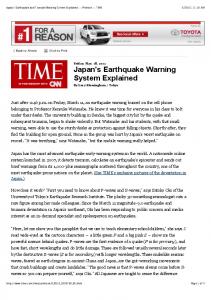
1.2. Japan Since 1952, Japan has been developing its Pacific tsunami warning system. Around Japan there is a network of 300 seismic sensors, including 80 on the seabed, which record seismic activity and water pressure around the clock. Tsunamis are predicted based on the location, strength, and depth below the surface of a quake. A tsunami alert is issued on radio

1.4.2. Short Response Time Although a 10-minute warning is the hoped-for response time, a quake closer to the shore could cut that time dramatically. In a worst-case scenario, according to projections in 2003 by Japan’s Central Disaster Management Council, three simultaneous quakes could generate a magnitude of 8.7,

Improving Tsunami Warning Systems killing 28,000 people, including nearly 13,000 whose lives would be claimed by the resulting tsunami (http://english.aljazeera.net/NR/exeres/4C4B0D4C8598-4000-94F2-4961857C619E.htm).

1.4.3. No System Some poor Asian countries have no tsunami warning system. The sudden and enormous loss of 300,000 lives and property in the December 26, 2004 tsunami affected numerous countries across different continents. GIS and remote sensing have already been widely used in monitoring, predicting, early warning, loss assessment, rescue activities, and aid crisis management for natural disasters. The effectiveness and usefulness of the technologies could be enhanced if they were incorporated into an optimally designed disaster management system.

2. ROLE OF REMOTE SENSING IN THE DECEMBER 26, 2004 INDIAN OCEAN TSUNAMI Remote sensing has been widely used in the December 26, 2004 tsunami’s detection, mapping, monitoring, damage assessment, and crisis management, and would play a large role in an effective warning system due to its “wide and insightful eyesight” in observing similar catastrophic disasters. Examples of remote sensing data and software for the December 26, 2004 tsunami are presented below.

2.1. Remote Sensing Data (1) SPOT (Systeme Pour l’Observation de la Terre) and IKONOS image were used to detect the progression of tsunami waves and sediment change, and to obtain damage details. (2) MODIS (moderate resolution imaging spectroradiometer) band 1 (0.62–0.67 mm) and band 2 (0.841–0.876 mm) (250-m spatial resolution) were used to map coastal flooding. (3) MODIS band 2 was resampled to 500 m for studying sediment load. (4) MODIS-Terra data were acquired less than three hours after the earthquake, and a special emphasis was made to understand trails during propagation and after impact on coastlines.

3 (5) NDVI (normalized differential vegetation index) ratios were used to map tsunami-affected areas. (6) Landsat, RS-1C, 1D, Oceansat-1, and Resourcesat in India were used for analysis and damage assessment. (7) Aerial photography was used by ISRO (Indian Space Research Organisation) to assess the state of agricultural areas, coastal vegetation, and beaches. (8) Orbimage, DigitalGlobe, and Space Imaging provided the U.S. military and National Geospatial-Intelligence Agency with imagery of affected areas for the U.S. Agency of International Development’s Office of Foreign Disaster Assistance on a daily basis. 2.2. Software Two examples of software used in the analysis of remote sensing data for the December 26, 2004 tsunami are presented and we suggest here that GIS and remote sensing software tools are used together to enhance the analysis and efficiency of information processing. (1) ENVI (Environment for Visualizing Images) is a software tool that was used to process and analyze various remote sensing data relevant to the tsunami for a survey of the precursor environment before the tsunami and loss assessment. ENVI provides a flexible framework to integrate the functionality of a GIS such as ARCGIS. (2) ARCGIS is a GIS software that was used to generate a vector layer of the inundated area and the inundated area statistics were computed from this layer. It was also used to help monitor the hazards and make temporal assessments as a guide for logistical services, and help model the hazards as an important data source. 3. DISASTER SYSTEM AND MODELING To investigate quantitatively the potential of remote sensing and GIS in tsunami impact relief, the disaster system (Section 3.1) is decomposed into several components. There are many studies of the components (Petak & Atkinson, 1982; Shi, 1996; Haimes, 2008) and the equations of the essential components are presented in what follows: magnitude of the

4

Wang and Li

ocean

shore

Human activities

MS

Wave

Physical processes

I

could be reduced or eliminated if the link is broken, by displacing humans permanently from the risk area, which could be identified by remote sensing and GIS analysis and records of hazards in history, or by temporal retreat based on professional hazard forecasting, which could be facilitated by remote sensing and GIS, or by expedient escape according to a tsunami warning implemented with remote sensing surveillance. Fig. 2 shows the components of a disaster system and their relationship. Natural hazards causing human and economic losses could be remarkably mitigated by human intervention. “Dissipation measures” (hard intervention) refers to planning flooding zones, releasing rock stress, planting slopes, etc. A society becomes more robust by enhancing buildings to resist earthquakes, relocating houses to noninundation zones to avoid flooding, providing disaster education, and practicing preparation exercises. Relief actions include rescuing buried victims and providing food, water, tents, and medical and sanitary aid. In addition to these concrete and hard measures, losses could also be significantly reduced by “soft” intervention, i.e., monitoring, forecasting, early warning, and evaluating the state and processes of the system components. We modeled the disaster system to evaluate the efficiency of remote sensing and GIS as components

earthquake (the source of tsunami, Section 3.2), intensity of the tsunami (Section 3.3), human society (Section 3.4), and the loss caused by the interactions (bonds) between the hazard and humans (Sections 3.5 and 3.6). The relationships presented are probability models and they are spatially explicit or implicit. Section 4 highlights the nodes of the disaster system where remote sensing and GIS can be embedded to improve the performance of the system. Because our objective is not to provide an integrative software tool or package for modeling the disaster system but, rather, to assess GIS and remote sensing techniques used in a tsunami warning system, the above theories are simplified (Section 5) and then used in calculations. 3.1. Disaster System Natural hazards impact human society through the bond between humans and nature. Humans, nature, and the bond form a disaster system. Fig. 1 shows the disaster system: the top layer represents humans and the bottom layer represents nature. In the case of a tsunami, an earthquake causes wave propagation that forms a destructive tsunami that potentially affects humans on coastlines. As can be seen in this figure, there is a link between humans and the natural hazard (tsunami). Logically, losses

Surveillance Soft intervention

Monitor

Monitor Forecasting

Fig. 1. Hazard propagation (two horizontal arrows) in space and time and impacts on humans (two vertical arrows). The two vertical arrows indicate the linkage between physical processes and human activities, which, like valves, allow the physical impacts on humans to be modified by hard and soft interventions (see Fig. 2). MS stands for the magnitude of the earthquake and I refers to the intensity of the wave after landing.

Monitor Early warning

Evaluation

Fig. 2. Disaster system. Chain

Hard intervention

Input: Hazard

Dissipate energy

System: Society

Robustness

Output: Loss

Relief

Improving Tsunami Warning Systems of the system in disaster relief through their roles in forecasting an event in advance, tracing the progression of the disaster and evaluating the hazard’s spatial impact. Their roles could be further enhanced by the design of an integrated disaster system. 3.2. Magnitude of Hazard: MS As much information and as many indicators as possible are gathered to improve the accuracy and precision of the hazard forecast. These factors, or relevant phenomena, are integrated into a probabilistic, summarized as: MS0 (k) ⇐ P1 (X(i 1 , −τ1 )) ∪ P2 (Z1 (i 2 , −τ3 )), where MS 0 = the magnitude of the earthquake at its epicenter k, X(·) are the factors in the location set {i 1 } that induce MS 0 with a probability P 1 , and Z 1 (·) is a detectable phenomenon at a location set {i 2 } related with X or MS 0 by a probability P 2 , such as the abnormally shaped cloud that was found hovering over Sumatra before the quake, the epicenter of the December 26, 2004 Indian Ocean tsunami earthquake, animal evacuation prior to the hazard, and clusters of rupture movements prior to a major earthquake. The time of earthquake occurrence is given as zero, and τ 1 > 0 and τ 3 > 0 are times ahead of the major quake. The symbol ⇐ denotes probability forecasting and ∪ denotes conjunction. Remote sensing may sense some of X(i 1 , −τ 1 ) and Z(i 2 , −τ 3 ) at places {i 1 } at −τ 1 and {i 2 } at −τ 3 , respectively. Only some types of earthquakes () cause tsunamis: MS(k) = MS0 (k) × δm, where δ m is a switch function, equal to 1 if the MS 0 is a tsunami earthquake, 0 otherwise, based on observations and mechanistic assumptions (some relevant phenomena). MS is what we are interested in. The significance of distinguishing MS 0 and MS is that tsunami prediction based on MS 0 sometimes leads to a false warning. Unfortunately, there is currently little knowledge about δ (McCloskey et al., 2005); consequently, it is not known if δ should trigger the warning system to switch on or off once an earthquake is detected, although there is a statistical relationship (Kulikov et al., 2005). This situation may be overcome if more is understood about the mechanism by which earthquakes trigger tsunamis and if we have more sensors on both the bottom and the surface of oceans.

5 3.3. Intensity of Hazard: I IS ( j, τ5 ) = g(MS(k), d(k, j)) ∪ Z2 (τ5 ); τ5 ( j) = d(k, j)/v; where I S (j, τ 5 ) is the intensity of a tsunami at the shore site j, i.e., the height and speed of the wave of the tsunami, d(k, j) is the distance between the quake epicenter and the front of the wave, g is a function mapping the quake magnitude, distance, and geomorphical features to the height and speed of the wave, Z 2 (τ 5 ) is a natural phenomenon that accompanies I S (t + τ 5 ), such as suspended sediment concentration in the ocean, τ 5 is the time elapsed from the quake (MS) outbreak, and v is the spread velocity of the tsunami wave. Koshimura et al. (2001), Pelinovsky et al. (2002), and Sato et al. (2003) used a deterministic approach and Geist and Parsons (2006) employed probabilistic analysis to specify the formula and parameters. There was remote sensing of Z 2 after the wave landed (http://www.ias.ac.in/currsci/mar102005/709.pdf), and a 10-m-resolution SPOT4 image shows unusually large waves off the coast of Thailand (http://www.spotimage.fr/html/ 167 240 241 781 . php). Water from all inlets J along the shore flooded and accumulated at site i on land, I S in the sea transferred its form to I L , which cost lives and damaged property:  IL(i, τ5 ) = h(IS ( j, τ5 ), w(i, j)) dj ∪ Z3 (τ5 ), J

in which I L (i, τ 5 ) is the depth, area, and duration of flooding. The expression Z 3 (τ 5 ) is a phenomenon that accompanies I L (i, τ 5 ) such as moisture changes on land. The time delay from a tsunami’s arrival at a coastline j to anywhere i on land is very short, so it is omitted here. The term w(i, j) is the pathway from the shoreline inlet j to a site i on land. There is a precise relationship between wave height h on the shoreline and hazard I L on land in hydrology (Matsutomi et al., 2001; Choi et al., 2002), which could be easily acquired from remote sensing and GIS and is a prerequisite of a detailed digital elevation model, and land cover over area {i} just before the arrival of a tsunami. 3.4. Human Society: H Human society, composed of movable and immovable objects, under a hazard risk, is denoted by a human risk matrix H:

6

Wang and Li H(z, m + n | ) ⎛ h1,1 . . . ⎜ ⎜ h2,1 . . . ⎜ =⎜ ⎜ ... ... ⎜ ⎝ hz,1 . . .

h1,m

h1,m+1

...

h2,m

h2,m+1

...

...

...

...

hz,m

hz,m+1

...

h1,m+n

⎞

⎟ h2,m+n ⎟ ⎟ ⎟ ... ⎟ ⎟ ⎠ hz,m+n

= H(M; N | ), where h z ,k refers to the number of the kth type humans or properties distributed over z-level intensity of a risk zone, and z = 1, 2, . . . , z. There are m types of movable objects and n types of immovable properties, and the matrix H accordingly is partitioned into two parts: movable M (left part of the matrix) and immovable N objects (right part of the matrix), which have different vulnerabilities and calculations. The movable objects M (humans, animals) and immovable property N (houses, crops) react differently to condition , i.e., the knowledge of hazards, government regulations, and warnings. The various reactions to  lead to various distributions and adoptions of human society H(M, N) just before a hazard descends.

3.5. Vulnerability: V Vulnerability of human society (H) to hazard intensity (I) is an empirical data matrix V: V(z, m + n) ⎛ v1,1 ⎜ ⎜ v2,1 ⎜ =⎜ ⎜ ... ⎜ ⎝ vz,1

...

v1,m

v1,m+1

...

...

v2,m

v2,m+1

...

...

...

...

...

...

vz,m

vz,m+1

...

v1,m+n

⎞

⎟ v2,m+n ⎟ ⎟ ⎟ ... ⎟ ⎟ ⎠ vz,m+n

= V(M; N), where v z ,k is the percentage loss of a kth type of object under intensity z. V is obtained by empirical regression (Sonmez et al., 2005; Badal et al., 2005; Anderson, 2003; Van Der Voet & Slob, 2007) or engineering experiment. We used observed losses to regress the estimated height of the wave over space to evaluate the values in this article.

3.6. First Loss from Hazard Arrival to Its Physical End: L 0 By multiplying the vulnerability matrix and human risk matrix, we obtain the first loss matrix: L0 (M; N | ) = V(M; N) ⊗ H(M; N | ) ⎧ (0; 0) 6 : H(0; 0), ⎪ ⎪ ⎪ ⎪ ⎪ ⎪ prediction, ⎪ ⎪ ⎪ ⎪ ⎪ knowledge, and ⎪ ⎪ ⎪ ⎪ regulation ⎪ ⎪ ⎪ ⎪ ⎪ (βv(M)h(M); v(N)h(ρ N)) 5 : H(β M; ρ N), ⎪ ⎪ ⎪ ⎪ ⎪ optimal ⎪ ⎪ ⎪ ⎪ warning, ⎪ ⎪ ⎪ ⎪ ⎪ knowledge, ⎪ ⎪ ⎪ ⎪ ⎪ no regulation ⎪ ⎪ ⎪ ⎪ 4 : H(α M; N), ⎪ (αv(M)h(M); v(N)h(N)) ⎪ ⎪ ⎪ ⎪ early warning, ⎨ no knowledge ⎪ ⎪ ⎪ (v(M)h(M); 0) 3 : H(M; 0), ⎪ ⎪ ⎪ ⎪ ⎪ no warning, ⎪ ⎪ ⎪ ⎪ ⎪ knowledge, ⎪ ⎪ ⎪ ⎪ regulation ⎪ ⎪ ⎪ ⎪ ⎪ (v(M)h(M); v(ρ N)h(ρ N)) 2 : H(M; ρ N), ⎪ ⎪ ⎪ ⎪ ⎪ no warning, ⎪ ⎪ ⎪ ⎪ knowledge, ⎪ ⎪ ⎪ ⎪ ⎪ no regulation ⎪ ⎪ ⎪ ⎪ ⎪ (v(M)h(M); v(N)h(N)) 1 : H(M; N), ⎪ ⎪ ⎪ ⎪ no warning, ⎪ ⎪ ⎪ ⎩ no knowledge in which L 0 (M; N | ) is the loss of movable objects M and immovable property N. Knowledge of risk  induces hazard-resistant infrastructure and buildings, ρN < N, where ρ is the percentage of damage; government regulations on hazard management lead to both human and property displacement away from the risk zone; risk warning promotes the retreat of movable objects. In condition 6, there is a prediction of hazard. Therefore, the movable objects M should have enough time for retreat so that none are lost, and the knowledge of hazards and government regulations guarantee that immovable property will be built outside of risk zones so that no immovable property will be lost either. Under the 5 condition, there are no government regulations, and some real estate is built inside risk zones, although buildings may be enhanced to resist hazard to some

Improving Tsunami Warning Systems

7

degree (0 < ρ < 1) according to hazard knowledge. A thorough use of remote sensing and GIS and a highefficiency disaster management system enables the maximum retreat of moveable objects, and the loss is βM, where 0 < β < 1. In condition 4, there is no knowledge of hazards or regulations concerning hazards, and the real estate in risk zones is vulnerable to hazards. However, early warning gives people some time to escape the risk zones, and the loss is αM, 0 < α < 1 and β < α. In condition 3, there is no early warning of hazards, people are completely unaware of the coming catastrophe, and are vulnerable to the hazard v(M)h(M), whereas the knowledge and regulation of hazards is such that the real estate has been built outside the risk zones (Robert et al., 2003). In condition 2, there is no warning, so people are fully vulnerable v(M)h(M) to the coming hazard. There are also no government regulations, so real estate has been built within the risk zones, although the loss may be modified by the owners’ knowledge of a coming hazard v(N)h(ρN). The worst case is 1, in which there is no warning and no foreknowledge, so there are no regulations governing hazards, and both humans and their property are completely vulnerable to disaster. Obviously, 6 : L0 (0; 0) < 5 : L0 (β M; ρ N) < 4 : L0 (α M; N); 





3 : L0 (M; 0) < 2 : L0 (M; ρ N) < 1 : L0 (M; N), where α denotes 6: L 0 (0, 0) < 3: L 0 (M; 0), et al. In more detail, L0 (z, m + n | ) = V(z, m + n) ⊗ H(z, m + n | ) ⎛

v1,1 h1,1

⎜ ⎜v h ⎜ 2,1 2,1 ⎜ ⎜ ⎜ ... ⎝

=

vz,1 hz,1 z

i=1

vi,1 hi,1

...

According to this matrix, loss from a disaster can be evaluated on three scales: Scale 1 :v z,mhz,m, loss of mth type object in zone z; z vi,mhi,m , loss of mth type object in entire Scale 2 : i=1 hazard area; m+n j=1 vz, j hz, j , loss over zth level risk and m+n z zone; Scale 3 : i=1 j=1 vi j hi j ,total loss within the disaster area. If loss on scale 1 is found, the losses on levels 2 and 3 are calculated by summing losses of scale 1. Losses on levels 3 or 2 may be approximately estimated by sampling techniques (Wang et al., 2002) without data at lower levels. Furthermore, with downscaling techniques and prior data, losses on levels 2 or 1 may be estimated once we know the losses on levels 3 or 2, respectively.

3.7. Secondary Loss from the Physical End of a Hazard to the End of Relief Action: βL 0 The losses of some movable and unmovable objects increase even after the physical hazard process reaches an end if the relief actions are not immediate and efficient (Sever et al., 2006; Slotta-Bachmayr, 2005; Kuwata & Takada, 2004). Fig. 3 illustrates schematically an empirical relationship, where τ 2 denotes the delay from hazard arrival to the beginning of relief actions, i.e., the time to identify the location and seriousness of a disaster, and the time to access the target area from the resource site. Remote sensing speeds the identification of the target, thus shortening τ 2 . The expression τ 4 denotes the delay from the time relief efforts begin to the time of rescue. The value β(>0) is an empirical parameter, reflecting the efficiency of relief, and is related to the equipment,

...

v1,mh1,m

v1,m+1 h1,m+1

...

...

v2,mh2,m

v2,m+1 h2,m+1

...

...

...

...

...

...

vz,mhz,m

vz,m+1 hz,m+1

...

z

i=1

vi,mhi,m

z

i=1

vi,m+1 hi,m+1

...

v1,m+n h1,m+1

⎞

⎟ v2,m+n h2,m+1 ⎟ ⎟ ⎟ ⎟ ⎟ ... ⎠ vz,m+n hz,m+n z

i=1

m+n

j=1 m+n

j=1 m+n

v1, j h1, j v2, j h2, j ...

.

vz, j hz, j

j=1

vi,m+n hi,m+n

z m+n

i=1 j=1

vi, j hi, j

8

Wang and Li 4. DISASTER SYSTEM OPTIMIZATION AND REMOTE SENSING AND GIS INPUT

L Lmax

4.1. Efficient Time Interval δ

βL0 L0

Relief delay (δ2 + δ4) Fig. 3. Schematic relationship between disaster loss and relief delay (Fu & Chen, 1995).

experience, size of the rescue action, and food and medical aid. The higher the efficiency, the smaller is β, which is expressed by: L(M; N | τ2 , τ4 ; ) = L0 (M; N | ) × [1 + β(1 − e−(τ2 +τ4 ) )]. If the relief actions are totally inefficient, taking δ2 + δ4 → ∞ in the above equation, the maximum losses after the physical end of a hazard are: Lmax (M; N | ) = L0 (M; N | )(1 + β) = L(M; N | α, δ2 , δ4 ; ). The above general model chain from MS to I to H and finally to L was specified by mechanism, system dynamo language, stochastic process, or Taylor expansion, then calibrated by regression if there were corresponding observed data. A quick estimation was made by a simplification of the modeling and using empirical data, as described in Section 5 in this article.

Time is the most crucial factor in disaster reduction: earlier warning allows enough time for retreat, and timely relief reduces secondary loss. Fig. 4 shows the timing of a tsunami process schematically: an earthquake broke out and is denoted by the origin point of a coordinate system composed by space j, time t (τ 1 or τ 3 denotes the times ahead of the quake of predictions using relevant factors or related phenomena, see Section 3.2), and loss L. The quake triggered a tsunami that took about two hours (τ 5 ) to spread from the origin to shorelines and about a further 10 minutes to hit humans and the property distributed along the coast; it might take about three days (τ 2 ) to identify and approximately assess the losses distributed over the widely impacted areas. In light of this information, massive and efficient disaster relief actions were implemented that lasted about one month (τ 4 ); then recovering actions began, including reconstructing houses, lifelines, and other facilities, and these actions lasted about one year or more. The daily losses caused by the tsunami started from the time of the quake, increased dramatically after the waves hit the shore, and reached a maximum; the daily losses continued to the periods of the instant relief actions and recovering actions. The longer the time τ odd (=α 1 τ 1 + α 3 τ 3 + α 5 τ 5 ), the less the loss L; the shorter the time τ even (=α 2 τ 2 + α 4 τ 4 ), the less the loss L. The various α values reflect that the times in different disaster stages have different importance to the loss L(M, N), and the weights can be estimated from past disaster records.

loss, L

prediction (−τ1 or −τ3) spread, 2h (τ5) attack, 10min reaction delay, 3d (τ2) relief, 1mon (τ4) recovery, 1y

time, t

space, j ocean

land

Fig. 4. Schematic time periods of tsunami process.

Improving Tsunami Warning Systems

Disaster System Components Monitoring Table I. Optimization of Disaster System

9

Current Theory

Disaster forecast

Prior knowledge Classic statistics Data-driven single model Vulnerability

Loss evaluation Relief actions

Single hazard Contingency

Hazard prediction

We define a value called the “efficient time interval,” δ, to represent the efficiency of a disaster system: δ = τodd − τeven . Obviously, the larger the δ values are, the less the losses. Remote sensing and GIS play crucial roles in providing timely detailed and correct information of the hazard and disaster states. Furthermore, a highly efficient disaster system would fully utilize remote sensing and GIS functionalities. 4.2. Optimization of Disaster System We investigated the possibilities of lengthening the efficient time interval δ by optimizing the disaster system using state-of-the-art theories. Table I shows current theories used for disaster components and possible new optimization technologies to improve them. Nowadays, the surveillance network is distributed by prior knowledge (Office of Science & Technology of U.S. President, 2005) or by classical/spatial sampling theories (Cochran, 1977). However, a new spatial sampling theory called the sandwich spatial sampling technique, which quantitatively combines both prior knowledge and prior probability, was proven to be much more efficient than others in designing a surveillance network, and also offered several advantages: (1) it combined remote sensing surface information (a spectrum) from the air and sampling point detailed information on the ground (confirmation) to improve the surveillance efficiency; and (2) it combined fine spatial resolution, but expensive and less frequent images (IKNOIS or QUICKBIRD), and coarse, but frequent (SPOT or MODIS), images to produce a new image with higher resolutions in space and time and spectrum at a lower cost. Some hazards such as earthquakes are too complicated to be modeled, but

Optimization Sandwich sampling (Wang et al., 2002) Early alert (Ramirez & Carlos, 2004)) Data-driven mega model (Wang et al., 1996) Scenarios simulation (Li et al., 2005; Wyss, 2005) Regional integration (Wang et al., 1997) Resources allocation, computer-based planning (Wang et al., 2001; Simonovic & Ahmad, 2005)

thanks to the accumulation of observation, we can use data-driven mega models to filter out several distinct patterns from the observed data that are often a mixture of various mechanisms and factors underlying earthquakes (Wang et al., 1996). With the accumulation of observed and test data and the improvement of computer virtual reality techniques, vulnerability analysis (Petak & Atkinson, 1982) is ready to be implemented by scenario simulations (Li et al., 2005; Wyss, 2005). Departmental and regional studies benefit different groups. If a region is at risk from various hazards, people there are interested in an integrative risk assessment when they choose locations for homes, and are also concerned with individual hazards when buying life and property insurance. A technique based on GIS is now available to map out an integrated zonation that shows the risk at both individual and integrated levels (Wang et al., 1997; Peduzzi et al., 2005). The change in secondary losses to the delay of relief actions varies for living beings, lifeline engineering, real estate, etc., and the composition of the hazard susceptibility varies over space; in addition, the first loss from the first attack of a hazard varies in space; therefore, an optimal and dynamic arrangement of relief resources and computerbased evacuation emergency planning will maximize the reduction of secondary losses (Wang et al., 2001; Simonovic & Ahmad, 2005).

4.3. Remote Sensing and GIS Input Remote sensing and GIS play a critical role in improving the performance of disaster systems in forecasting risk, tracing hazards, evaluating loss, and guiding relief actions. To improve the efficiency of disaster systems, it is necessary to enhance the performance of all of the components, with each component corresponding to more specific remote sensors.

10 By investigating the link of every component of a disaster system with remote sensing and GIS (Leung, 1997) (Fig. 2) and then running a model chain (Section 3), we can compare the difference in system performance between cases with and without remote sensing and GIS data as input, and compare the utility of various resolutions in space and time and the spectrum of images in disaster reduction. Although the task of specifying and calibrating all models in a disaster system remains a challenge for scientists in many fields, it is possible to evaluate quantitatively the role of remote sensing and GIS data in disaster reduction through the efficient time interval δ, which directly reflects the essential characteristics of remote sensing and GIS in providing timely correct and detailed spatial information of a disaster before, during, and after an event. Remote sensing and GIS lengthen τodd and shorten τeven , and hence expand δ, which leads to a rise in evacuation rate of movable objects and,

Wang and Li accordingly, a reduction of losses. The argument is calibrated in the following section. 5. THREE SCENARIOS Fig. 5 shows the pilot area of the primary impact zone (PIZ) in Banda Aceh, Indonesia, the place that received the greatest impact of the December 26, 2004 tsunami. About 30,000 people died and 29,545 houses collapsed or were badly damaged inside the PIZ according to a later survey and statistics (CGI, 2005). The PIZ can be further divided into three zones with different risk levels of both intensity of wave (I in Section 3.3) and population density (human society H in Section 3.4), ranging from high risk close to the seashore to low risk farther away. The risk zone’s boundary is comprehensively determined by the texture and color of the remote sensing images after the disaster (L 0 in Sections 3.6 and 3.7, but accounted for by post hoc survey) (QuickBird,

Fig. 5. Pilot area and risk zones of Banda Aceh, Indonesia (map source: QuickBird, Landsat 7, ETM∗ and SRTM; partial data source: ECJRC, 2005; AIT, 2005; CGI, 2005).

w ave height 6 5

11 Deaths (persons)

wave height (m)

Improving Tsunami Warning Systems 18000 16000 14000

4

12000

3

10000 8000

2

6000

1 4000

0 2000

0

1

2

3 4 5 distance from the beach (km )

0 0

2

3

4

5

6

Damage (billion yen)

Fig. 7. Tsunami wave height vs. observed deaths in Banda Aceh, Indonesia, December 26, 2004. (Data sources: UNEP, 2005; Ahmet et al., 2004; Tierney, 2005; Keith, 2005; Helen, 2005; Quirin, 2005; ADB, 2005.) Death (persons) by flooding 1600

100

TV population rate

90

1400

Typhoon movement forecast started in 1953

80

1200 70 1000

60

Computer-based forescast started in 1959 800

50

Percentrate rate of TV (%)

Landsat 7, ETM and SRTM; partial data source for this map’s production—ECJRC, 2005; AIT, 2005; CGI, 2005). We simulated three damage scenarios for the December 26, 2004 Indian Ocean tsunami disaster using three assumptions: (1) scenario 1, without an early warning system, i.e., the current situation, 1 in L 0 (M; N | ) described in Section 3.5; (2) scenario 2, with a system like the existing Pacific Ocean tsunami warning system, 4 in L 0 (M; N | ) in Section 3.5; and (3) scenario 3, with an optimized disaster system fully using remote sensing and GIS as indicated in Table I, 5 in L 0 (M; N | ) in Section 3.5. Fig. 6 shows the intensity of the tsunami as it progresses (intensity I in Section 3.3). The intensity is measured by wave height: the higher the wave, the more destructive power it has. The wave height decreases as the distance from the shoreline increases. It took 10 minutes for the tsunami to travel from the earthquake epicenter to the PIZ shoreline, and 20 minutes to reach the entire PIZ. The curve is based on the actual sample measurement of the tsunami that occurred in Banda Aceh, Indonesia, December 26, 2004 by a field survey and reports (UNEP, 2005; Ahmet et al., 2004; Tierney, 2005; Keith, 2005; Helen, 2005; Quirin, 2005; ADB, 2005) and spatial interpolation (Atkinson, 2005; Penning-Rowsell et al., 2005). Fig. 7 establishes the relationship of numbers of deaths to the wave height of the tsunami (vulnerability V in Section 3.5) through regression using observations. Due to the decrease in wave height with increasing distance from the shore, the number of deaths is positively correlated to the wave height and negatively correlated to the shore distance. After hit-

1

Wave height(m)

Death(persons)

Fig. 6. Tsunami wave height in Banda Aceh, Indonesia, December 26, 2004. (Data sources: UNEP, 2005; Ahmet et al., 2004; Tierney, 2005; Keith, 2005; Helen, 2005; Quirin, 2005; ADB, 2005.)

40

600

Usage of GIS and RS started in 80s 30

400 20 200

10

0

0 1950

1955

1960

1965

1970

1975

1980

Timeline (year)

Fig. 8. Technology development and disaster reduction (statistics on flooding, Hirok, 2005; Ramirez & Carlos, 2004).

ting the shore, the power of the wave decreases with increasing distance from the shore due to the hampering effect of the shore and reduction of the kinetic energy that results in less destructivity and thus fewer deaths. Fig. 7 also shows the number of deaths increases gradually with increasing wave height up to 3 m, above which a rapid increase in deaths occurs. Fig. 8 is adapted from Hiroki (2005). Based on statistics, the figure indicates that each use of new technology (from the 1953 typhoon forecast system to 1959 computer-based forecasting to the 1980s GIS and RS data) were critical points at which the loss (deaths caused by flooding) dropped drastically. The historic assessment of the contributions of the techniques to rescue efficiency (Fig. 8), together with

Evacuation Rate

12

Wang and Li

1.0

0

2

4

6

8

10 1.0

0.8

0.8

Scenario3 0.6

0.6

Scenario2 0.4

0.4

0.2

0.2

Scenario1

0.0 0

10

20

30

40

Fig. 9. Evacuation rates increase with increase of efficient time interval δ in three scenarios (partial sources: Kenzo, 2005; AIT, 2005; Yamazaki, 2001; ECJRC, 2005).

0.0 50

Efficient Time Interval δ (minutes)

other simulated results (AIT, 2005; ECJRC, 2005) and the extrapolation of this trend, demonstrates the effectiveness and contribution of GIS and remote sensing technologies, and also indicates the potential contribution of optimal technology proposed by this article. From Fig. 8, the timing efficiency could be improved by a factor of about 1–2 with the warning system and by a factor of about 3–4 with the warning system optimized with GIS and remote sensing techniques. The values of these improvements (Fig. 8) were used to simulate the evacuation rates corresponding to the critical timing points under scenarios 2 and 3, whereas scenario 1 is the factual situation of the 2004 Indonesian tsunami from surveys. The loss (L 0 in Section 3.6) is negatively proportional to the evacuation rates of objects, whereas the latter is positively proportional to δ. As for movable humans, the evacuation rates (including time coefficients) in Fig. 9 were firstly acquired at critical points from the arrival of the tsunami to 45 minutes later from survey reports (Kenzo, 2005; AIT, 2005; Yamazaki, 2001; ECJRC, 2005), then the points were regressed and extrapolated to produce curves, considering Fig. 8, GIS and remote sensing application experience, human physical potentials, and the local transportation situation. We acknowledge that there exists some arbitrariness in the estimation of the disaster parameters due to the nonrepeatability of the event that cannot be experimentally investigated, but the uncertainty is mitigated by Fig. 8 and studies

by Kenzo (2005), AIT (2005), Yamazaki (2001), and ECJRC (2005). From Fig. 9, it can be seen that without any warning system (scenario 1), the evacuation is slow and ineffective, and there were many people who had still not been evacuated 50 minutes after the tsunami caused the most damage (as the scenario 1 plot indicates). This was the actual condition in the Banda, Aceh disaster. With a warning system similar to the existing Pacific tsunami system, the evacuation is effective. Under this scenario, after 15 minutes, the evacuation rate starts to increase until 35 minutes, at which time all people have been evacuated. The damage from the tsunami is assumed to be partial and moderate in this scenario. Furthermore, the plot for scenario 3 indicates the evacuation is timely and effective and all components relevant to before, during, and after the disaster in the disaster system were optimized as shown in Table I using GIS and remote sensing as inputs. Ten minutes after the tsunami’s occurrence, the rescue activity would be initiated (Ramirez & Carlos, 2004). We assume that people can be completely evacuated, with few losses, within 20 minutes under this scenario. In summary, the proportions of evacuation rates under the three scenarios 1, 2, and 3 corresponding to the efficient time interval δ are roughly 0, 0.5, and 1, respectively. With the above parameters, we projected disaster scenarios in three distinct technical conditions. The results are summarized in Table II. The loss rate

Improving Tsunami Warning Systems is determined by the vulnerability and the amount of property (including humans and houses). The human loss rate and loss amount decreases from scenarios 1 to 3 and from A (high risk), to B (mid risk) to C (low risk). The housing loss rate has slight differences in that the effects of  are not considered. Therefore, the housing loss risk is the same in each risk zone, but decreases from A to B to C under each scenario. Each risk zone corresponds to z in the equation H(z, m + n | ) in Section 3.5. In summary, there are four risk levels and so z = 4. Here, only humans are considered as movable objects and hence m = 1. Similarly houses are included in the immovable object group, and so n = 1.  corresponds to three different conditions (i.e., the scenarios in the first rows of Table III, scenarios 1–3): no knowledge and no warning, knowledge and warning, and knowledge and warning with optimal technologies using GIS and remote sensing as inputs; then, the losses were estimated by the equation L 0 (M; N | ) = v(M; N) ⊗ h(M; N | ) in Section 3.5. 5.1. Scenario 1 We first estimated the rates of the number of dead and missing persons among the total population in the PIZ. Let L z be the number of deaths in a certain zone z, h z be the number of residents in z, and I z the intensity of the disaster in z. For simplification of the simulation, we assume the vulnerability of human society to a tsunami is proportional to the hazard intensity. This assumption is rational because a very intense hazard results in much greater loss (Shi, 1996). Therefore, we use the following equation to simplify that in Section 3.5 for our simulation: Lz = vz × hz = g × Iz × hz, where v z is the vulnerability of human society to a tsunami under various circumstances of  (Section 3.6), and is proportional to I z by a coefficient γ . The vulnerability coefficient γ involves the intensity (wave height) and the vulnerability of human society under different technical conditions (scenarios) and helps build the relationships among intensity (I z ), death (the human loss, L z ), and population (h z ). For h z , an even distribution of the population over the PIZ is assumed: h A = h × (1.8/4.7), h B = h × (1.5/4.7), hC = h × (1.4/4.7),

13 where h is the total number of residents in the PIZ, and 1.8 + 1.5 + 1.4 = 4.7 km are the mean widths of A, B, and C and the PIZ measured in Fig. 5. For I z , the intensity of a tsunami is described by its wave height, and is obtained from Fig. 6: IA = 4.5 ∼ 6m, IB = 2 ∼ 4.5m, IC = 0 ∼ 2m. Consequently, LA : LB : LC = 18 × (4.5 ∼ 6) : 15 × (2 ∼ 4.5) : 14 ×(0 ∼ 2) ≈ 55% : 30% : 15%. For houses, the proportion of collapsed structures between the zones is assumed to be similar to the human death proportion. The proportions and total deaths M and the number of collapsed and seriously damaged houses N in the PIZ were estimated for each of the risk zones in scenario 1, as listed in Table II. 5.2. Scenarios 2 and 3 From the curves in Fig. 9, the proportions of the loss rates under the three scenarios are found to be 10:5:1 or 1:0.5:0.1 (the evacuation rate is 1:5:10) for movable humans. For immovable real estate, the relationship is simply 1:1:1 due to ’s limited effect upon the loss of houses; i.e., there are similar loss rates under different scenarios. Using the models described in Section 3.6, we estimated the deaths in PIZ in scenarios 2 and 3 to be 15,000 and 3,000, respectively, based on the survey data of 30,000 deaths in scenario 1. By two largely rational assumptions that the proportions of losses between A, B, and C remain unchanged in 1, 4, and 5, and that the losses stay the same for immovable objects under the three technological conditions, we easily obtain the remaining figures in Table II. 6. CONCLUSIONS AND DISCUSSION The merits of GIS and remote sensing in disaster relief could be enhanced in an optimized disaster system. We measured their potential contribution in disaster reduction through an indicator called the efficient time interval by modeling a disaster system and simulating its performance under three conditions. Under the assumption of a tsunami attack with the same intensity as that of the December 26, 2004 Indian Ocean tsunami, the simulations in the PIZ in Banda Aceh, Indonesia, disclosed quite different scenarios for the losses of human life and houses in

14

Wang and Li Table II. Summaries of Three Damage Scenarios of the Tsunami Under Three Technological Conditions Scenario 1 L(M, N | 1)

Zones A

B

C

Sum

Deaths (persons)

Rate

>55%

Houses collapsed and damaged badly

Number Rate Number

>16,500 >55% >16,249

Deaths (persons)

Rate

30–55%

Houses collapsed and damaged badly

Number Rate Number

9,000–16,500 30–55% 8,863–16,249

Deaths (persons)

Rate

15–30%

Houses collapsed and damaged badly

Number Rate Number Rate Number Rate Number

Deaths (persons) Houses collapsed and damaged badly

Scenario 2 L(M, N | 4)

Scenario 3 L(M, N | 5)

>55% × 0.5 = 27.5% >8,250 55% >16,249

>55% × 0.1 = 5.5% >1,650 55% >16,249

30–55% × 0.5 = 15–27.5% 4,500–8,250 30–55% 8,863–16,249

30–55% × 0.1 = 3–5.5% 900–1,650 30–55% 8,863–16,249

4,500–9,000 15–30% 4,431–8,863

15–30% × 0.5% = 7.5–15% 2,250–4,500 15–30% 4,431–8,863

15–30% × 0.1% = 1.5–3% 450–900 15–30% 4,431–8,863

100% 30,000 100% 29,545 (80% of BA)

100% × 0.5 = 50% 15,000 100% 29,545 (80% of BA)

100% × 0.1 = 10% 3,000 100% 29,545 (80% of BA)

Note: BA refers to Banda Aceh; Rate = L(M; N) in zone z/H(M; N) in zone z.

different conditions: scenario 1 with no warning system at all, which is the same as the current situation, scenario 2 with a warning system like that currently serving in the Pacific Ocean, and scenario 3 under the proposed optimized warning system fully using GIS and remote sensing. The idea of disaster reduction that implements remote sensing and GIS into an optimized tsunami warning system is that the technology shortens the delay of an early warning and assessment of the risk while lengthening the period for evacuation, and more accurate information of the location and severity of the disaster is provided. Remote sensing is used to improve the accuracy of the data and to speed data gathering and information processing. GIS provides a platform to deal with and integrate various geospatial data and is used to implement its functionalities with other modules. ENVI is used to deal with remote sensing data to extract relevant information for statistical analysis. The probabilistic or mathematical models (e.g., magnitude of earthquake, intensity of tsunami, assessment of primary, and secondary losses caused by a tsunami and resulting disasters) are implemented by Matlab, SPSS, and SAS. In our simulation, we obtained Fig. 5 using GIS and RS materials and maps and estimated the timing efficiency using

GIS and RS (scenario 3). The efficiency of GIS and RS techniques in relief timing can be improved corresponding to scenario 3 and L(M, N | 5). The parameters of the procedure were calibrated, which gave an estimation of the losses for three different levels of technologies. Using the data and materials of the Indian tsunami on December 26, 2004, a simulation was performed. The factual situation without a tsunami warning system caused a great number of deaths (30,000). The simulation showed that a warning system similar to that in the Pacific could halve the number of deaths (15,000; see Table II). However, if equipped with sophisticated GIS, remote sensing, and optimization techniques, the warning system, as the simulation shows, could reduce number of deaths to 3,000. Our comparison and conclusion have significant implications for planning, building, and optimization of a tsunami warning system. The proposed optimized disaster system should be equipped with stateof-the-art instruments and advanced theories relevant to disasters. GIS and remote sensing could be implemented into every node of the system from forecasting, monitoring, and early warning to assessing, regulating, and intervening, and this would considerably relieve the impact of a tsunami hazard.

Improving Tsunami Warning Systems ACKNOWLEDGEMENTS This study is supported by the NSFC (70571076, 40471111, 40601077), MOST (2006AA12Z215, 2007AA12Z233, 2007DFC20180), and CAS (KZCX2-YW-308).

REFERENCES ADB (Asian Development Bank). (2005). An Initial Assessment of the Impact of the Earthquake and Tsunami of December 26, 2004 on South and Southeast Asia (report). Available at http://www.adb.org/Documents/Others/Tsunami/impact earthquake tsunami.pdf. Ahmet, C., Dogan, P., Sukru, E., et al. (2004). December 26, 2004 Indian Ocean Tsunami Field Survey at North Sumatra Island (a survey report). Available at http://www.ioc. unesco.org/iosurveys/Indonesia/yalciner/htm. AIT (Asian Institute of Technology). (2005). Working Papers on AIT’s Response to the Earthquake and Tsunami in South and Southeast Asia (a collection of papers). Available at http://www.tsunami.ait.ac.th/Documents/AIT Tsunami Paper.pdf. Anderson, L. (2003). Community vulnerability to tropical cyclones: Cairns, 1996–2000. Natural Hazards, 30, 209–232. Atkinson, P. (2005). Spatial prediction and surface modeling. Geographical Analysis, 37, 113–123. Badal, J., Vazquez-Prada, M., & Gonzalez, A. (2005). Preliminary quantitative assessment of earthquake casualties and damages. Natural Hazards, 34, 353–374. Bernard, E. (2005). The U.S. National Tsunami Hazard Mitigation Program: A successful state–federal partnership. Natural Hazards, 35, 5–24. CGI (the Consultative Group on Indonesia). (2005). Indonesia: Preliminary Damage and Loss Assessment (The December 26, 2004 Natural Disaster) (a survey report). Available at http://www.undp.org/cpr/disred/documents/tsunami/indonesia/ reports/damage assessment0105 eng.pdf. Choi, B., Pelinovsky, E., Ryabov, I., & Jin, S. (2002). Distribution functions of tsunami wave heights. Natural Hazards, 25, 1–21. Cochran, W. (1977). Sampling Techniques, 2nd ed. New York: John Wiley & Sons Inc. ECJRC (European Commission Joint Research Centre). (2005). Preliminary Damage Assessment and Information Reporting During the Earthquake and Subsequent Tsunami Disaster in the Indian Ocean (Version of Debriefing Note) (report). Available at http://tsunami.jrc.it/Reports/Tsunami11 Jan 10vWebJRC.pdf. Fu, C., & Chen, X. (1995). Seismic risk zonation of China. In J. Wang (Ed.), Regionalization of Hazards in China. Beijing: China Science & Technology Press. Geist, E., & Parsons, T. (2006). Probabilistic analysis of tsunami hazards. Natural Hazards, 37, 277–314. Haimes, Y. Y. (2008). Risk Modeling, Assessment, and Management, 3rd ed. New Jersey: John Wiley & Sons. He, J., Tian, G., & Wang, J. (1993). Progress of Monitoring and Evaluating Natural Disasters Using Remote Sensing. Beijing: China Sciences & Technology Press. Helen, P. (2005). Scientists seek action to fix Asia’s ravaged ecosystems. Nature, 433, 94. Hiroki, H. (2006). Early Warning. Presented at the World Conference on Disaster Reduction. Kobe, Japan. Available at http://www.unisdr.org/wcdr/thematic sessions/cluster2.htm.

15 Keith, A. (2005). Watching over the world’s oceans. Nature, 434, 19–20. Kenzo, H. (2005). Early Warning, Ministry of Land, Infrastructure and Transport, Japan (report). Koshimura, S., Imamura, F., & Shuto, N. (2001). Characteristics of tsunamis propagating over oceanic ridges: Numerical simulation of the 1996 Irian Jaya earthquake tsunami. Natural Hazards, 24, 213–229. Kulikov, E., Rabinovich, A., & Thomson, R. (2005). Estimation of tsunami risk for the coasts of Peru and northern Chile. Natural Hazards, 35, 185–209. Kuwata, Y., & Takada, S. (2004). Effective emergency transportation for saving human lives. Natural Hazards, 33, 23–46. Leung, Y. (1997). Intelligent Spatial Decision Support System. Berlin and New York: Springer Verlag. Li, L., Wang, J., & Wang, C. (2005). Typhoon insurance pricing with spatial decision support tools. International Journal of Geographical Information Science, 19(3), 363–384. Matsutomi, H., Shuto, N., Imamura, F., & Takahasgi, T. (2001). Field survey of the 1996 Irian Jaya earthquake tsunami in Biak Island. Natural Hazards, 24, 199–212. McCloskey, J., Nalbant, S., & Steacy, S. (2005). Earthquake risk from co-seismic stress. Nature, 434, 291. Office of Science & Technology of U.S. President, Executive Office of the President. (2005). Strategic Plan for the U.S. Integrated Earth Observation System. Available at http://www.ostp.gov/html/EOCStrategic˙Plan.pdf. Peduzzi, P., Dao, H., & Herpld, C. (2005). Mapping disastrous natural hazards using global datasets. Natural Hazards, 35, 265– 289. Pelinovsky, E., Kharif, C., Riabov, I., & Francius, M. (2002). Modelling of tsunami propagation in the vicinity of the French coast of the Mediterranean. Natural Hazards, 25, 135– 159. Penning-Rowsell, E., Floyd, P., Ramsbottom, D., & Surendran, S. (2005). Estimating injury and loss of life in floods: A deterministic framework. Natural Hazards, 36, 43–64. Petak, W., & Atkinson, A. (1982). Natural Hazard Risk Assessment and Public Policy Anticipating the Unexpected. Berlin: Springer-Verlag. Quirin, S. (2005). On the trail of destruction. Nature, 433, 350–353. Ramirez, F., & Carlos, P. (2004). The local tsunami alert system [“SLAT”]: A computational tool for the integral management of a tsunami emergency. Natural Hazards, 31, 129– 142. Robert, B., Forget, S., & Rousselle, R. (2003). The effectiveness of flood damage reduction measures in the Montreal region. Natural Hazards, 28, 367–385. Sato, H., Murakami, H., & Kozuki, Y. (2003). Study on a simplified method of tsunami risk assessment. Natural Hazards, 29, 325– 340. Sever, M., Vanholder, R., & Lameire, N. (2006). Management of crush-related injuries after disasters. New England Journal of Medicine, 254, 1052–1063. Shi, P. J. (1996). Theory and practice of disaster study. Journal of Natural Disasters (in Chinese), 5(4), 6–17. Simonovic, S., & Ahmad, S. (2005). Computer-based model for flood evacuation emergency planning. Natural Hazards, 34, 25–51. Slotta-Bachmayr, L. (2005). How burial time of avalanche victims is influenced by rescue method: An analysis of search reports from the Alps. Natural Hazards, 34, 341–352. Sonmez, F., Komuscu, A., Erkan, A., & Turgu, E. (2005). An analysis of spatial and temporal dimension of drought vulnerability in Turkey using the standardized precipitation index. Natural Hazards, 35, 243–264. Tierney, K. (2005). Effective Strategies for Hazard Assessment and Loss Reduction: The Importance of Multidisciplinary and

16 Interdisciplinary Approaches (Report from Internet). Available at http://www.ncdr.nat.gov.tw/chinese/download/ paperTierney/pdf. UNER (United Nations Environment Programme). (2005). After the Tsunami: Rapid Environmental Assessment. Available at http://www.unep.org/tsunami/reports/TSUNAMI report complete.pdf. Van Der Voet, H., & Slob, W. (2007). Integration of probabilistic exposure assessment and probabilistic hazard characterization. Risk Analysis, 27, 351–371. Wang, J. F. (Ed.). (1993). Methodology for Assessing Natural Disaster Risk in China. Beijing: China Science & Technology Press. Wang, J. F., & Li, Q. L. (1996). Adaptive structure model of earthquake trend regionalization. Earthquake Research in China, 12, 78–88.

Wang and Li Wang, J. F., Liu, C. M., Wang, Z. Y., & Yu, J. J. (2001). A marginal benefit model for distributing water resources in space. Science in China (Series D), 31(5), 422–427. Wang, J. F., Liu, J. Y., Zhuan, D. F., Li, L. F., & Ge, Y. (2002). Spatial sampling design for monitoring cultivated land. International Journal of Remote Sensing, 23(2), 263–284. Wang, J. F., Wise, S., & Haining, R. (1997). An integrated regionalization of earthquake, flood and drought hazards in China. Transactions in GIS, 2(1), 25–44. Wyss, M. (2005). Human losses expected in Himalayan earthquakes. Natural Hazards, 34, 305–314. Yamazaki, F. (2001). Applications of remote sensing and GIS for damage assessment. In R. B. Corotis, G. I. Schueller, & M. Shinozuka (Eds.), Structural Safety and Reliability (report). Lisse/Abingdon/Exton(PA)/Tokyo: A. A. Balkema Publishers.