of the identification method and designing a controller to track a desired ZMP .... C1 = I2 â C. (8). I2 is the identity matrix of dimension two and â is the operator.
Improving ZMP-based Control Model Using System Identification Techniques Wael Suleiman, Fumio Kanehiro, Kanako Miura and Eiichi Yoshida CNRS-AIST JRL (Joint Robotics Laboratory), UMI3218/CRT Intelligent Systems Research Institute National Institute of Advanced Industrial Science and Technology (AIST) Tsukuba Central 2, 1-1-1 Umezono, Tsukuba, Ibaraki, 305-8568 Japan {wael.suleiman, f-kanehiro, kanako.miura, e.yoshida}@aist.go.jp
Abstract—The approximation of humanoid robot by an inverted pendulum is one of the most used model to generate a stable motion using a planned Zero Moment Point (ZMP) trajectory. In this paper, we aim at proposing to improve the reliability of this model using system identification techniques. To achieve this goal, we propose an identification method which is the result of the comprehensive application of system identification to dynamic systems. Moreover, we propose a controlling algorithm for the identified model in oder to track a desired trajectory of ZMP. The efficiency of the method is shown using dynamical simulation and conducting real experiments on the humanoid robot HRP-4C. Index Terms—Humanoid robot; ZMP control; System identification; Optimization; Nonlinear system control
I. I NTRODUCTION Research on biped humanoid robot is nowadays one of the most active research fields in robotics. Making the humanoid robots walk was the subject of intense investigation last years. Many researchers have proposed different methods to generate a stable walking motion for humanoid robot [1]–[5]. Almost of these methods are using a simplified model which it is based on the approximation of the humanoid robot by an inverted pendulum model. The mass of inverted pendulum coincide with the Centre of Mass (CoM) of the humanoid robot. In order to generate a stable motion (dynamically balanced), these methods use the principle of Zero Moment Point (ZMP) [6]. The ZMP is a point of the support polygon (i.e. the convex hull of all points of contact between the support foot (feet) and the ground), at which the horizontal moments are vanishing. The cart-table model proposed by Kajita et al [3] is one of these methods. The efficiency of this method has been proved by generating online stable walking motions using a planned trajectory of ZMP. The purpose in this paper is to show that the linear model related to cart-table model can be improved by capturing the dynamic difference between the response of cart-table model and the ZMP of the multibody model of the humanoid robot, then identifying a quadratic system [7] able to approximate this difference. The paper is organized as follows. Section II gives the kinematic structure of the humanoid robot HRP-4C which is used to validate the proposed method. An overview of the carttable model and the proposed model to improve the reliability
of the cart-table model is discussed in Section III. An adapted identification method for the proposed model is developed in Section IV. Section V points out the implementation algorithm of the identification method and designing a controller to track a desired ZMP trajectory. The efficiency of the proposed model is shown in Section VI through real experiment on the humanoid robot HRP-4C [8]. II. H UMANOID ROBOT: K INEMATIC S TRUCTURE The proposed method is validated using a humanoid robot HRP-4C [8]. HRP-4C is a life-size humanoid robot which was developed for the entertainment use such as a fashion model, master of ceremony of various events and so on. For these applications, it has been decided to make it more humanlike than the humanoid robots that have developed so far [9], [10]. In order to realize a humanlike shape, its dimensions are designed referring to a database of Japanese women of 20’s [11]. As a result, HRP-4C has a humanlike shape as shown in Fig.1(left). The basic specifications and joint configurations are shown in Table I and Fig.1(right) respectively (Face and hand joints are not displayed).
Fig. 1: Exterior and joint configuration of Humanoid Robot HRP-4C (Face and hand joints are not displayed)
m¨ x
TABLE I: Specifications of HRP-4C
degrees of freedom
height weight(including batteries) sensors
arm hand leg waist neck face total
6 2 6 3 3 8 42 158[cm] 43[kg] force/torque sensor×2, inertia sensor
mg zc
τZMP O III. C ART- TABLE M ODEL A ND T HE P ROPOSED M ODEL The main idea of cart-table model [3] is to approximate the humanoid robot by a mass located at its Center of Mass (CoM ) and it is equal to the total mass of the humanoid robot. Therefore, the complex problem of controlling the humanoid robot is transformed to control an inverted pendulum. Let us define the Cartesian position of the center of mass (PCoM ) by x PCoM = y (1) zc
We suppose that the vertical position of the mass zc is constant. The ZM P is a particular point of the horizontal plane at which the horizontal moments vanish. For the inverted pendulum, it is defined as follows # � � " ¨ x − zgc x px (2) ZM P = = y − zgc y¨ py where g is the absolute value of gravity acceleration. It is clear from (2) that the two elements of ZM P are very similar. For that, in the sequel, we figure out how to build the control model for px . To control px , Kajita et al [3] proposed to consider the cart table model, which is shown in Fig. 2. It depicts a running cart of mass m on a pedestal table whose mass is negligible. In our case, this mass is equal to the total mass of the humanoid robot and its center coincides with the CoM of humanoid robot. 1) Controlling ZMP: Let us define a new variable ux as the time derivative of x ¨ ux =
d¨ x dt
(3)
The variable ux is usually called the jerk. Regarding ux as the input of px , we can translate the equation of px into the following dynamical system x 0 1 0 x 0 d x˙ = 0 0 1 x˙ + 0 ux dt x ¨ 0 0 0 x ¨ 1 (4) h i x px = 1 0 − zgc x˙ x ¨
px x Fig. 2: Cart-table model
As the humanoid robot is controlled in discrete time, we discretize the system (4) with sampling time Ts , the control model for px can be expressed by the following formula
zk = Azk−1 + B u ¯k pk = Czk
(5)
where � �T ˙ ¨(kTs ) zk , x(kTs ) x(kT s) x
u ¯k , ux (kTs )
pk , px (kTs ) 1 Ts Ts2 /2 Ts A = 0 1 0 0 1 3 Ts /6 B = Ts2 /2 Ts i h C = 1 0 − zgc
(6)
Regarding the similarity of the equations of px and py , the above equation can be extended to obtain the ZMP based control model as follows
1 Xk1 = A1 Xk−1 + B1 uk
pk = C1 Xk1
(7)
The obtained model is a quadratic system in the state space representation. This realization of quartic system is given by the following structure
where
x(kTs ) x(kT s ) ˙ x ¨ (kT ) s Xk1 , y(kTs ) , y(kT ˙ s) y¨(kTs )
� � ux (kTs ) , , uy (kTs )
uk
A1 = I2 ⊗ A
B1 = I2 ⊗ B C1 = I2 ⊗ C
(8) I2 is the identity matrix of dimension two and ⊗ is the operator of Kronecker product which is defined as follows: X ∈ Rm×n , Y ∈ Rp×l : x11 Y · · · x1n Y . .. .. . (9) X ⊗ Y ∈ Rmp×nl , . . . xm1 Y · · · xmn Y th
th
where xij is the element of the i line and the j column of the matrix X. The above model has been used to generate a stable biped waking patterns using preview controller [3]. However, when the error between the output of this model and that one the real ZMP trajectory of the humanoid robot becomes bigger than the stability margin the robot will fall down. The solution proposed by Kajita [3] is to inject this error in the preview controller as a second stage in order to eliminate the dynamic error. However, this procedure require the dynamic simulation of the multi-body model of the humanoid robot, as a result it is a time consuming process. To overcome this problem, we propose to model the ZMP of the humanoid robot by the model given in Fig. 3. This model consists of two blocks, the first one is the previous cart-table model and the second one is a linear system with respect to the input uk ⊗ Xk1 . The main objective of the second block is to capture the dynamic behavior related to the difference between the simple cart-table model and the multi-body model of the humanoid robot.
Cart-Table Model
uk
1 Xk1 = A1 Xk−1 + B1 uk
yk1
=
1 Xk1 = A1 Xk−1 + B1 uk
� � px (kTs ) pk , py (kTs )
+
C1 Xk1
Xk1 ! " 2 Xk2 = A2 Xk−1 + B2 uk ⊗ Xk1 yk2 = C2 Xk2
Fig. 3: Proposed ZMP model
+
ZM P
2 Xk2 = A2 Xk−1 + B2 (uk ⊗ Xk1 )
pk =
C1 Xk1
+
(10)
C2 Xk2
where uk ∈ R2 is the input signal of the system expressed as 2 in �Eq. (8). pk ∈ R is the output of the system (ZMP).1 i : Xk i = 1, 2 are the states, the dimension of Xk is 6, and the dimension of Xk2 is n2 that will be determined by the identification algorithm. We have proven [7], [12] that this class of nonlinear system is a special case of Volterra series of degree two. This class can play a useful role to model many real systems in practice. The direct relation between pk and uk can be obtained by using the property F G ⊗ HJ = (F ⊗ H) (G ⊗ J) and a simple development of (10) pk =
k P
i=1
Φ1 (k, i)ui +
k i P P
i=1 j=1
Φ2 (k, i, j)(ui ⊗ uj )
where Φ1 (k, i) = C1 (A1 )k−i B1
(11)
h �i Φ2 (k, i, j) = C2 (A2 )k−i B2 I2 ⊗ (A1 )i−j B1 IV. S YSTEM I DENTIFICATION
It is clear that the system is defined by the coefficient matrices of Structure (10). The unknown matrices are A2 , B2 and C2 . That means that the structure parameters can be given by vec(A2 ) θ = vec(B2 ) (12) vec(C2 ) where vec(.) denotes the vectorization operator defined as follows vec : M ∈ Rm×n → Rm·n � � h vec(M ) = vec m1 m2 · · · mn = mT1
mT2 · · · mTn
iT
Given the input uk and the output pk of the real system, our goal is achieved if the output of the following model ˆ 1 = A1 X ˆ 1 + B1 uk X k k−1 2 2 ˆ ˆ k−1 ˆ k1 ) Xk (θ) = A2 (θ)X (θ) + B2 (θ)(uk ⊗ X
(13)
ˆ k1 + C2 (θ)X ˆ k2 (θ) pˆk (θ) = C1 X
approximates the output pk of the real system accurately enough. This criterion can be transformed into the minimization of the output error with respect to the parameters θ. Considering a data length equal to N , the output-error cost function is given by
N
1 X
pk − pˆk (θ) 2 = 1 EN (θ)T EN (θ) (14) 2 N N k=1 � �T where EN (θ) = e(1)T e(2)T · · · e(N )T is the error vector in which e(k) = pk − pˆk (θ). The minimization of (14) is a nonlinear, nonconvex optimization problem. The numerical solution of this problem can be calculated by different algorithms. For instance, the gradient search method is a popular one. This iterative method is based on the updating of the system parameters θˆ as follows T ˆi−1 T ˆi−1 θˆi = θˆi−1 −(ψN (θ )ψN (θˆi−1 )+λi I)−1 ψN (θ )EN (θˆi−1 ) (15) Where λi is the regularization parameter and
∂EN (θ) ∂θT is the Jacobian of the error vector EN (θ). ψN (θ) ,
(16)
A. Multiple Experiments Identification In fact the model obtained by considering a single experiment might be not reliable [13]. This is because the input signals are not perfectly excited. To overcome this problem in identifying practical applications, we apply various sets of input signals. The objective of each set is exciting one or more modes of the system. The multiple experiments should be exploited simultaneously to obtain an accurate model of the system. The optimization problem which consider K experiments simultaneously can be formulated as follow Ni K
2 1 X 1 X 1
i
JK (θ) =
pk − pˆik (θ) = EK (θ)T EK (θ) K i=1 Ni K 2 k=1 (17) where h iT 1 2 K EK (θ) = EN (θ)T EN (θ)T · · · EN (θ)T (18) 1 2 K
and
iT 1 h i T i T i e (1) e (2) · · · ei (Ni )T EN (θ) = √ i Ni
(19)
is the error vector in which ei (k) = pik − pˆik (θ). pik is the output of the system according to the input uik . The estimated output pˆik (θ) of the data set number i is given by the following model ˆ 1,i = A1 X ˆ 1,i + B1 uik X k k−1 ˆ 2,i (θ) = A2 (θ)X ˆ 2,i (θ) + B2 (θ)(uik ⊗ X ˆ 1,i ) X k
pˆik (θ)
k−1
ˆ 1,i + C2 (θ)X ˆ 2,i (θ) = C1 X k k
k
(20)
The minimization of (17) can be calculated, similarly to the case of single experiment, by using the recursive gradient search method as follows T ˆl T ˆl θˆl+1 = θˆl − (ψK (θ )ψK (θˆl ) + λl I)−1 ψK (θ )EK (θˆl ) (21)
where
JN (θ) =
and
ψK (θ) = i ψN (θ) , i
1 ψN (θ) 1 2 ψN (θ) 2 .. . K ψN (θ) K i ∂EN (θ) i ∂θT
(22)
(23)
i is the jacobian of the error vector EN . i • Computing the iterative parameter update: In order to compute the update rule (21), the following quantities EK (θ) and ψK (θ) must be computed. Computing the vector EK (θ) can be done by simulating the system (13) that corresponds to θl−1 . ˆ 1,i , X ˆ 2,i Note that this simulation brings out the state X k k and pˆik . In order to simulate ψL (θl−1 ), we should compute the derivative of ei (k) with respect to θl−1 . Let us define ˆ 2,i ∂X k (24) ζk2,i,j = ∂θj
where θj is the j th element of the vector θ. Thus � ∂ pk − pˆik (θ) ∂ˆ eik (θ) = ∂θj ∂θj (25) ∂ pˆik (θ) =− ∂θj h i i i i ∂ pˆ The computation of ∂θk = ∂∂θpˆk1 · · · ∂∂θpˆkq , where q is the number of parameters in θ, can be made using the following model ˆ 1,i = A1 X ˆ 1,i + B1 uik X k k−1 ∂B2 i ∂A2 ˆ 2,i 2,i,j 2,i,j ˆ 1,i ) X (θ) + (u ⊗ X ζk = A2 ζk−1 + k ∂θj k−1 ∂θj k ∂ pˆik (θ) ˆ 1,i + ∂C2 X ˆ 2,i + C2 ζ 2,i,j = C1 X k k ∂θj ∂θj k (26) B. Input Data Choice To obtain the input data sets for the identification algorithm, we have used the method proposed by Kajita et al [3] to calculate the input signal ut . An example of the trajectories of ZMP used in the identification process is given in Fig. 4. V. I MPLEMENTATION A LGORITHM AND C ONTROLLER D ESIGN The implementation of system identification algorithm can be summarized as follows ˆ 1,i , X ˆ 2,i and pˆi by simulating the 1) Calculate the state X k k k j−1 system (20) with θ = θˆ .
0.5
0.4
The projection of uk into the basis of shape functions Bk can be given by the following formula
0.3
uk =
0.2
l X
uiB Bki = uTB Bk
(29)
i=1
Thus, the optimization problem (27) can be rewritten as follows
0.1
0
min
-0.1 0
0.5
1
1.5
2
2.5
3
3.5
4
uB
Time
Fig. 4: The reference ZMP trajectory (green and blue lines) and the ZMP of multi-body model (red lines) i 2) Compute EN (θ) using (19). i 3) Calculate the matrix ψK using (22, 23, 26). 4) Calculate the update rule of the gradient search algorithm using (21). 5) Perform the termination test for minimization. If true, the algorithm stops. Otherwise, return to Step 1. i.e. compute the values JL (θˆj−1 ) and JL (θˆj ) using (17) and test if kJL (θˆj ) − JL (θˆj−1 )k2 is small enough.
The above algorithm yields the matrices A2 , B2 and C2 . Once the quadratic system is identified, not only the behavior of ZMP can be predicted using this model, but also the problem of ZMP servo tracking can be addressed as well. The problem of designing a controller to follow a desired ZMP trajectory can be formulated as follows min uk
L X
L X
k=0
uTB Bk Qu BkT uB + (pref − pk )T Qe (pref − pk ) k k
subject to 1 Xk1 = A1 Xk−1 + B1 uTB Bk 2 Xk2 = A2 Xk−1 + B2 (uTB Bk ⊗ Xk1 )
pk = C1 Xk1 + C2 Xk2
(30) Therefore the optimization problem has been transformed into finding the vector uB ∈ Rl . VI. E XPERIMENTAL R ESULTS In order to validate the proposed method, we have simulated several walking patterns with different step length and walking speed values. An example of the ZMP trajectories for the identification algorithm has been already given in Fig. 4. The identification of the quadratic system is done according to the algorithm given in Section V. We define the model accuracy as the Percent Variance Accounted For (%V AF ) %V AF ,
uTk Qu uk +
(pref k
k=0
−
pk )T Qe (pref k
subject to 1 Xk1 = A1 Xk−1 + B1 uk
− pk ) (27)
2 Xk2 = A2 Xk−1 + B2 (uk ⊗ Xk1 )
pk = C1 Xk1 + C2 Xk2
where pref designs the desired ZMP trajectory. L is the k number of last sampling of the trajectory. As it is well known, the space of the admissible solutions of the minimization problem (27) is very large. In order to transform this space to a smaller dimensional space, we can use a basis of shape functions (e.g. cubic Bspline functions). Let us consider a basis of shape functions Bk that is defined as follows h iT (28) Bk = Bk1 Bk2 · · · Bkl where Bki denotes the value of shape function number i at the instant k, the dimension of Bk is l defines the dimension of the basis of shape functions.
1−
PL
T
k=1 PL k=1
(pk − pˆk ) (pk − pˆk ) T
(pk − p¯k ) (pk − p¯k )
!
× 100
where pˆk denotes the estimated output signal (the output of the quadratic system), and p¯k is the mean value of pk (the real output of system). In order to validate the identified model the number of conducted simulation experiments and the accuracy of the identified model are given in Table II. TABLE II: Accuracy of the identified model number of experiments 2 5 10
Accuracy of the proposed model (%V AF ) 89.7 93.1 97.2
Depending on the accuracy reported in Table II, we have chosen the identified model which is the result of using 10 experiments. The error between the ZMP computed using the multi-body model of the humanoid robot and the response of cart-table model, and the output of the second block of the quadratic system (second subsystem) is given in Fig. 5. It is clear from
0.06
System output Model output
0.04
m
0.02
2
0 -0.02 1.5
-0.06 0
0.5
1
1.5
2
2.5
3
3.5
4
m
-0.04
1 System output Model output
0.02 0.01 m
0.5 0 -0.01 0
-0.02 0
0.5
1
1.5
2
2.5
3
3.5
4
0
2
4
6
Time
Fig. 5: The ZMP error between the multi-body model of humanoid robot and the simple cart-table model (solid line), and the output of the second block of the proposed model (dashed line)
8
(a) The reference ZMP trajectory (dashed lines) and the ZMP of multi-body model (solid lines) ZMP error
x y
0.01
VII. CONCLUSION AND D ISCUSSION In this paper, we have proposed a new nonlinear model in order to approximate the dynamic behavior of a humanoid robot walking motion. The linear part of the nonlinear model is that one of the cart-table model proposed in [3]. The nonlinear model is a quadratic system which is a special case of Volterra series. The main advantage of this model is not only predicting the ZMP trajectory of the humanoid robot without the calculation of the multi-body dynamics, but also providing the trajectory of Centre of Mass (CoM) of the humanoid robot in order to track a planned ZMP trajectory. The actual limitations of the proposed model is that when the walking trajectories are curved, the quadratic system becomes not accurate enough to capture the ZMP behavior of
0.005
m
Fig. 5 that the quadratic system is able to capture the dynamic error. The application of the identified model to generate the CoM trajectory in order to track a desired trajectory of ZMP is done using the humanoid robot HRP-4C. The planned ZMP trajectory and that one of the multi-body model are given in Fig. 6a, the error between these two trajectory is given in Fig. 6b. From these figures we can conclude the following remarks 1) The planned ZMP trajectory is well tracked by the proposed controller. 2) The error between the ZMP of multi-body model of humanoid robot and that one of the quadratic system is small enough that the ZMP stays close to the planned ZMP trajectory, and inside of the polygon of support. In reality the ZMP error is less than 2 cm. Snapshots of the real experiment conducted on the humanoid robot HRP-4C is given in Fig. 7.
10
Time
0
-0.005
-0.01
0
2
4
6
8
10
Time
(b) The error between the ZMP trajectory of multi-body model and the reference one
Fig. 6: The reference ZMP trajectory and the ZMP trajectory of multi-body model by controlling the identified quadratic system, and the error between the two trajectories
the humanoid robot, therefore the generated CoM trajectory might yield an unstable walking motion and the robot might fall down. One reason of this phenomenon is that the input signal of the actual model includes only the jerk functions of the horizontal projections of the CoM. One might think that including the rotational velocities of CoM in the input signal might yield more accurate model. This point will be investigated in future work. Another point to be addressed in future work is the development of on-line controller of the identified model in order to generate a stable walking patterns on-line. However, the first obtained results of this challenging problem are encouraging, therefore enhancing the results to be more robust and accurate is the intent of our future work.
Fig. 7: Snapshot of the real experiment using the humanoid robot HRP-4C
VIII. ACKNOWLEDGMENT This research was partially supported by a Grant-in-Aid for Scientific Research from the Japan Society for the Promotion of Science (20-08816) . R EFERENCES [1] S. Kajita and K. Tani, “Experimental study of biped dynamic walking in the linear inverted pendulum mode,” in IEEE International Conference on Robotics and Automation (ICRA), 1995. [2] N. Naksuk, Y. Mei, and C. S. G. Lee, “Humanoid Trajectory Generation: An Iterative Approach Based on Movement and Angular Momentum Criteria,” vol. 2, pp. 576–591 Vol. 2, 2004. [3] S. Kajita, F. Kanehiro, K. Kaneko, K. Fujiwara, K. Harada, K. Yokoi, and H. Hirukawa, “Biped Walking Pattern Generation by using Preview Control of Zero-Moment Point,” in Proc. IEEE International Conference on Robotics and Automation, pp. 1620–1626, 2003. [4] T. Sugihara, Y. Nakamura, and H. Inoue, “Realtime Humanoid Motion Generation through ZMP Manipulation based on Inverted Pendulum Control,” in IEEE International Conference on Robotics and Automation, pp. 1404–1409, 2002. [5] S. Kagami, K. Nishiwaki, T. Kitagawa, T. Sugihiara, M. Inaba, and H. Inoue, “A Fast Generation Method of a Dynamically Stable Humanoid Robot Trajectory with Enhanced ZMP Constraint,” in IEEE International Conference on Humanoid Robots, 2000. [6] M. Vukobratovi´c and B. Borovac, “Zero-Moment Point—Thirty Five Years of its Life,” International Journal of Humanoid Robotics, vol. 1, no. 1, pp. 157–173, 2004.
[7] W. Suleiman and A. Monin, “Identification of Quadratic System by Local Gradient Search,” in IEEE International Conference on Control Applications, (Munich, Germany), 2006. [8] K. Kaneko, F. Kanehiro, M. Morisawa, K. Miura, and S. Kajita, “Cybernetic Human HRP-4C,” in IEEE-RAS International Conference on Humanoid Robots, 2009. [9] K. Kaneko, F. Kanehiro, S. Kajita, H. Hirukawa, T. Kawasaki, M. Hirata, K. Akachi, and T. Isozumi, “Humanoid Robot HRP-2,” in Proc. IEEE International Conference on Robotics and Automation, pp. 1083–1090, 2004. [10] K. Kaneko, K. Harada, F. Kanehiro, G. Miyamori, and K. Akachi, “Humanoid Robot HRP-3,” in IEEE International Conference on Intelligent Robots and Systems (IROS), pp. 2471—2478, 2008. [11] “Japanese Body Dimension Data, 1997-98.” http://riodb.ibase.aist.go.jp/dhbodydb/97-98/index.html.en. [12] W. Suleiman and A. Monin, “New method for identifying finite degree Volterra series,” Automatica, vol. 44, no. 2, pp. 488–497, 2008. [13] W. Suleiman and A. Monin, “Linear Multivariable System Identification: Multi-experiments Case,” in Conference on Systems and Control (CSC), May 2007.