Incident Light Fields - Visual Computing Laboratory - Liu.se

Linköping Studies in Science and Technology Dissertations, No. 1233

Incident Light Fields Jonas Unger

Department of Science and Technology Linköping University, SE-601 74 Norrköping, Sweden Norrköping 2009

Incident Light Fields Jonas Unger

Copyright © 2009 Jonas Unger [email protected] Division of Visual Information Technology and Applications, Department of Science and Technology, Linköping University, SE-601 74 Norrköping, Sweden ISBN 978-91-7393-717-7 ISSN 0345-7524 This thesis is available online through Linköping University Electronic Press: http://www.ep.liu.se Printed by LiU-Tryck, Linköping, Sweden, 2008

Abstract Image based lighting, (IBL), is a computer graphics technique for creating photorealistic renderings of synthetic objects such that they can be placed into real world scenes. IBL has been widely recognized and is today used in commercial production pipelines. However, the current techniques only use illumination captured at a single point in space. is means that traditional IBL cannot capture or recreate effects such as cast shadows, shafts of light or other important spatial variations in the illumination. Such lighting effects are, in many cases, artistically created or are there to emphasize certain features, and are therefore a very important part of the visual appearance of a scene. is thesis and the included papers present methods that extend IBL to allow for capture and rendering with spatially varying illumination. is is accomplished by measuring the light field incident onto a region in space, called an Incident Light Field, (ILF), and using it as illumination in renderings. is requires the illumination to be captured at a large number of points in space instead of just one. e complexity of the capture methods and rendering algorithms are then significantly increased. e technique for measuring spatially varying illumination in real scenes is based on capture of High Dynamic Range, (HDR), image sequences. For efficient measurement, the image capture is performed at video frame rates. e captured illumination information in the image sequences is processed such that it can be used in computer graphics rendering. By extracting high intensity regions from the captured data and representing them separately, this thesis also describes a technique for increasing rendering efficiency and methods for editing the captured illumination, for example artificially moving or turning on and of individual light sources. Keywords: Computer Graphics, Image Based Lighting, Photorealistic Rendering, Light Fields, High Dynamic Range Imaging.

ii

Abstract

Acknowledgements ere are two people, my supervisor Professor Anders Ynnerman, and my collaborator Stefan Gustavson, who both have contributed tremendously to the work described in this thesis. I would like to sincerely thank you for the guidance, inspiring discussions and trust in my ideas throughout this journey of hard work, late nights and lots of fun. ank you! Another person whom I would like to thank, for his never ending endurance during late hours, is my friend and colleague Per Larsson. His skills in producing renderings and building capture setups in the lab has been a significant help during the project. I would like to thank my co-supervisor Reiner Lenz for the support and interesting discussions, Matthew Cooper for all the advice and long hours of proof-reading of manuscripts and Mark Ollila for initiating this project. Furthermore, I would like to thank Anders Murhed and Mattias Johannesson at SICK IVP AB for their support of this project and helpful discussions, and all my colleagues at VITA for making this such a pleasant time. A special thank you goes also to Paul Debevec and the graphics group at ICT for creating an inspiring research environment during my visits. I would especially like to thank Andrew Gardner, Tim Hawkins, Andreas Wenger and Chis Tchou for all the fun and hard work. ✉

My most sincere thank you goes to my wife AnnaKarin, and to our beautiful son Axel. ank you for all your love and support. It is hard to express the magnitude of my gratitude to you. You truly illuminate my life. ✉

is work has been supported by the Swedish Research Council, grant 6212001-2623 and 621-2006-4482, and the Swedish Foundation for Strategic Research through the Strategic Research Center MOVIII through grant A3 05:193.

iv

Acknowledgements

Contents

Abstract

i

Acknowledgements

iii

List of publications

vii

Contributions

ix

1 Introduction 1.1 Computer graphics . . . . . . 1.2 High dynamic range imaging 1.3 Image based lighting . . . . . 1.4 Incident light fields . . . . . . 1.5 Application areas . . . . . . . 1.6 Layout of the thesis . . . . . .

. . . . . .

. . . . . .

. . . . . .

. . . . . .

. . . . . .

. . . . . .

. . . . . .

. . . . . .

1 2 3 4 6 7 7

2 Notation and theoretical framework 2.1 Notation . . . . . . . . . . . . . . . . . . . . . 2.2 e plenoptic function . . . . . . . . . . . . . . 2.3 Measuring the plenoptic function . . . . . . . . 2.4 Incident light field re-projection . . . . . . . . . 2.5 Partial backprojection of the plenoptic function 2.6 Summary . . . . . . . . . . . . . . . . . . . . .

. . . . . .

. . . . . .

. . . . . .

. . . . . .

. . . . . .

. . . . . .

. . . . . .

9 9 11 12 13 15 18

3 Incident Light Fields 3.1 ILF capture . . . . . . . . . . . . . . . . . 3.2 Rendering overview . . . . . . . . . . . . 3.3 Rendering with incident light fields . . . . 3.4 Rendering with light probe sequences . . . 3.5 Illumination interaction and visualization . 3.6 Illuminant extraction . . . . . . . . . . . .

. . . . . .

. . . . . .

. . . . . .

. . . . . .

. . . . . .

. . . . . .

. . . . . .

19 23 31 35 50 52 61

. . . . . .

. . . . . .

. . . . . .

. . . . . .

. . . . . .

. . . . . .

. . . . . .

. . . . . .

. . . . . .

. . . . . .

. . . . . .

. . . . . .

vi

CONTENTS 3.7

Illuminant analysis and editing . . . . . . . . . . . . . . . .

4 Summary and Conclusion 5 Related Work 5.1 High dynamic range imaging 5.2 Image based lighting . . . . . 5.3 Light field imaging . . . . . . 5.4 Summary . . . . . . . . . . .

68 75

. . . .

. . . .

. . . .

. . . .

. . . .

. . . .

. . . .

. . . .

. . . .

. . . .

. . . .

. . . .

. . . .

. . . .

. . . .

. . . .

. . . .

Paper I: Capturing and Rendering With Incident Light Fields Paper II: A Real Time Light Probe Paper III: Performance Relighting and Reflectance Transformation With Time-Multiplexed Illumination Paper IV: Densely Sampled Light Probe Sequences for Spatially Variant Image Based Lighting Paper V: Spatially Varying Image Based Lighting by Light Probe Sequences Paper VI: Free Form Incident Light Fields

77 77 82 86 89

List of publications e following papers are included in this thesis: I J. Unger, A. Wenger, A. Gardner, T. Hawkins and P. Debevec: Capturing and Rendering With Incident Light Fields, EGSR’03, In Proceedings of the 14th Eurographics Symposium on Rendering, Leuven, Belgium, 2003 II J. Unger, S.Gustavson, M. Ollila and M. Johannesson: A Real Time Light Probe, In Short Papers Proceedings of the 25th Eurographics Annual Conference, Grenoble, France, 2004 III A. Wenger, A. Gardner, C. Tchou, J. Unger, T. Hawkins, and P. Debevec: Performance Relighting and Reflectance Transformation with TimeMultiplexed Illumination, SIGGRAPH ’05: ACM SIGGRAPH 2005 Papers, pp. 756-764, Los Angeles, California, 2005 IV J. Unger, S. Gustavson and A. Ynnerman: Densely Sampled Light Probe Sequences for Image Based Lighting, In Proceedings of the 4th International Conference on Computer Graphics and Interactive Techniques in Australasia and South East Asia, pp 341-347, 2006 V J. Unger, S. Gustavson, and A. Ynnerman: Spatially Varying Image Based Lighting by Light Probe Sequences, Capture, Processing and Rendering, e Visual Computer International Journal of Computer Graphics, Journal No. 371, Springer, July, 2007 VI J. Unger, S. Gustavson, P. Larsson and A. Ynnerman: Free Form Incident Light Fields, Computer Graphics Forum Vol. 27 Nr. 4, Eurographics, Special issue EGSR 08’, Sarajevo, Bosnia Herzegovina, 23-25 June, 2008

viii

List of publications

e following papers relate to the presented work, but are not included in this thesis: VII J. Unger, M. Wrenninge, F. W¨anstrom and M. Ollila. Implementation of a Real-time Image Based Lighting in Software Using HDR Panoramas. SIGRAD, Sweden, 2002 VIII J. Unger, M. Wrenninge and M. Ollila: Real-time Image Based Lighting in Software using HDR Panoramas, In Proceedings of the International Conference on computer Graphics and Interactive Techniques in Australia and South East Asia, page 263. February 2003 IX J. Unger, and S. Gustavson: High Dynamic Range Video for Photometric Measurement of Illumination, In Proceedings of Sensors, Cameras and Systems for Scientific/Industrial Applications X, IS&T/SPIE 19th Inernational Symposium on Electronic Imaging. Vol. 6501, 2007 X J. Unger and S. Gustavson: An Optical System for Single-Image Environment Maps, SIGGRAPH ’07, ACM SIGGRAPH 2007 Poster Session, San Diego, 2007

Contributions e selected papers included in this thesis focus on image based techniques for capturing and reproducing real world features. is brief description summarizes the contributions of each included paper and of the author of this thesis to each. e papers are sorted in chronological order. Paper I introduces the concept of Incident Light Fields in computer graphics, a technique for capturing and rendering with spatially varying real world illumination. e paper describes two setups for measuring a subset of the plenoptic function incident onto a plane in space using HDR imaging techniques. e paper also demonstrates how such captured 4D data sets can be used as illumination information in global illumination renderings. Contribution: Main author of the paper and performed a large majority of the implementations and experiments. Paper II presents the design and implementation of an algorithm for capturing high dynamic range image sequences at 25 frames per second. e multiple exposure algorithm is implemented for a commercial camera platform, and is capable of capturing images with a dynamic range of up to 1,000,000 : 1. e camera is mounted onto a setup with a mirror sphere transforming it into a Real Time Light Probe, that can be used for rapid illumination measurement. Contribution: Main author of the paper and performed a large majority of the implementations and experiments. Paper III describes a technique for measuring reflectance fields of performing actors. is is done using a light stage that projects time-multiplexed illumination onto the subject that is registered using a high speed camera. e setup has a built in matting system, such that reconstructed images of the subject can be composited into novel scenes. Furthermore the paper describes a technique for extracting surface normals from the illumination basis information and how the appearance of the subject can be changed. Contribution: A large part of the development of the software framework for handling the very large image data streams used in the reflectance capture ex-

x

Contributions

periments, in particular the parameter extraction for the reflectance editing and the rendering functionality. Assisting in the writing of the paper. Paper IV received the best paper award at GRAPHITE 2006, and describes an extension of the HDR capture algorithm presented in paper II. e algorithm captures images with a dynamic range of up to 10,000,000 : 1 at 25 frames per second, and is implemented in a rolling shutter fashion in order to minimize the time disparity between the exposures for each pixel. e paper also demonstrates how illumination that exhibits high frequency spatial variations are captured along a linear 1D path and reproduced in renderings of synthetic objects. Contribution: Main author of the paper and performed a large majority of the implementations and experiments. Paper V was invited to be published in Visual Computer based on paper IV. e paper presents the setup of a Real Time Light Probe and the design and implementation of a rolling shutter HDR algorithm similar to that in paper IV. It also describes how the artifacts introduced by the multiple viewpoint inherent in the spherical sample geometry can be compensated for, and how the plenoptic function is measured along linear 1D paths exhibiting strong spatial variations in the illumination. Furthermore, the paper describes an algorithm for rendering objects elongated along the capture path as illuminated by the captured real world illumination. Contribution: Main author of the paper and performed a large majority of the implementations and experiments. Paper VI describes a technique that allows for handheld measurement of the plenoptic function in 3D space, Free Form Incident Light Fields, along with algorithms for analysis and rendering using such captured illumination. A key contribution in the paper is extraction of high intensity areas in the scene into Source Light Fields. is not only speeds up the rendering time and improves the resulting quality considerably, but also allows for artistic editing of the illumination in captured real world scenes. Contribution: Main author of the paper and performed a large majority of the implementations and experiments.

1 Introduction Light is a fundamental natural phenomenon and is the primary carrier of perceptual information about our surroundings. e sun illuminates the earth during the day and during the night we can see its reflection in the moon. e stars in the sky are emitting enouromous amounts of light of which a tiny fraction reaches the earth and human observers. Light is so important to us that we have even created artificial light sources such as lamps and fluorescent tubes that light up our homes in the evenings. Questions such as ”What are the mechanisms behind this phenomenon, light, that allows us to see things around us?” and ”What makes us realize if an apple is green or red and that the sky is blue?” have interested people for as long as our history dates back. Researchers and philosophers have, throughout history, investigated these questions and others, in order to describe the properties of light and the interaction between light and matter. Our visual system registers light, and processes the input stimuli into representations that we can interpret. e high bandwidth and processing capabilities of the human visual system are very powerful, which has motivated extensive research and development of techniques for conveying information and experiences through computer generated images. Such images allows us to understand complex systems, make decisions based on multidimensional data and create virtual worlds. e research area directed towards the generation of such images is called computer graphics. A major goal within computer graphics is the synthesis of photorealistic images of virtual objects, that is, the ability to generate images where it is impossible to distinguish virtual objects from real. In the synthesis of such high fidelity images the illumination plays a key role. is thesis and the included papers describe methods that allows synthetic

2

Introduction

Virtual Camera Surface point

Incident illumination

Virtual Scene

Figure 1.1: In computer graphics we simulate what the virtual camera observes in the virtual scene. is simulation takes into account how light propagates in the scene and the interaction between the illumination, surfaces and materials. At each point in the scene, visible to the camera, the simulation computes the amount of light that is reflected or refracted onto the virtual film plane of the camera. By simulating how the material behaves under the incident illumination (blue arrows) at that point, images of virtual scenes can be computed.

objects to be placed into real world scenes, looking as if they were actually there. is is accomplished by the development of methods for capturing the illumination in the scene, and algorithms for using such captured lighting in the image synthesis. is chapter serves as a brief introduction to the topic matter of the thesis for the non-expert reader, and introduces some of the key concepts upon which the work is based. Section 1.1, gives a brief overview of the general field of computer graphics. e methods for capturing scene illumination rely on High Dynamic Range, imaging, briefly introduced in 1.2. e work presented in this thesis extends current methods for capturing and rendering with real world illumination. Such techniques are called Image Based Lighting, and a brief overview of the concept is given in 1.3. An overview of the main contribution, Incident Light Fields, presented in this thesis and the included papers is given in 1.4.

1.1

Computer graphics

Computer graphics is a field of research where images of virtual objects are synthesized. Such images are used in many application areas ranging from special

1.2 High dynamic range imaging

3

effects in movies and computer games to architectural and medical visualization. Different applications pose different problems in the creation of these images. In some applications, for example medical and scientific visualization, real time performance is crucial and in others more time can be spent on simulating the interaction between light and matter in a way such that images of characters and objects that don’t exist can be synthesized. One thing all these techniques have in common is the idea of capturing virtual photographs of a virtual scene using a virtual camera. e process of creating a computer graphics image, called rendering, of a virtual scene is illustrated in Figure 1.1. e illustration displays how the virtual camera for a certain location on the film plane, called picture element or pixel, observes a point, the green dot in the illustration, on the surface of the virtual object. To simulate what the camera sees in this direction we compute how the material at this point reflects or refracts the incident illumination towards the camera. By taking into account all illumination incident from all direction visible from the point, illustrated by the blue arrows, and computing how the material behaves under this illumination, the visual appearance of the object, as observed by the camera, can be simulated. By repeating this process for each pixel on the film plane of the virtual camera, the entire image can be computed. By using physically based material models and taking into account not only the illumination incident directly from light sources, but also light rays that have undergone one or more reflections or refractions in the scene, highly realistic images can be synthesized. It should, however, be kept in mind that for general scenes, lighting and materials, this process requires highly sophisticated rendering software.

1.2

High dynamic range imaging

When capturing a photograph the exposure time and aperture are set such that the camera sensor observes the right amount of light. If the exposure time is too long, the image will be overexposed, also called saturated, and if it is too short the image will be black. e reason for this is that the camera sensor has a limited dynamic range. e dynamic range is defined as the ratio between the largest measurable light signal, that does not saturate the sensor, to the smallest detectable signal. e limited dynamic range is a problem in many applications. One reason for this is that it often is difficult to know what exposure settings to use beforehand without control over the illumination in a scene. For some ap-

4

Introduction

Figure 1.2: An HDR image covers the full dynamic range in the scene. is example image contains reliable measurements over the entire range, from the black duvetine cloth to the light bulb filament. It is not possible to display the full dynamic range in the image in print or in a conventional computer screen. e inset, therefore, displays the area around the light bulb, and is color coded to display the dynamic range.

plications the illumination varies significantly over the scene and cannot be captured using a single set of exposure settings. In the techniques for capturing illumination presented in this thesis the objective is to capture photographs of both direct light sources and dark parts in a scene simultaneously. is is not possible using conventional photography. High Dynamic Range, (HDR), imaging refers to techniques for capturing images that cover the full dynamic range in the scene, including both direct light sources and objects in shadow. An example image captured in a scene with a very large dynamic range is displayed in Figure 1.2. As can be seen from the detail of the light bulb, the full dynamic range in the scene is captured. In this work HDR imaging is used for photometric capture of the illumination in real world scenes, such that it can be used in computer graphics renderings. A more comprehensive overview of the subject with example images is presented in Section 5.1.

1.3

Image based lighting

Illumination is a key component in the quality and visual interest in the process of rendering photo realistic images. e importance of the illumination used in image synthesis has led to development of many lighting models, ranging from

1.3 Image based lighting Synthetic scene

5 Illumination

Rendering

+ Geometry models Material models

Measured lighting

Figure 1.3: Geometric descriptions of the objects in the scene, models of surface materials and captured illumination is used as input to the rendering software. Based on these parts, the renderer can simulate what the camera sees, and render realistic images. e lighting measurement, (middle), is a panoramic HDR image.

approximating light sources as infinitesimal points in space to more physically motivated area light sources. In most modern renderers it is also possible to model light sources with complex spatial and angular impact on the scene. However, it is often difficult and time consuming to realistically model the virtual lighting setup to match the illumination found in a real world scene. Realistic models of the illumination found in real world scenes allow for rendering of synthetic objects so that they appear to be there. is is a feature that is desirable in many applications, and has led to the development of techniques for capturing and rendering with real world illumination. is was introduced by Debevec [8], who captured the illumination incident from all directions onto a single point in space using HDR imaging, and used this measured information for rendering highly realistic images of synthetic objects placed into the same scene. is is called Image Based Lighting, (IBL), and is illustrated in Figure 1.3. In this process geometric models of the synthetic objects and models of the surface materials are combined with a measurement of the illumination instead of purely synthetic light sources. Since the illumination is based on a measurement, the rendered objects appears to be placed in the scene. A more in depth overview of IBL is given in Section 5.2. Image based lighting has been successfully implemented and used in commercial rendering pipelines, and is today a common feature in most rendering frameworks. However, since the illumination is only captured at a single point in space at a single instant in time, the technique cannot capture any spatial variations in the illumination in the scene, that is, how the light varies from one location to another. is means that the traditional image based light-

6

Introduction

a) Photograph

b) IBL rendering

c) ILF rendering

Figure 1.4: a:) Photograph of a reference scene. b:) A traditional IBL rendering, with illumination captured at a single point in the scene. c:) A rendering with spatially varying illumination captured within the scene. Note that all objects in the renderings, b, c), are synthetic.

ing techniques cannot capture features such as cast shadows, shafts of light or other important spatial variations in the illumination. Spatial variations in the illumination are in many cases artistically created, or are there to emphasize certain features, and is therefore a very important part of the visual appearance of a scene.

1.4

Incident light fields

e work presented in this thesis, incident light fields, introduces the notion of spatially varying illumination in image based lighting. e term Incident Light Field, (ILF), refers to all light incident onto a region in the scene, in other words a description of the illumination incident at all points in this region from all directions. e benefit of using incident light fields as compared to traditional IBL is illustrated in Figure 1.4. As can be seen from the photograph in 1.4a), the lighting varies significantly between different locations in the scene. In 1.4b) a synthetic version of the same scene is rendered using the traditional IBL technique, in which the illumination is captured at only a single point in the scene. is rendering cannot recreate the spatial variations. In 1.4c) an incident light field has been captured in the scene within the region in which the objects are placed. By capturing both the spatial and angular variations in the illumination, the synthetic objects can be rendered to resemble the photograph. e work conducted within the scope of this thesis has led to the development of methods and algorithms in capture, processing and rendering with incident light fields.

1.5 Application areas

1.5

7

Application areas

e rendering techniques presented in this thesis and in the included papers are useful in any application where synthetic objects are to be placed within real world scenes. Examples of such applications are movie special effects where currently a large amount of work is devoted to make sure that it is not visible that the virtual objects are used, product visualization where photorealistic images of digital models can be used during the design process instead of real models, computer games and the creation of product catalogues and commercials before a product exists etc. Another area where rendering with captured real world illumination is useful is augmented reality. Here computer graphics renderings are overlaid onto real world scenes. ese applications range from digital design processes to computer games and medical imaging etc. High dynamic range imaging, is useful in virtually any imaging application. is is because a high dynamic image covers the full dynamic range of the scene, and as such contains measurement of direct light sources and dark corners simultaneously. is feature makes sure that a useful image can be captured regardless of the illumination in the scene. A few examples of applications where this is particularly useful are inspection cameras where the scene illumination varies or is hard to control, for cameras mounted on cars where we want to be able to image both a license plate and the headlight simultaneously and everyday consumer photography where the exposure levels can be chosen after the photograph is captured etc. Another area where high dynamic range images are useful is in the color synchronization between different cameras such that the color balance in the images are equal. In this case the nature of the high dynamic range images gives a much better control and allows for much more complex image processing than the current 8 bit per channel images.

1.6

Layout of the thesis

is thesis is divided into two main parts. e first part is a summary of the work, and the second part consists of six selected papers that have been published during the course of the project. Chapters 2 and 3 present a consistent overview of the research papers included in the thesis. At the end of the summary, Chapter 5, includes an overview of related work to provide the interested reader with the appropriate references and context into which the current work should be put. e summary part of the thesis is organized as follows:

8

Introduction • Chapter 1 gives an introduction to the subject and presents the

motivation for the work. • Chapter 2 describes the theoretical framework used in the thesis and

defines the notation used. is chapter describes the mathematical framework used for the capture, processing and rendering with incident light fields, and is heavily referenced throughout the thesis. • Chapter 3 presents an extensive overview of incident light fields as such,

and the included papers. is chapter is divided into several sections each describing a distinct part of the capture, processing and rendering pipeline. e devices and methods for capturing incident light fields are discussed in Section 3.1, and 3.2, 3.3 and 3.4 describe how the captured illumination can be used for rendering. Visualization of and interaction with the captured data that allows for user controlled processing of the captured scenes is described in Section 3.5, and finally Sections 3.6 and 3.7 describes how high intensity regions in the data, such as light sources, can be extracted into a separate representation and edited. • Chapter 4 concludes the presentation of the description of the work

presented in this thesis. • Chapter 5 gives an overview of the large body of work related to this

thesis. It describes both prior work and also related concurrent work that has been published during and after the work presented in the included papers. In particular it gives an overview of high dynamic range imaging, image based lighting and light field imaging techniques.

2 Notation and theoretical framework A light field, as first described in the field of computer graphics by Levoy and Hanrahan [37] and Gortler et. al. [18], is a function, defined in a 4D space, that describes the spatial and angular variation in the illumination within a scene. Here the term incident light field is used to emphasize that, as opposed to light fields meant for direct viewing, we are considering a region in space in which we want to measure and synthetically recreate the incident illumination. e objective of this process is to use the captured ILF as lighting information in computer graphics renderings. An ILF is a measurement of the plenoptic function within a region of interest in the scene, and is in this thesis measured as a set of omni-directional HDR images. Within the captured region the illumination incident at any point from any direction can be estimated. is chapter describes the formalization and notation used in the description of the ILF capture, rendering, processing and analysis techniques presented in this thesis and the included papers. e notation and naming used in the included papers might not correspond to the convention used here, but within the preceding chapters of this thesis care has been taken to be consistent.

2.1

Notation

As a help to the reader, Table 2.1 on the next page summarizes a number of symbols and their meaning. ese symbols will be frequently used throughout this thesis.

10

Notation and theoretical framework

Symbol x

Meaning point in space (3D) (x, y, z) cartesian coordinates in space u point on surface (2D) (u, v) parameter coordinates on 2D surface ⃗ω direction in space (unit length 3D direction vector) ⃗ R(s) a ray in 3D space, x + s · ⃗ω , parameterized by s Γ sample region in space Ωs angular sample region at each point x ∈ Γ ΩΓ (x) solid angle subtended by Γ at x Πn Incident light field plane number n In (u, ω ⃗) 4D function describing the spatial and angular radiance distribution at Πn P (x, ω ⃗) the plenoptic function PΓ (x, ω ⃗) spatial subset of P for x ∈ Γ P ′ (x, ω ⃗) angular subset of P obtained by backprojection of PΓ to x ∈ /Γ Pk = PΓ (xk , ω ⃗ k ) discrete radiance samples of PΓ E(x) density of radiation at x, P (x, ⃗ω ) integrated over all ⃗ω E ′ (x) backprojected partial density of radiation at x, P ′ (x, ω ⃗ ) integrated over ⃗ω ∈ Ω(x) Q(x) local property Q of density of radiation at x e x) Q( discrete estimate of Q(x) gQ reconstruction kernel for property Q B(x, ω ⃗ o) radiance from scene point x in direction ⃗ωo L(x, ω ⃗ i) illumination incident at scene point x from direction ⃗ωi Ωh (n) Hemisphere around normal direction n ρ(x, ⃗ωi → ω ⃗ o) SBRDF at scene point x, incidence angle ⃗ωi and observation angle ⃗ωo

Table 2.1: Frequently used symbols and their meaning.

2.2 e plenoptic function

2.2

11

The plenoptic function

e plenoptic function, P , as introduced by Adelson an Bergen [1], is a function describing the intensity of idealized light rays propagating through a scene. Here, the plenoptic function will be assumed to encode the more physically motivated property radiance, according to common practice in computer graphics and imaging. In its most general form, P is a function of position, x, angular direction, ⃗ω , time, t, and wavelength, λ: P (x, ⃗ω , t, λ)

(2.1)

In computer graphics, the plenoptic function is commonly assumed to be temporally invariant, and the spectral variation is usually approximated by sampling in three wavelength bands, red, green and blue. e function is thus reduced to a 5D form: P (x, ⃗ω ) (2.2) where x denotes the spatial position and ⃗ω the angular direction. ere are various classes of points in a scene, each with their characteristic local properties of P . At light sources and object surfaces in the scene, the angular variation of P represents the surface radiance from that point. e outgoing radiance from a surface point, x, in a direction, ⃗ωo , is commonly denoted by B(x, ⃗ωo ), and described by the rendering equation, Kajiya [30], as a joint effect of the self-emission Le (x, ⃗ωo ), the incident illumination L(x, ω⃗i ), and the SBRDF (spatially variant bidirectional reflectance distribution function), ρ(x, ⃗ωi → ⃗ωo ). is is described by the integral: Z

B(x, ω⃗o ) = Le (x, ω⃗o ) +

Ωh (n)

L(x, ω⃗i )ρ(x, ⃗ωi → ⃗ωo )(⃗ωi · n)d⃗ωi

(2.3)

where Ωh (n) is the hemisphere around the normal, n, at the point, x, and (⃗ωi · n) describes attenuation of the incident illumination as a function of the geometric relationship between the direction of incidence and the surface orientation at x. In the absence of participating media, Eq. 2.3, describes the light transport in a scene, and can be used to compute the outgoing radiance contribution from any surface point x. In the process of computer graphics rendering, i.e. simulation of the light transport and interaction between light and matter in a scene, the main objective is to solve this equation. e rendering equation can be formulated in several ways, see Dutre et al. [12] for an overview, but here the hemispherical formulation in Eq. 2.3 will be used as it illustrates the process of light simulation in an intuitive way.

12

Notation and theoretical framework

e formal distinction between P and B is that B is by definition associated with points of interaction between light and matter and is assumed to be zero in the downward direction at surfaces, while P describes light transport through any point in space.

2.3

Measuring the plenoptic function

e work in this thesis is based on photometric measurement, sampling, of the plenoptic function in a scene, where the objective is to cover a suitable volume with a dense enough sampling. e measurement of the plenoptic function, P , is performed by capturing sequences of omni-directional high dynamic range images, so called light probe images, within a sample region, Γ, in the scene. is means that only a spatial subset, PΓ ⊂ P , of the plenoptic function is considered. An example light probe image is displayed in Figure 1.3 (middle). Here the environment is imaged through the reflection in a mirror sphere, resulting in a near 360◦ panoramic image of the environment. e spatial sample region, Γ, is here assumed to be a region in space of special interest. In the computer graphics application presented in this thesis Γ coincides with the part of the scene where synthetic objects will be placed during rendering. In the experiments described in Chapter 3 the sample region, Γ, is further assumed to be convex and free of internal occlusion. e sampling of the plenoptic function is performed by capturing a set of omni-directional HDR images distributed at spatial positions, x ∈ Γ, such that the spatial sample region, Γ, is densely sampled. At each sample point an omni-directional image covering an angular sample region, Ωs , is captured. e angular sample region might vary between different sampling device setups. If the images are captured using a fish-eye lens the angular sample region is usually a 180◦ image of the hemisphere above the point, x, and if the omnidirectional HDR image is captured using a catadioptric setup with a mirror sphere or similar, then Ωs corresponds to a near 360◦ panoramic image of the environment. A pixel in a light probe image, see for example Figure 1.3 (middle), corresponds to a certain direction, ω⃗k , within the angular sample region, Ωs . is means that the pixel measures the radiance propagated from the scene along that direction through the optical system and onto the imaging sensor. e pixel is also associated with a point, xk , in space, that is the position where it was captured. is means that each pixel in the image sequence can be viewed as a distinct measurement of the scene radiance observed at the point xk in the direction ω ⃗ k . By moving the capture device through the scene, a large set of

2.4 Incident light field re-projection

13

radiance samples incident at a large set of points, xk , can be captured. It should be noted that each individual radiance sample, even within the same image, might have its own distinct capture position, xk . is depends on the sample geometry, that is, if the imaging system exhibits a single view point or not. If, for instance, the environment is imaged through the reflection in a mirror sphere the positions corresponding to each pixel, radiance sample, each have their own individual capture point. A discussion on multiple viewpoint imaging systems can be found in Swaminathan et al. [63]. So, in short, the spatial region, Γ, is sampled by moving the camera setup along one, two or three dimensions in the scene, where at each sample position the angular sample region, Ωs , is sampled by capturing a wide angle image of a certain resolution. is means that the subset, PΓ ⊂ P , of the plenoptic function is sampled within Γ as a potentially 5D function. e set of sampled radiance contributions can now be described as: Pk = P (xk , ⃗ωk )

(2.4)

e radiance sample set, Pk , collectively describes the incident light field in the region Γ in space. Each sample in Pk is characterized by the radiance value represented in three wavelength bands (R,G,B), a point in space xk and a unit vector direction ⃗ωk . For maximum generality, the sample distribution is allowed to be non-uniform in all dimensions, allowing for free-form, unconstrained measurement. us, Pk does not need to be a regular set. By assuming that Γ is free from occluding objects and participating media, and describing the ray along which a radiance contribution is observed as a function of a parameter, s, we can travel along the ray, and move the radiance contribution to a new position, ˜xk = xk + s · ⃗ωk , in space. is ray casting operation will be utilized in the construction of efficient incident light field representations and data structures optimized for the rendering application. e way in which the incident light fields are captured in practice is discussed in Section 3.1.

2.4

Incident light field re-projection

A captured light probe sequence is a sampling of scene radiance from all directions, ⃗ω , incident onto a set of irregularly spaced points, x, along a path, or a set of paths, within a convex spatial region, x ∈ Γ, as described in Section 2.3. During sampling a very large set, typically billions, of radiance contributions, Pk , are measured in the scene. e large data size and the need for random access of these radiance contributions during the rendering process creates a need

14

Notation and theoretical framework −ωk

uΠnk

Πn

Γ xk a) Reprojection of the radiance samples

b) A set of ILF planes from a captured scene

Figure 2.1: a) Each pixel in the image sequence corresponds to a radiance sample, Pk , and is back-projected along its ray to an ILF plane Πn . b) A set of 12 ILF planes used for re-projection of ILF data in a captured scene. is image displays the ILF plane representation loaded into a computer graphics modeling software.

for efficient storage and data structures representing the captured incident light field. To create a data structure suitable for fast lookup during rendering, all sampled radiance contributions, Pk , are re-projected onto a set of 2D surfaces enclosing the captured region. At each surface the re-projected radiance samples describe a subset of the incident light field as a 4D function, I(u, ⃗ω ), of the position, u, on the surface and two angular parameters describing the direction, ⃗ω . It is beneficial to make the surfaces match the actual geometry of the environment, but such a match is by no means crucial as long as there exists a parameterization such that the spatial position of individual radiance samples can be found rapidly during rendering. e choice of surfaces used in the experiments in the papers included in

2.5 Partial backprojection of the plenoptic function

15

this thesis is a set of planes, Πn . ese planes can be located anywhere within the scene and be arbitrarily oriented. e measured radiance samples, Pk , are re-projected to these planes, such that each ILF plane, Πn , is associated with a subset, PkΠn ⊂ Pk , of the original samples. is re-projection is illustrated in Figure 2.1a). is ray casting operation does not perform any resampling of the data, only a reordering, and can be described as: xkΠn = ˜xk : ˜xk = xk + sΠn · ⃗ωk sΠn = arg min{s : s > 0, xk + s · ⃗ωk ∈ Πn , ∀n} s

(2.5)

e positions, xkΠn , of the radiance contributions, PkΠn , can now be described as parameter coordinates, ukΠn , on the ILF plane, Πn , to which they have been projected. e subset of radiance samples associated with a plane, Πn , can now be used to reconstruct a 4D light field function, In (u, ⃗ω ), that describes the angular and spatial distribution of the radiance contributions incident at the sample region, Γ, from the plane, Πn . e result of the re-ordering of the captured radiance contributions is a set of ILF planes, Πn , each with an associated ILF function, In (u, ⃗ω ), which can be efficiently sampled during rendering. is technique is used in Paper VI to create a data structure suitable for rendering. Figure 2.1b) displays a set of ILF planes imported into a computer graphics modeling software, that was used in the rendering of the scene displayed in Figure 3.21 in Section 3.3.

2.5

Partial backprojection of the plenoptic function

e plenoptic function, even in its simplified form, is a scalar function defined over a 5D domain, which makes it difficult to visualize and analyze. To allow for visualization and interaction with the large set of radiance samples, Pk , set described in Section 3.5, the samples are back-projected to a volume in 3D where, at each point, local properties are reconstructed. ese properties are suitable for visualization, and help the user in the interaction with the radiance data set. is section describes the framework for this back-projection and reconstruction of local properties. If we consider a finite, unoccluded volume, Γ, in space and assume that a subset, PΓ ⊂ P , is known for xΓ ∈ Γ, a partial backprojection to points x ∈ / Γ can be performed according to: (

PΓ (xΓ , ⃗ω ) where ⃗ω ∈ ΩΓ (x) 0 otherwise ΩΓ (x) = {⃗ω : s ≥ 0, x − s · ⃗ω ∈ Γ} xΓ = x − s · ⃗ω : xΓ ∈ Γ

P ′ (x, ⃗ω ) =

(2.6)

16

Notation and theoretical framework

us, P ′ is equal to P backprojected along −⃗ω within the restricted set of angles, ΩΓ (x). In the general case, there are many points, xΓ , along a line with direction −⃗ω which correspond to each x but, assuming that Γ is unoccluded, they are all equivalent. Under the same assumption, P is fully described by its projection to the bounding surface of Γ or any other surface where all points of the surface have an unoccluded view of Γ. e subset PΓ (x, ⃗ω ) of the plenoptic function expresses the radiance from any direction at some points. e partial backprojection, P ′ (x, ⃗ω ), expresses the radiance at any unoccluded point for all directions which are incident onto the region Γ. e function P ′ is non-zero only within the solid angle, ΩΓ (x), subtended by Γ as seen from the point x. Density of radiation E : A lower-dimensional property which is significantly less difficult to visualize than the full plenoptic function but still useful for analysis is the density of radiation. In atmospheric optics it is often denoted u, but to avoid confusion with surface coordinate vector, u, we will denote it E . e density of radiation is the radiance integrated over all directions, ω ⃗: Z

E(x) =

∀⃗ ω

P (x, ⃗ω )d⃗ω

(2.7)

Similarly, a backprojected partial density of radiation E ′ may be defined in relation to P ′ according to: Z E ′ (x) = P ′ (x, ⃗ω )d⃗ω (2.8) ΩΓ (x) From the 3D scalar field E ′ , local properties can be extracted and analyzed. Any linear property, Q, of E ′ at xi can be extracted as follows: Z

Q(xi ) =

x

∀

E ′ (x)gQ (xi − x)dx

(2.9)

Various properties can be extracted by choosing appropriate kernels g . e partial backprojected density of radiation E ′ is trivially extracted by a Dirac function, gE = δ(xi − x). Other kernels can compute arbitrary linear functions of the scalar field E ′ , such as local weighted averages or discrete approximations of partial derivatives. Discretization of P ′ and reconstruction of local properties: As described in Section 2.3, a subset, PΓ ⊂ P , of the plenoptic function is measured in the region Γ. Radiance samples are captured at discrete points, xk ∈ Γ, and discrete angles, ⃗ωk . e entire sample set can be denoted as a (large) set of individual radiance samples as described in Eq. 2.4.

2.5 Partial backprojection of the plenoptic function

17

For maximum generality, the sample distribution is allowed to be nonuniform for all dimensions, allowing for free-form, unconstrained measurement. e effect of discretization is that the integrals over space and angle reduce to sums over Pk which are estimates of the true integrals of P . Due to the irregular sampling, there is a need to perform discrete reconstruction from a non-uniformly distributed set of point samples, Pk , within Γ to a set of output sample points, xi , distributed over the desired region of support for P ′ . e output samples may be arbitrarily distributed, either irregularly or uniformly arranged in a regular grid. For each xi , signal reconstruction is performed on the original radiance samples, Pk , back-projected along their respective directions, ⃗ωk , to the point x′k closest to xi : x′k = xk + s · ⃗ωk s = arg min |x′k − xi | s

(2.10)

Note that this translation along the direction, ω ⃗ k , effectively transforms radiance samples Pk of PΓ to their corresponding samples of P ′ . is removes the need for regularization or resampling of the original samples, Pk . e set of samples contributing to the reconstructed value at xi is determined by the support of the reconstruction kernel, g , in Eq. 2.9. In the discrete case, an estimate, ˜ , of some linear local property, Q, according to Eq. 2.9 can be formulated as Q a sum of Pk , the samples of P ′ : P

′ k gQ (xk − xi )Pk ˜ xi ) = P Q( ′ k gQ (xk − xi )

(2.11)

In the discrete case, E ′ is not known at each exact location, xi , but needs to be estimated from a large enough set of radiance samples in the vicinity of that point. e support of the reconstruction kernel gQ must include enough backprojected sample points, x′k , to reconstruct property Q with low noise and high accuracy. In particular, the discrete version of the Dirac function cannot be used to reconstruct an estimate of the density of radiation, E˜ ′ , because typically there will be no sample point where x′k = xi . Instead, a kernel with larger support is used. is is, in effect, a low-pass filtering inherent to discrete reconstruction. When choosing the support of the reconstruction kernel, both the local density of sample points, x′k , and the density of the reconstruction points, xi , should be considered.

18

Notation and theoretical framework

2.6

Summary

e capture, processing and rendering pipeline of incident light fields as presented in this thesis can be summarized in the following way: 1. A subset, PΓ ⊂ P , of the plenoptic function in the scene is sampled as a sequence of omni-directional HDR images. e images are captured at a set of positions within a region of special interest, Γ, where the synthetic objects will be placed during rendering. e sample region, Γ, is assumed to be free from internal occlusion and convex. Each pixel in each image in the sequence is a radiance contribution described by a radiance value in three spectral bands, (R, G, B), a position, xk , and a direction, ⃗ωk . e full set of radiance contributions is denoted Pk . 2. In order to build a data structure and representation efficient for rendering, the radiance samples, Pk , are projected to a set of 2D surfaces placed in the scene. ese surfaces are usually planes, denoted Πn . e radiance samples, PkΠn , projected to the plane, Πn , can be used to reconstruct a 4D function, In (u, ⃗ω ), that represents the spatial and angular distribution in the illumination incident at the spatial sample region, Γ, from the plane, Πn . 3. To help the user place the ILF planes, Πn , in the scene, and to supply an interface for interaction with the captured radiance data set, Pk , the captured illumination is visualized. Since direct visualization of the non-uniformly sampled 5D plenoptic function is intractable, the radiance samples, Pk , are back-projected to a regular grid in a volume in space, encapsulating the sample region, Γ. is volume is usually chosen such that it is slightly larger than the scene in which the sample region resides. ˜ xi ), such as At each grid point, xi , within the volume local properties, Q( the partial density of radiation, of the back-projected plenoptic function, PΓ , are computed. ese properties can then be visualized using volume rendering techniques, and the user can interact with the radiance sample set, Pk . 4. e re-projected representation of the captured illumination data set can be efficiently used as illumination in renderings. e next chapter describes how the techniques described above are implemented in order to allow for capture, processing and rendering with incident light fields.

3 Incident Light Fields Traditional image based lighting techniques, as introduced by Debevec [8], are built on the assumption that the environment, captured in a light probe image, is infinitely far away from the synthetic objects in the scene to be rendered. Under this assumption, the directions associated with each radiance sample, pixel, in the light probe image can be treated as parallel over the virtual scene. e illumination in the scene can thus be approximated using one single omnidirectional HDR image captured at a single point in space. In terms of the rendering equation, Eq. 2.3, this approximation can be described as: Z

B(x, ω⃗o ) =

Ωh (n)

La (ω⃗i )ρ(x, ⃗ωi → ⃗ωo )(⃗ωi · n)d⃗ωi

(3.1)

where the function La (⃗ω ) describes only the angular variation in the incident illumination. Here, the self-emission term, Le , has been omitted. is 2D approximation of the plenoptic function is very useful since it enables capture and rendering with real world illumination, an overview of prior work in this area is given in Section 5.2. However, comparing La (⃗ω ) above to the function L(x, ⃗ω ) describing the incident illumination in the rendering equation described in Eq. 2.3, it becomes apparent that the approximation used in traditional IBL removes all spatial variation in the illumination. is might not seem a serious limitation at first glance, at least not looking at the striking results of IBL, but most real world scenes exhibit noticeable and important spatial variations in the illumination, such as cast shadows, dappled lighting and, in many cases, artistically created illumination. Another problem is that unless the virtual scene is very small compared to the measured environment, such that the approximation above

20

Incident Light Fields

Figure 3.1: Left column: Reference photographs of scenes with spatially varying illumination. Right column: Renderings illuminated by a single light probe captured in the corresponding scene. e spatial variations in the reference photographs are created by top: tree branches placed in front of a light source, middle: a concentrated yellow spotlight and a blue light occluded by a planar object, and bottom: a light projector generating four squares in the scene and a diffuse light source with a spatially varying blocker in front of it. e spatial variations are not captured in the renderings, since the plenoptic function is measured at only one point in the scene.

21

Capture

Processing

Rendering

HDR image stream

ILF scene description

Tracking information

Extracted illuminants Background ILF

Figure 3.2: A schematic overview of the ILF capture, processing, analysis and rendering pipeline. High dynamic range image sequences and incident light field data are in themselves novel and therefore unsupported. In order to allow for practical use of ILF data a significant number of software components have been implemented at each stage in the workflow. For the capture stage, the hardware was also developed within the work presented here.

holds, direct reflections of the environment will also exhibit significant errors due to a lack of parallax. Figure 3.1 displays photographs of scenes that exhibit spatial variations in the illumination alongside traditional IBL renderings of the same scenes. In the renderings a single light probe image captured somewhere in the scene is used to describe the angular variation in the incident illumination, La (⃗ω ). It is evident that the traditional technique cannot capture the spatial variations. To generalize IBL to allow for capture and rendering with the full angular and spatial dimensionality of the plenoptic function, Paper I introduces Incident Light Fields. e main goal of incident light fields is to move on from the 2D approximation, La (⃗ω ), and allow for capture and rendering with the full spatial dimensionality of the incident illumination, L(x, ⃗ω ), such that the spatial variations can be included in the rendering equation: Z

B(x, ω⃗o ) =

Ωh (n)

L(x, ω⃗i )ρ(x, ⃗ωi → ⃗ωo )(⃗ωi · n)d⃗ωi

is is accomplished by measuring the illumination in the region of the scene where the synthetic objects will be placed, such that a general model of the illumination can be constructed. is model allows for reconstruction of images from any point in any direction within the sampled region, and so can be used to estimate the incident illumination at any point in the virtual scene. is chapter presents an extensive overview of incident light fields and of the papers included in this thesis. is work comprises the implementation of an entire pipeline, ranging from

22

Incident Light Fields

HDR video capture and processing to incident light field analysis and global illumination rendering. Since the use of HDR video sequences as input is novel in itself in this context, there are few or no available software packages available for each stage in the workflow. e pipeline is illustrated in Figure 3.2 and consists of three main stages, capture, processing and rendering. For the capture stage, we have built a number of devices including an HDR video camera. Besides the camera hardware, the recent development of the capture methods include the sensor micro-code for the capture algorithm, host-pc software for handling the large HDR data streams, hardware and software for light probe tracking including visual feedback for the operator and synchronization mechanisms for the cameras and tracking. Section 3.1 describes the capture devices developed for the photometric illumination sampling utilized in this work. For flexible use of ILFs as illumination information in synthesis of photorealistic images of synthetic scenes, we have implemented techniques for rendering with illumination captured along 1D paths, in 2D planes and as irregularly sampled point clouds in 3D. e rendering algorithms have been implemented for an in-house global illumination renderer, as an extension to the RADIANCE lighting simulation and rendering system [67, 34], and as light source shaders for two commercial renderers: PRMan from Pixar and mental ray from mental images. An overview of the rendering techniques is presented in Section 3.2, rendering algorithms using spatially varying real world illumination is presented in 3.3, and finally 3.4, for completeness, briefly discusses how traditional IBL techniques can be used to render synthetic scenes illuminated by temporally varying illumination. In order to visually inspect and to allow for interaction with the captured illumination data in an intuitive way, Section 3.5 describes a set of techniques for visualization of the ray sample set, Pk , and how small clusters or individual rays can be selected. is is also the basis for the placement of ILF surfaces for the re-projection described in Section 2.4. e interaction techniques also allow for semi-automatic extraction of high intensity regions, such as light sources, from the captured data. e extraction of illuminants is described in Section 3.6. e extracted illuminants are re-projected to the estimated original position of the corresponding light source in the scene. is results in a compact clusters in the spatial domain that allows for direct sampling during rendering. is speeds up the rendering time considerably. e extracted illuminants can also be edited. is is described in Section 3.7.

3.1 ILF capture

(a) Mirror sphere array

23

(b) Camera and translation stage

Figure 3.3: a) A 12x12 matrix of mirror spheres used for capturing ILFs. e sphere array is photographed using HDR imaging, and multiplexes the 4D incident light field into the 2D HDR image. b) A computer controlled camera with a fisheye lens mounted on a translation stage. e camera captures HDR images of the upper hemisphere at large number of grid points in the plane.

3.1

ILF capture

When capturing an ILF, the concept is to measure the illumination incident upon a region of space, Γ, of special interest, where synthetic objects will be placed during rendering. is means that instead of measuring or modeling individual light sources, the aim is to build a system that can rapidly and conveniently measure the impact of the light sources and the environment by sampling of the incident light field within Γ. Based on data captured in an arbitrary scene, it must also be possible to construct a general model of the illumination that supports random access queries of individual rays of light, such that the illumination at any point in the scene can be reconstructed rapidly. e measurement setups extend the idea of light probe capture introduced by Debevec [8]. In order to relate the light probe samples to each other and the scene, the position and orientation of the capture device needs to be known. is is achieved by tracking the movement of the capture device in Γ. At a set of discrete points, xk ∈ Γ, omni-directional HDR images are captured as measurements of the angular variation of the plenoptic function at that point, PΓ (xk (t), ⃗ωk (t), t). By assuming that the scene is stationary for the duration of the capture, the spatial variations in the illumination can be captured by moving the capture device through Γ.

24

Incident Light Fields

PΓ (xk , ω ⃗ k ) = PΓ (xk (t), ⃗ωk (t), t) = PΓ (xk (t), ⃗ωk (t))

(3.2)

is section presents an overview of the different ILF capture devices that have been implemented within the course of this project. e degree of sophistication of the different devices has increased in parallel with increased requirements of capture speed and accuracy. e illumination capture devices described below are based on the multiple exposure methodology, as introduced by Madden [38]. For an overview of related work in HDR imaging see Section 5.1. Planar capture PΓ (u, ⃗ω ) - A key observation in Paper I is that a single light probe image, in occlusion free space, is a 2D slice from a 4D light field, as introduced by Levoy and Hanrahan [37] and Gortler et al. [18], and that the illumination within a volume in space can, for a subset of angles, be parameterized as a 4D function, I(u, ⃗ω ). is means that a 4D incident light field measured by capturing HDR images of the hemisphere at positions in a plane can be used to reconstruct the spatial and angular variations in the illumination. Figure 3.3 displays two devices for capturing such 4D illumination data as a sequence of omni-directional HDR images of the upper hemisphere at a set of points in a plane. During capture, the mirror sphere array, Figure 3.3a), is placed in the region of interest in the scene, and photographed using a single HDR image. e mirror sphere array multiplexes the 4D light field incident onto the plane into a 2D HDR image. e sphere array setup has the advantage that the ILF can be captured rapidly using only a single HDR image. However, the ILF resolution and spatial extent is limited by the camera resolution, spacing of the mirror spheres and physical size of the sphere array. Another problem with the setup is the inter-reflections between adjacent spheres. Another setup for capturing planar ILFs is displayed in Figure 3.3b). In order to improve the resolution as compared to the mirror sphere array, this device consists of a camera with a fisheye lens mounted onto a computer controlled (x, y)-translation stage driven by high accuracy stepper motors. e 4D incident light field, I(u, ⃗ω ), is sampled by capturing HDR images in a grid over the plane. At each sample point, u, a sequence of images with varying exposure time is captured and assembled into an HDR image of the upper hemisphere at that point. For the mirror sphere array and the planar translation stage setups, the position, u, of each spatial sample was either known from the spacing of the spheres or controlled by the computer. In these cases the radiance contributions, Pk = P (uk , ⃗ωk ), were sampled in a plane, and could thereby directly be used as input to renderings.

3.1 ILF capture

25

v

u

θ

(a) A 4D ILF data set

φ

(b) Exposures

Figure 3.4: a) A visualization of an example 4D ILF data set captured in a regular grid in a plane. e incident illumination can now be parameterized as I(u, ω ⃗ ). b) At each spatial sample point, the camera captures a sequence of images of the hemisphere above the plane with varying exposure time.

An example 4D data set is displayed in Figure 3.4a), where the ILF has been sampled at 30x30 points with an angular resolution of 400x400 pixels. e detail shows an example image of the hemisphere. Figure 3.4b) shows the sequence of 16 differently exposed images captured at a sample location. e advantage of this device over the mirror sphere array is the arbitrary spatial resolution and much higher angular resolution. is is, however, at the cost of a much longer capture time. e HDR images were built on sequences of 16 images, 1 f-stop apart, with an exposure time ranging from 1/16384th of a second up to 2 seconds. Including time for moving the camera and processing the images, the capture time for a typical data set in the experiments for Paper I was several hours.

26

Incident Light Fields

(a) HDR video camera and mirror sphere setup

(b) RGB beam splitter optics

(c) RTLP mounted on trolley

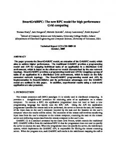
Figure 3.5: e Real Time Light Probe, an HDR video camera capturing the environment through the reflection in a mirror sphere. a): Handheld monochrome version presented in Paper I. b): In Paper IV, an RGB beam splitter was used to capture color images. c): e RTLP beam splitter solution mounted onto a trolley.

A Real Time Light Probe PΓ (x, ⃗ω ) - e ILF capture devices presented in Paper I showed that the main bottleneck was the HDR image capture, leading to the clear trade-off between capture time and ILF resolution. e mirror sphere array captured low resolution data in a very short time, and the high fidelity device captured high resolution data but required a very long time. e long capture time is a significant problem, since the entire scene needs to be kept stationary throughout the entire duration. Another area that needed improvement in both devices was the form factor; that is that capture was limited to a plane of fixed size and orientation in the scene. is motivated the development of the Real Time Light Probe, (RTLP), describe in Papers II, IV and V. e RTLP, see Figure 3.5a), is a handheld catadioptric ILF capture device that consists of an HDR video camera and a mirror sphere. e HDR video

3.1 ILF capture

27

camera was designed and implemented within a collaboration with the camera and sensor manufacturer SICK IVP AB. e current version of the camera captures images exhibiting a dynamic range of up to 10,000,000 : 1 with a resolution of 896x512 pixels at 25 frames per second, and has been implemented using the camera platform Ranger C50. In the light probe setup the maximum resolution is 512x512 pixels. e C50 camera platform is an industrial inspection and range measurement camera with a “smart image sensor”. e HDR capture algorithms are implemented as custom downloadable microcode software for this off-the-shelf camera hardware. e, 14.6 by 4.9 mm, CMOS sensor, see Forchheimer et al. [15] and Johansson et al. [27], in the camera platform has a resolution of 1536 by 512 pixels and an internal and external data bandwidth of 1 Gbit/s. Each column on the sensor has its own A/D converter and a small processing unit. e 1536 column processors working in parallel allow for real-time on-chip image processing. Exposure times can be as short as a single microsecond, and A/D conversion can be performed with 8 bit accuracy. It is also possible to A/D convert the same analogue readout twice with different gain settings for the A/D amplifier. By cooling the sensor, the SNR can be kept low enough to obtain two digital readouts from a single integration time without any significant degradation due to thermal noise. Our HDR capture methodology is similar to the multiple exposure algorithm introduced by Madden [38] and more detail is included in Section 5.1. To minimize the time disparity between different exposures we have implemented the algorithm as a continuous rolling shutter progression through the image. is means that a set of rows in a moving window on the sensor are being processed simultaneously. As soon as an exposure is finished for a particular row, the value is A/D converted and the next longer exposure is immediately started for that row, so that at any instant every row on the sensor is either being exposed or processed. All rows are not imaged simultaneously, which yields a slight “curtain” effect for rapid camera and scene motion, but, in return, all exposures for one particular row of pixels are acquired head to tail within the frame time. Two positive side effects are that almost the entire frame time is used for light integration and that the longest exposure lasts almost the entire frame time. Artifacts introduced by the time disparity between multiple exposures and rolling shutter algorithm are small, and can be compensated for in our application, as explained in Paper VI. e camera sensor in the Ranger C50 is monochrome, so color images are acquired through an externally synchronized three-camera system, one for each color channel (R, G, B). For the experiments in Paper IV, three camera units and an RGB beam splitter, see Figure 3.5b), was used to capture color images. In Papers V and VI the three cameras were equipped with red, green and blue

28

Incident Light Fields

R G B

Figure 3.6: ree cameras capturing the image of the mirror sphere from slightly different vantage points. Image registration is performed by rotation of the spherical image for each color channel.

color filters respectively, and placed at sightly different vantage points at the same distance from the center of the sphere, see Figure 3.6. Color images could then be registered by rotating the spherical image in each channel as a post processing step. Using the RTLP the plenoptic function can be sampled as a 5D function PΓ (x, ⃗ω ) by tracking its position and orientation in 3D. In Papers IV and V the camera setup was tracked using external video cameras. In these cases markers were placed on the capture rig and captured by the external cameras. e markers were then used as feature points in the tracking software, such that the position and orientation could be estimated. For the experiments in Paper VI, the RTLP was mounted onto an (x, y, z)-translation stage equipped with opto-mechanical encoders tracking the position of the light probe with submillimeter accuracy, see Figure 3.7. is setup allows for accurate capture of the plenoptic function within a 1.5x1.5x1.5 m cube. Summary and future work - Since there are no commercial cameras with the capability of capturing the extreme dynamic range needed for IBL, the development of the HDR video camera and RTLP setup has been a fundamental core component in this project. Figure 3.8 displays images from a light probe sequence captured in a scene with both indoor and outdoor illumination. On the vertical axis every 200th frame from the 1800 frame long sequence is displayed, and on the horizontal axis 6 exposures 2 f-stops apart are shown. As can be seen from the sequence the illumination varies significantly along the path. e RTLP has been successful, but there are a number of areas to improve and where more research is necessary. ere are several ways of capturing HDR video, where the use of the so called LinLog sensors currently seems to be the most promising direction. Hopefully there will soon be high resolution HDR

3.1 ILF capture

29

Figure 3.7: e RTLP mounted onto an xyz-translation for handheld capture. e position of the light probe is measured with sub-millimeter accuracy.

cameras and sensors available on the market that can be used in future capture systems. As an interesting side note it should be mentioned that Madden [38], who introduced the multiple exposure technique, stated: “e time will come when the reduced costs will make 8-bit representation the image equivalent of the black and white television”. Considering recent developments within the field of high dynamic range imaging and display technology, it seems likely that we will soon be there. We would also like to extend the capture techniques to allow for truly handheld capture. is could be achieved by the use of, existing, high precision tracking methods, such that the device can be removed from the capture rig, and maneuvered by an operator who can move freely within the scene. Such solutions include image-based methods based on the HDR image stream itself or on input from additional imaging sensors or information from other orientation sensors.

30

Incident Light Fields

Figure 3.8: Vertical axis: Every 200th frame from an HDR video sequence of 1800 frames. Horizontal axis: e frames are displayed as exposures 2 f-stops apart and tone mapped for presentation.

3.2 Rendering overview

3.2

31

Rendering overview

e main application of incident light fields in this thesis is photorealistic rendering of virtual objects placed into the scene where the ILF has been captured. is is an extension of traditional image based lighting as described by Debevec [8] and Sato et al. [58]. Given a sampling of the plenoptic function, PΓ (xk , ⃗ωk ), captured in a region Γ in space, the main objective during this process is to solve the rendering equation (Eq. 2.3) efficiently. As described in Section 2.2, this equation describes the interaction between light and matter in the scene, and omitting the self-emission term it can be formulated as: Z

B(x, ω⃗o ) =

Ωh (n)

L(x, ω⃗i )ρ(x, ⃗ωi → ⃗ωo )(⃗ωi · n)d⃗ωi

e SBRDF, ρ(x, ⃗ωi → ⃗ωo ), describes the material properties at each surface point in the scene, and is, in this setting, assumed to be known. e SBRDF associated with an object is usually a parametric function modeling the reflectance behavior, or a measurement of the reflectance properties of one or more materials. One such method for measuring the reflectance distribution of objects, in particular human faces, is described in Paper III. Here time-multiplexed illumination is used to sample the angular dimensions at each point in an actor’s face. is is performed at high speed such that the actor’s performance can be captured. e rendering equation is general enough to describe objects composed of any number of materials. Since ρ is known during rendering, the main concern is the evaluation of the integral by efficient sampling of the incident illumination, L(x, ⃗ω ). For global illumination and IBL rendering this is usually carried out using stochastic sampling methods. Here we rely on traditional rendering paradigms such as ray tracing and photon mapping, which are currently the most commonly used methods for global illumination. For clarity this overview is formulated in terms of ray tracing, first introduced by Whitted [68], of opaque surfaces, but can easily be mapped to other techniques, and can be implemented for any rendering framework supporting programmable shaders. Translucent materials and participating media can also be easily addressed by considering the integral over the entire sphere instead of the hemisphere only. e outgoing radiance, B(x, ⃗ωo ), in the direction ⃗ωo from a surface point x in the scene can be computed by solving the rendering equation. In ray tracing this is done by sampling the illumination, L(x, ⃗ωi ) incident at x by tracing ⃗ i , into the scene, and for each ray evaluating the radiance contribution rays, R from other objects and light sources observed in the ray direction. For a set of

32

Incident Light Fields

Captured Environment Camera Rc R1 X0 X1

R0

Virtual Scene

Figure 3.9: Illustration of the ray tracing process. A pixel sample in the camera corre⃗ c = xc + s · ω sponds to the ray R ⃗ c that intersects a point x0 on the object. To estimate the outgoing radiance towards the camera, B(x0 , −⃗ωc ), a number of rays randomly ⃗ 0 and R ⃗ 1 illustrate distributed over the hemisphere are used to sample L(x0 , ω ⃗ i ). R ⃗ the two cases that can occur. R0 = x0 + s · ω ⃗ 0 intersects another object at a point x1 , where B(x1 , −⃗ω0 ) is computed, again using Eq. 3.3, as an estimate of L(x0 , ω ⃗ 0 ). ⃗ 1 = x0 + s · ω R ⃗ 1 does not intersect any other object and is traced into the environment. In this case the radiance contribution L(x0 , ω ⃗ 1 ) is estimated by reconstruction of the illumination signal from the radiance sample set, Pk . e reconstruction is based on ⃗ 1. interpolation among a subset of samples in Pk that are close to the ray R

directions, ⃗ωi , where i = 1, 2, ...N , this sampling of the incident illumination function L(x, ⃗ωi ) can be described as: B(x, ⃗ωo ) ≈

N 1 X L(x, ω ⃗ i )ρ(x, ⃗ωi → ⃗ωo )(⃗ωi · n) N i=1

(3.3)

⃗ i (s) = x + s · ω where the sample rays, R ⃗ i , are distributed stochastically over ⃗ i (s), is the hemisphere. When estimating B(x, ⃗ωo ) using Eq. 3.3, each ray, R traced through the scene to evaluate the radiance contribution in the direction ⃗ωi . Since we have a measurement of the incident light field in the scene, there are two different basic cases that can occur during this tracing; either the ray intersects another surface or the ray is traced out into the captured ILF envi⃗ i (s) intersects an object, the ronment. is is illustrated in Figure 3.9. If R radiance contribution from the new surface point in the direction ⃗ωi is computed using Eq. 3.3 with a new distribution of hemispherical sample rays (case ⃗ 0 in the figure). If R ⃗ i (s) does not intersect any other object, it corresponds to R

3.2 Rendering overview y

33 y

x z

x z

a) Point

y x z

b) Line

y x z

c) Plane

d) Volume

Figure 3.10: is chapter describes rendering algorithms using ILF data where the sample region Γ is 1D linear paths b), 2D planes c) and full unrestricted point clouds sampled irregularly in 3D space d). Using traditional IBL rendering techniques temporal variations in the illumination can be captured and recreated a single point in space as a function of time, a).

⃗ 1 in Figa radiance contribution in the ILF data set. is is illustrated by ray R ⃗ ure 3.9. For R1 = x0 + s · ⃗ω1 , the radiance contribution, L(x0 , ⃗ω1 ), is estimated by reconstruction of the illumination signal from the ILF sample set, Pk . To estimate L(x0 , ⃗ω1 ) we want to identify a subset of radiance samples, Pk⋆ ⊂ Pk , in ⃗ 1 , such that the radiance contribution L(x0 , ⃗ω1 ) the neighborhood of the ray R can be reconstructed. For any light probe sequence we assume that the angular dimensions are densely sampled such that any angular variation in the environment is captured. We also assume that the angular sample region, Ωs , is the same at each spatial sample. is means that L(xk , ⃗ωi ) can be reconstructed at any given sample point, xk ∈ Γk for ω ⃗ i ∈ Ωs . It also means that the radiance contribution ⃗ i (s) = x + s · ⃗ωi , where x ∈ Γ, ⃗ωi ∈ Ωs , can be corresponding to any ray R reconstructed from Pk if the spatial sampling is dense enough to capture the frequency content in the environment. To efficiently find the neighborhood of radiance samples, Pk⋆ ⊂ Pk , for a ⃗ i , the sample set, Pk , is stored at 1D lines or 2D planes in space. is ray R might require re-projection of Pk , as described in Section 2.4. e dimensionality of the geometry, whether it is a line or a plane, depends on the spatial ⃗ i , are dimensionality of the input data. During rendering, the sample rays, R ⋆ projected to these geometries, where the neighorhood, Pk , can be efficiently determined using the Euclidean distance between points on this geometry. e following two chapters describe the process of rendering synthetic objects illuminated by sequences of HDR light probe images of different spatial dimensionality, see Figure 3.10. Section 3.3 describes techniques for rendering synthetic scenes illuminated

34

Incident Light Fields

by incident light fields constructed from light probe sequences captured along linear 1D paths in space, in the 2D plane as 180◦ field of view fish-eye images of the upward hemisphere, and as 360◦ light probe images captured in free form manner in 3D space. For completeness a set of renderings using traditional IBL techniques, but with time-varying light probe data, are also displayed and discussed in Section 3.4. For clarity, a discussion related to the impact of the sample geometry, (mirror sphere), and compensation for artifacts introduced by the particular camera setups used during capture has been left out. Such implementation details can be found in the included papers. Remark - It should be noted that, for clarity, Eq. 3.3 describes the basic idea behind the stochastic ray tracing approach for solving the rendering integral, and that there are several considerations that have to be taken into account in an actual implementation. First, the algorithm is clearly recursive, which leads to implementation issues such as what recursion depth to use, the number of ray samples at each depth, should the hemisphere be sampled in the same way at each depth etc. Secondly, for an efficient and general rendering framework care needs to be taken in choosing which rendering algorithms to use for what. Photon mapping might be the best choice in simulating some lighting effects while radiosity, ray tracing or even scan line based algorithms might be the best choice for others. ere are also several non-trivial considerations involved in implementing efficient geometry representation, spatial scene partitioning schemes, shading systems, realistic material models etc. Also of interest are the plethora of techniques for improving sampling efficiency during rendering. Such importance sampling methods, (see Section 5.2 for an overview), aim to improve the selection of sample directions based on knowledge of the functions L and ρ, such that sample variance is reduced and the solution converges to a low-noise image using a smaller number of samples.

3.3 Rendering with incident light fields

35

Captured Environment y

0

x0

z0

zn

z

zp Virtual scene xp x

Figure 3.11: For illumination captured along linear 1D paths in space the radiance contribution, L(x, ω ⃗ i ), at an object point x is found by finding the point xp along the ray closest to the principal axis of the capture, i.e. the z -axis. e closest radiance contributions in Pk can then, for the sample direction ω ⃗ i , be determined from zp .

3.3

Rendering with incident light fields

e following techniques are based on the assumption that the illumination in the scene is measured in such a way that spatial variations are captured. In the experiments conducted within the scope of this thesis this is achieved by keeping the illumination in the scene stationary for the duration of the capture, as described in Section 3.1, thus the plenoptic function is captured within a region, Γ, as: PΓ (x, ⃗ω ) = PΓ (x(t), ⃗ω (t))

is means that the captured ILF data describes the incident illumination at a set of points distributed along one or more spatial dimensions. Spatial variations 1D - Paper V describes a technique for rendering with illumination captured along linear 1D paths in space. is can be described in a coordinate system such that the principal axis of the capture region, Γ, corresponds to a segment, [z0 , zn ], along the z -axis. In this 1D case the radiance sample set, Pk , is stored as a set of dense angular measurements, light probes, at discrete positions, {zk }, along the z -axis, where z0 = min ({zk }) and zn = max ({zk }). To estimate L(x, ⃗ωi ) at each point, x, in the scene, we identify the radiance ⃗ i , as illustrated contributions in the sample set, Pk , closest to each sample ray, R

36

Incident Light Fields

Figure 3.12: An example rendering of a synthetic scene illuminated by a 1D light probe sequence. e sequence consists of around 700 HDR light probe images, and captures the high frequency spatial variation in the high contrast illumination.

in Figure 3.11. For surface points located on the z -axis, i.e. x = (0, 0, z), the closest radiance contributions for a given ray direction, ⃗ωi , in the sample set Pk can trivially be found by the Euclidean distance to points in {zk }. However, in the general case surface points, x, are not located on the z -axis. To find the ⃗ i in the scene, neighborhood of radiance contributions, Pk⋆ ∈ Pk , for any ray R ⃗ we find the point xp along the line ⃗q(s), defined by Ri , that is closest to the z -axis: ⃗q(s) = x + s · ω ⃗i ∆ =

q

⃗qx2 + ⃗qy2

xp = x + (arg min ∆) · ω⃗i s

(3.4)

Since the principal axis of the capture coincides with the z -axis, the z -component, zp , of the point xp = (xp , yp , zp ) can be used to identify the closest points in {zk }, and thereby also Pk⋆ . If zp falls outside the sample region, a clamp to edge extrapolation scheme is used to ensure a predictable behavior of the algorithm, that is if zp < z0 , zp is clamped to z0 , and similarly if zp > zn , zp is clamped to zn . e main reason for the extrapolation is that most rendered points will use lighting information from a wide range of positions along the capture path. In fact, even for simple, first-hit diffuse illumination, most points will use samples from the entire spatial extent of the data set, and be subject to extrapolation for some angles ⃗ω .

3.3 Rendering with incident light fields

Environment

37

Auxiliary geometry R1 R2 x x

R´2

R3 R´1 ILF capture area

a) Rendering with 2D ILF

b) Depth correction

⃗ i ) is estimated by projecting the corresponding ray to the ILF Figure 3.13: a): L(x, ω ⃗ 1, R ⃗ 2 and R ⃗ 3 explained in the text. b): e plane. e figure illustrates three cases R original, here central, ray is back-projected to the ILF capture plane, where the closest spatial sample positions are identified. For each sample point the depth correction recalculates the direction such that the direction vectors converge at the intersection with the auxiliary geometry. Assuming that the illumination is directionally smooth, this improves the sampling of the ILF.

Given Pk⋆ , we can reconstruct L(x, ⃗ωi ) by applying some appropriate reconstruction kernel. In Paper V, trilinear interpolation was used for the two angular coordinates and the single spatial coordinate for this reconstruction. Figure 3.12 displays an example rendering of a synthetic scene illuminated by a linear 1D light probe sequence. e sequence was captured using the RTLP, see Section 3.1, and the rendering was performed using the above algorithm, also described in Paper V. e sequence consists of around 700 HDR light probe images, and captures the high contrast spatial variations in the direct lighting and the indirect environment illumination accurately. e principal light source in the scene is a high intensity light projector, and the striped shadow pattern is created by an occluding object in the ray path. e rendering was produced using a custom plugin for Pixar’s PRMan. Spatial variations 2D - Many lighting environments can be accurately captured even if the capture is restricted to a 2D plane. e set of spatial sample points, {xk }, of the radiance contributions in the sample set, Pk , can then be described as 2D coordinates, {uk }, in the capture plane. One clear advantage of planar capture is that such a device is easier to implement compared to an apparatus

38

Incident Light Fields

that is allowed to move in 3D, especially for automatic or computer controlled measurement. One approach for capturing and rendering with 2D ILF data is presented in Paper I. In these experiments, the angular capture region, Ωs , was restricted to the hemisphere above the plane, but the rendering technique generalizes to full 360◦ HDR images. An example 2D ILF data set is displayed in Figure 3.4. When estimating L(x, ⃗ωi ) for 2D ILF data , the neighborhood, Pk⋆ ⊂ Pk , ⃗ i (s) = x + s · ω of radiance contributions for the corresponding ray R ⃗ i can ⃗ be found by back-projecting Ri to the ILF plane along the −⃗ωi direction. is back-projection is illustrated in Figure 3.13a), where the back-projected rays are ⃗ ′ i . Let also up denote the intersection point of the back-projected ray denoted R ′ ⃗ Ri and the ILF plane. Since we assume that the angular domain Ωs is densely sampled, Pk⋆ can, for the ray direction ⃗ωi , be found at the spatial sample points u⋆k = {uk : |uk − up | ≤ ϵ}, where ϵ is the radius of the spatial neighborhood. ⃗ i , can then be reconstructed from the e contribution along the sample ray, R ⋆ neighborhood, Pk , of radiance samples. Figure 3.13a) displays three cases that can occur during evaluation of L(x, ⃗ωi ). ⃗ 1 is back-projected, R ⃗ ′ , to the ILF plane, and falls inside the captured e ray R 1 area, Γ, where the illumination is reconstructed using linear interpolation between the closest radiance contributions in both the spatial and angular dimen⃗ ′ , of the sample ray R ⃗ 2 intersects the extended sions. e back-projection, R 2 ILF plane outside Γ. For sample rays that intersect the plane outside the sample region, that is at points up ∈ / Γ, a clamp to edge extrapolation strategy is used, similarly to the 1D case, such that the closest spatial measurement on the boundary of the spatial sample region is chosen as representative and used for the reconstruction. In Paper I the angular domain, Ωs , was restricted to ⃗ 3 is not represented in the data set. the hemisphere above the plane, therefore R Downward-facing directions are assumed to be “zero”, and will not contribute to the integral. In Paper I a geometric representation, called auxiliary geometry, of the scene ⃗ i , during rendering. Each sample ray, is used to intercept the sample rays, R ⃗ i , is back-projected as described above to find the neighborhood of sample R positions in the plane. To improve the sampling of the ILF, a depth correction process similar to that presented by Gortler et al. [18] is performed. Once the spatial samples in the plane are identified, the depth correction recalculates the directions such that the direction vectors converge at the intersection with the auxiliary geometry, see Figure 3.13b). e auxiliary geometry now serves as depth information for the lighting environment captured by the ILF. e closer the auxiliary geometry approximates the geometry of the lighting environment

3.3 Rendering with incident light fields

39

Figure 3.14: Example renderings using 2D ILF illumination. Compared to the traditional IBL renderings in Figure 3.1, these ILF renderings are clearly more accurate in the reproduction of the illumination in the scene, as they capture and recreate both the spatial and angular variation in the illumination. e 2D ILF data used in the renderings was captured using the computer controlled translation stage described in Section 3.1.

that ILF was captured in, the more the directional sampling will be improved. Note that the auxiliary geometry was necessary in Paper I due to the rendering software architecture. e depth correction process can also be thought of as a projection of the ILF radiance data set, Pk , onto a geometric model of the scene and, as such, can be used with any rendering framework to improve sampling. is is analogous to the re-projection of the radiance sample set, Pk , to a set of surfaces in the scene described in Section 2.4. Figure 3.14 displays two example renderings with 2D ILF illumination from the experiments in Paper I. e 2D ILF data sets used in the renderings were captured using the computer controlled translation stage setup described in Section 3.1. Each data set contained around 1, 000 HDR images of the hemisphere captured, using a 180◦ field of view fish-eye lens, in a regular grid within the planar sampling region, Γ. e renderings using ILF illumination should be compared to the traditional IBL renderings and reference photographs displayed in Figure 3.1. Although the renderings contain artifacts, as discussed below, the ILF approach clearly recreates the illumination more accurately than the traditional renderings.

40

Incident Light Fields Π0

Π4

ILF surfaces

Camera Rc

R1

R0

Π1

Π5 X

Π2

Virtual Scene

Figure 3.15: e ILF incident onto the spatial capture region, Γ, is re-projected to a set of ILF planes, Πn , enclosing the scene. At each ILF plane a 4D light field function, In (u, ω ⃗ ), with 2D spatial extent describes the spatial and angular variation in the illumination incident onto the scene. During rendering L(x, ω ⃗ i ) can be efficiently estimated by sampling the ILF planes.

e renderings in Figure 3.14 contain artifacts from two main sources. First, the spatial sampling density is not high enough to recreate the illumination without block-like artifacts. In Paper I the spatial resolution was limited by the capture. However, the RTLP, see Section 3.1, addresses this problem by allowing capture at 25 frames per second, which is more than two orders of magnitude faster than the approach used in Paper I, and makes it practical to capture ILFs with much higher spatial resolution. Secondly, especially the right image contains noise from the rendering process. is is due to the fact that the rendering software did not support importance sampling of the ILF, and that the sampling therefore was performed in a blind stochastic fashion. e renderings in Figure 3.14 were produced using the RADIANCE lighting simulation and rendering system [67], which was not equipped with the necessary mechanisms for importance sampling of the ILF light sources. In the experiments in Paper I the spatial sample points where distributed in a regular grid. is is, however, by no means necessary and extensions using irregular spatial sampling or adaptive sampling techniques are straightforward to implement. e main difference from the approach described above is the implementation of efficient random access of the radiance contributions in the data set during rendering.

3.3 Rendering with incident light fields

41

Π0

ω2

ω1 Π1

ω3

Π2

Sample region

Figure 3.16: e radiance samples are sorted into angular buckets based on the angular quantization imposed by the light probe images. Each angular bucket contains a parallel projection of the sample region, Γ. Different incident directions, illustrated by ω ⃗ 1, ω ⃗ 2 and ω ⃗ 3 , are re-projected to different areas in the ILF planes Πn .

Spatial variations 3D - Paper VI describes a technique for capturing the plenoptic function in 3D space and algorithms and data structures for rendering synthetic scenes illuminated by such ILF data. Here the environment is captured using the RTLP, described in Section 3.1, and a mirror sphere setup, such that the angular sample region, Ωs , captured by each HDR image in the sequences is close to 360◦ . In the presented technique, the capture path is traced by manual motion in a free-form manner, allowing for operator-directed variations in sampling density to reflect regions of particular interest in the scene. e irregular spatial sampling is not resampled to a regular grid but, instead, maintained in its original non-uniform distribution. is reduces reconstruction errors, and makes it more straightforward to perform adaptive sampling and data decimation. An example of such decimation is described in Paper VI. Given a sampling of the plenoptic function captured in 3D space the set of corresponding radiance samples, Pk , are re-projected to a set of 2D surfaces, Πn , enclosing the scene, where n = 1, 2, ..., N . is re-projection process is illustrated in Figure 3.15 and further described in Section 2.4. At each ILF surface, Πn , a subset of the radiance samples, PkΠn ⊂ Pk , describes the light field, In (u, ⃗ω ) incident onto the sample region, Γ, as a 4D function of two spatial coordinates, u = (u, v), in the plane and the angular direction, ⃗ω . e effect of the re-projection of the radiance sample set is a reordering of the samples such that the spatial sample points, xk , in 3D space can

42

Incident Light Fields

a) Angular buckets in top plane

θ

d) Sample rays in delaunay triangulation

v

φ b) Angular buckets close-up

u c) Spatial variation

Figure 3.17: e ILF data structure. a): e radiance samples PkΠn are, at each ILF plane, Πn , sorted and binned on their angle. Each angular bucket stores a parallel projection of the sample region. Here this is illustrated by the mean radiance value in each bucket in a plane above the sample region. b): shows the spatial variation within each bucket in an angular region in the ILF plane. c): displays the reconstructed illumination signal in one angular bucket. d): For fast random access, a Delaunay triangulation is computed on the individual sample positions in each angular bucket, and the triangles are stored in a balanced kd-tree structure.

be described as 2D coordinates, ukΠn , on the ILF surfaces, Πn . After the re-projection of the radiance data set, Pk , to the ILF planes, Πn , the radiance contributions, PkΠn , associated with each plane are sorted on their angle. e reason for this angular binning is that the angular domain, Ωs , is quantized to the light probe resolution and that the spatial sample points, ukΠn , are non-uniformly distributed. e angular binning is illustrated in Figure 3.16. In the setup in Paper VI, the camera orientation is kept fixed during capture and, therefore, the same set of angles will be captured by each light

3.3 Rendering with incident light fields

43 u2

u1 u

ω1

ω4

ω2 ω

ω3 ω

ω x

u3

u4

x

Figure 3.18: ILF ray sampling. e value at sample position u in direction ω ⃗ is adjusted by projection along the four nearest sampled directions in the angular domain, followed by interpolation in the spatial domain.

probe image. For unrestricted capture where the orientation is allowed to vary, the light probe images can be re-sampled to a common coordinate system to maintain the regular angular sampling. e angular binning presents a data structure, illustrated in Figure 3.17, that allows for fast random access of radiance samples during rendering, since two of the four dimensions can be indexed using the direction, ⃗ωi , of the sam⃗ i . Within each angular bucket the irregular point cloud of spatial ple ray, R sample points describes a parallel projection of the sample region, Γ. To allow for fast access of the closest spatial sample points to any given intersection ⃗ i , and the ILF planes, Πn , a Depoint, u, between rendering sample rays, R launay triangulation is computed within each bucket. For efficient lookup a balanced kd-tree structure is used to index the triangles. In Paper VI barycentric interpolation between sample points, ukΠn , in the Delaunay triangulation is used to reconstruct the illumination signal at any point in the plane for a given direction. In order to solve the rendering equation, Eq. 2.3, the illumination distribution L(x, ⃗ωi ) at each point x in the scene is computed by estimating the radiance contributions arriving at the point x from each ILF plane, Πn . In ray tracing this is performed by, at each scene point x, tracing the sample rays, ⃗ i (s) = x + s · ω R ⃗ i , towards the ILF planes. e reconstruction of the radiance contribution, L(x, ⃗ωi ), is performed by first identifying the neighborhood, ⃗ i at the intersection Pk⋆Πn ⊂ PkΠn , of radiance contributions for the sample ray R ⃗ i and the ILF plane Πn . is is illustrated in Figure 3.15, where point, u, of R ⃗ ⃗ 1 , are traced from the point x and intersect the ILF planes two rays, R0 and R

44

Incident Light Fields

Figure 3.19: A synthetic scene rendered using ILF illumination captured in 3D. e illumination in the scene is created by two principal light sources, an area light with a perforated planar blocker and a projector light with a filter gobo creating the four squares. is rendering should be compared to the corresponding traditional IBL rendering and the reference photograph in the bottom row in Figure 3.1.

Π4 and Π0 respectively.

By assuming that the angular domain is densely sampled and denoting the 2D spatial sample points of the ILF radiance samples, PkΠn , by ukΠn , the neighborhood of radiance contributions, Pk⋆Πn , can for the sample ray direction, ⃗ωi , be found at the set of ILF sample points given by {ukΠn : |ukΠn + u| ≤ ϵ}, that is, all spatial points within a neighborhood with radius ϵ. L(x, ⃗ωi ) can now be reconstructed from the radiance contributions in Pk⋆Πn . In Paper VI, the interdependency of u and ⃗ω is handled similarly to the ⃗ i = x + s · ⃗ωi , has an depth correction method used in Paper I. A sample ray, R actual hit point, u, on the ILF plane, but typically neither the exact direction ⃗ωi nor the exact point u have been sampled directly, hence interpolation is required in both the angular and spatial dimensions. is 4D interpolation is performed in two 2D steps. First, the four closest angular samples, ⃗ω1...4 , are picked and four rays are projected from the scene point, x, in those directions to four adjusted hit points, u1...4 . e radiance contributions at those points are then evaluated by the previously described barycentric interpolation in the Delaunay triangulated set of points, and the final value is computed by bilinear interpolation between those four points. is ray sampling is illustrated in Figure 3.18. e sample volume, Γ, typically does not cover the entire scene, but a smaller region of special interest where highly detailed rendering is desired.

3.3 Rendering with incident light fields Area light source

45 Projector spotlight

Blocker White surface

Figure 3.20: An overview of the test scene setup in which the ILF data was captured for the rendering in Figure 3.19. e scene contains one large area light source with a perforated occluding blocker and a projector light source with a filter gobo creating the four differently colored squares.

For points x ∈ / Γ, data is available only for directions, ⃗ω , that intersect Γ. To enable rendering of objects outside Γ, extrapolation is employed. For directions not intersecting Γ, a clamp-to-edge extrapolation finds the closest point on the boundary and assumes it is representative for all x ∈ / Γ in that direction. is assumption removes the spatial variations outside Γ, but maintains a variation with direction to the sample volume and gives a predictable behavior even outside the sampled region. Support for ILF illumination can be implemented in any standard global illumination framework which evaluates light contributions along explicit sample rays. Figures 3.19 and 3.21 display two example renderings where the described technique for use of ILF illumination captured in 3D was used. e renderings were produced using a custom plug-in for mental ray from mental images. e illumination in Figure 3.19 is created by an area light in the ceiling and a light projector creating a high frequency spatial pattern, four colored rectangles. e effect of the area light can be seen in the reflection in the toy cars. e area light is occluded by a perforated plane creating the pattern seen in the reflections. As can be seen, the high frequency spatial pattern created by the projector light was sampled densely enough to be recreated properly. is rendering should be compared to the traditional IBL rendering of the same scene using only a single omni-directional illumination measurement displayed in the bottom row of Figure 3.1. An illustration of the real world test scene setup in which the ILF illumination used in Figure 3.19 was captured can be seen in Figure 3.20. Figure 3.21 displays a scene with three synthetic objects rendered using illu-

46

Incident Light Fields

Figure 3.21: ree synthetic objects on a real table in a real scene.e illumination for this rendering was captured in a castle in Linko¨ping, Sweden, and is based on a sequence of more than 40, 000 light probe images. Each point, x, in the rendered scene has its own individual HDR environment map reconstructed from the ILF data.

mination captured in a castle in Linko¨ping, Sweden. e captured HDR image sequence consists of more than 40, 000 light probe images, or more than 9 billion radiance samples. e sample rays were re-projected to twelve different ILF planes, displayed in Figure 2.1b), where six of the planes each contained the radiance contribution from a high intensity and high contrast region in the environment with a large impact on the rendering integral. e high intensity regions were extracted from the captured ILF data as described in Section 3.6. e six remaining planes represent the low intensity and low contrast background illumination. Note that each scene point, x, in the rendered scene has its own individual HDR environment map reconstructed from the ILF data, that is parallax in the captured environment is preserved. Paper III describes a technique for measuring the reflectance properties, ρ(x, ⃗ωi → ⃗ωo ), of performing actors. is is performed using a light stage setup as introduced by Debevec et al. [10], see also Section 5.3 for an overview of the technique. Light stage data sets are often rendered using traditional IBL tech-

3.3 Rendering with incident light fields

47

niques using a single light probe image, La (⃗ωi ), as illumination. Since both the illumination distribution and SBRDF are based on real world measurements this achieves high levels of realism. Based on photometric stereo algorithms, see Woodham [70], Paper III also describes a method for extracting surface and material parameters. Under the assumption that the captured faces exhibit a diffuse component in the reflectance properties, photometric stereo is used to estimate a surface normal and diffuse albedo at each captured point in subject’s face. Using the extracted parameters, the paper also describes how stylized images of the captured subject can be rendered based on the extracted parameters. In this context, that is incident light field illumination, we are interested in rendering such captured performances as illuminated by spatially varying illumination. Initial work in this area was conducted by Masselus et al. [43]. ey captured 6D reflectance fields by varying both the position and direction of the incident illumination in the sampling of the reflectance functions. ey also demonstrated how such 6D reflectance fields could be rendered and illuminated by 4D incident light fields. e light stage apparatus developed for Paper III only sampled the angular dimensions of the reflection function at each captured point, that is a locally 2D reflectance field. In order to use 4D ILF data as illumination we need to know how the reflectance function varies with both direction and position of the incident illumination. is can also be realized by estimating the position at which each reflectance function has been captured, that is combining the reflectance field with a geometric model of the captured subject. Jones et al. [28] describes a method for rendering captured reflectance fields as illuminated by simulated 4D incident light fields by employing the same capture and parameter extraction method as described in Paper III, but also capturing the geometry of the face by projecting structured light patterns onto the actor’s face during the reflectance capture. Using such data, we can use the extracted geometry and reflectance parameters to render captured faces as illuminated by the 4D ILF data captured in real world scenes. Figure 3.22 displays a series of renderings using the extracted normal directions, diffuse albedo and estimated geometry of the actor’s face. e left column displays the estimated normal directions at each point in the face, the middle column displays the estimated diffuse albedo, and the right column displays renderings of the actor illuminated by a captured light ILF. e reflectance data and geometry used is an excerpt from a captured sequence of a performance. e images were rendered using an in-house deferred shading software developed for interactive rendering of scenes illuminated by captured ILFs. e system does not support global illumination, and therefore only first order illumination effects are simulated. However, Jones et al. [28] suggests a

48

Incident Light Fields

Figure 3.22: Left: estimated normals. Middle: estimated diffuse albedo. Right: renderings using the captured geometry and reflectance parameters to allow for rendering with spatially varying illumination captured using the techniques described in this thesis.

straightforward extension to include also higher order lighting global illumination effects. Summary and future work - is chapter describes a set of techniques for rendering synthetic objects as illuminated by spatially varying illumination captured using the ILF capture techniques described in Chapter 3.1. e described methods assume that the scene is stationary during capture, and allows for ren-

3.3 Rendering with incident light fields

49

dering using illumination varying along one to three spatial dimensions. For efficient rendering the techniques rely on projection of the captured data set, Pk , to surfaces or lines in the scene, where the closest radiance contributions to any given sample ray during rendering can be found efficiently. e described rendering techniques are straightforward to implement in any global illumination software that supports programmable light source shaders, and that performs rendering by evaluating radiance contributions along rays defined by a position and a direction. Future directions include real time rendering of synthetic objects illuminated by 4D incident light fields. is is important both in real time applications such as computer games and augmented reality, and also for fast preview rendering in the viewport of modeling software to aid digital artists and animators in the modeling and setup of virtual scenes.

50

Incident Light Fields

Figure 3.23: A set of example renderings from an animated sequence where a single light probe image is used as illumination for each frame. To the left of each rendered image, the corresponding HDR light probe image is displayed.

3.4

Rendering with light probe sequences

Temporal variations - Perhaps the most straightforward way to use HDR light probe sequences as illumination in renderings is to use traditional IBL methods, as introduced by Debevec [8]. In this case only one light probe image is used for each rendered frame. In this way temporal variations in the illumination can be captured. Since the traditional rendering technique is used, this is supported in most modern rendering software. In this case only the angular variation in the illumination is considered in each rendered frame, but as a function of time. e factor for incident illumination in the rendering equation is then described as L(⃗ωi , t). e position of the capture device can be varied such that the illumination is captured along a path in the scene, but the 2D approximation is assumed to hold. is means that the spherical time-varying illumination distribution L(⃗ωi , t) can be reconstructed from: PΓ (x(t), ⃗ω (t), t)

i.e. the light probe image captured at time t. PΓ (x(t), ⃗ω (t), t) is captured

3.4 Rendering with light probe sequences

51

at position x(t) in the scene, and therefore allows for rendering objects as they would appear if they were traveling along the curve x(t). Since only one light probe image is used in each rendered frame, the traditional IBL rendering algorithms, as described by Debevec [8], can be employed. Figures 3.23 displays a series of renderings, where the illumination was captured as sequence over time, PΓ (x(t), ⃗ω (t), t). Each rendered image uses only one light probe image, displayed to the left of each rendering, as illumination. is technique cannot recreate any spatial variations in the illumination. For environments exhibiting strong spatial variation, flickering artifacts can be observed. is is due to the fact that the illumination for the entire scene is approximated by one spherical distribution L(⃗ωi , t), and strong light sources visible in one light probe might disappear in the next. However the technique is useful for environments where the spatial variations are slow compared to the size of the synthetic scene. Summary and future work - Rendering with light probe sequences in dynamic scenes is not the main focus of this thesis, but is nevertheless an interesting area to investigate. It is included here mainly for completeness. e technique could be useful in many situations, where elaborate capture of the full dimensionality of the plenoptic function is difficult or impossible due to time or other constraints. Initial work towards importance sampling and other techniques for speeding up rendering time, taking into account temporal coherence between frames in the HDR sequence, was performed by Havran et al. [21, 22] and Ghosh et al. [16]. Unfortunately, captured sequences of HDR light probe images are still rare, and the existing ones, apart from ours, are either captured as time lapse sequences over an extended period, of low quality or simulated. Future work in this area includes efficient representations, compression of capture sequences and building a library of HDR light probe sequences for others to use in future research.

52

3.5

Incident Light Fields

Illumination interaction and visualization

An ILF describes the illumination within a volume in space by a potentially very large set of radiance samples, Pk . During ILF data processing and analysis it is very useful to be able to visually inspect the illumination in the captured scene and to interact with the data. e techniques described here are developed for three main purposes: visualization of captured scenes, placement of ILF surfaces for the ray re-projection, and selection of small subsets of radiance samples in the captured radiance data set, Pk , corresponding to scene features such as light sources and other high energy regions. Visualization of the scene illumination and protocols for intuitive interaction with the radiance data set are not trivial problems. e size of the captured data set, Pk , is usually very large, in the order of tens of GB or more. is chapter describes the visualization and interaction techniques used for placing the ILF surfaces for the re-projection of captured scenes described in Section 2.4, and in the extraction and editing of high energy regions, illuminants, in the scene described in Sections 3.6 and 3.7. e following discussion assumes that the ILF has been captured similarly to the technique described in Paper VI, i.e. as a set of light probe images non-uniformly distributed in 3D. Volume visualization of local properties - As described in Paper VI the captured radiance data set, Pk = P (xk , ⃗ωk ), is a 5D function. e, in most cases, very large data size and 5D nature of this function makes it difficult to visualize and analyze directly. Instead we take another approach, where the captured radiance samples, Pk , are back projected to a volumetric data set defined over a regular grid in a volume in space. For each grid cell located at a posi˜ xi ), suitable for visualization are computed using tion, xi , local properties, Q( a reconstruction kernel, gQ . is back-projection, described in more detail in Section 2.5, is possible since the sample region, Γ, is assumed to be free from internal occlusion. e main objective in this stage is to supply an intuitive interface for visualizing a captured data set, and to allow for placement of ILF surfaces in the scene. After placement these surfaces are subject to the radiance re-projection process described in Section 2.4, where each radiance sample in the data set, Pk , is associated with an ILF plane, Πn , to create a corresponding ILF function, In (u, ⃗ω ). Using the back-projection method described in Section 2.5 a variety of local ˜ , can be estimated at each grid point, xi . e local properties are properties, Q visualized by either direct volume rendering with transfer functions or by slicing of the volume. e slicing technique allows the user to place arbitrarily

3.5 Illumination interaction and visualization

53

Figure 3.24: Visualization of the partial density for radiation reconstructed by back projection of the captured radiance data set, Pk , from the sample region, Γ, to a regular grid within a volume P ′ with 512 x 256 x 512 voxels. Top and middle show two different exposures (left and right) of the room seen from two different view points. Note how the captured radiance samples are visible as streaks from the capture region, Γ, in the ILF box placed around the light source in the ceiling. Bottom displays a closeup of three chairs brought into focus by the placed ILF boxes. e red box displays the approximate extent of the capture region, Γ.

54

Incident Light Fields

Figure 3.25: A sequence of different slices in the volume. e group of chairs is revealed by placing a slice at the position where they are in focus.

oriented boxes and planes within the volume, where each point on a cutting plane shows the intersected voxels. e direct volume visualization is generally most useful for displaying and finding regions of convergence for high intensity radiance samples corresponding to light sources in the scene, and the slicing is most useful for visualizing the captured scene from the inside. An example visualization using the slicing technique is displayed in Figure 3.24. Here the partial density of radiation, E ′ , is displayed at two different exposures. In this case the mean intensity for the three spectral bands is used, but using all three color channels is also possible. ere are a number of ILF boxes placed within the volume, one constituting the walls of the room, one corresponding to a chandelier in the ceiling and three around a set of chairs in the scene. e red box in the upper left image displays the approximate extent of the capture region, Γ, from which the radiance samples are back-projected. is ILF data set, captured in a castle in Linko¨ping, is also used in the rendering in Figure 3.21 in Section 3.3. e captured radiance samples can be thought of as a large synthetic aperture captured in 3D. At voxel positions, xi , located at unoccluded surface points, x, in the scene, the scalar value will correspond to the reflected or emitted radiance, B(x, ⃗ωo ), from that point, x, integrated over the solid angle, ΩΓ (xi ), subtended by the capture region, Γ. e position of an object can therefore be found by moving the slice plane within the volume such that the

3.5 Illumination interaction and visualization

55

Figure 3.26: is image displays the partial density of radiation (left column), the variance in the radiance contribution within each voxel (middle column), gradients (right column), for two different positions of the wall ILF plane. It should be noted that this is an interactive tool, and does not lend it self very well to this still image presentation.

object exhibits maximum focus, as displayed in Figure 3.25. e degree of accuracy of this technique is dependent on the relative occlusion between objects in the scene, but is often useful for finding important features such as light sources or other high intensity regions. Figure 3.26 also displays slices from the volume, but in this case one of the walls is moved towards the observer. Apart from the partial density of radiation, E ′ , (left column) this image also displays two other local properties: the variance in radiance value within each voxel (middle column), and the gradient magnitude of E ′ (right column). ese are cues that can assist the user to find regions of focus for certain objects, and to explore the captured data set. Direct volume rendering is useful for visualizing direct light sources and other high intensity regions. Figure 3.27 displays two renderings produced using ray casting of the partial density of radiation volume. In 3.27a) the transfer function is set to display only high intensity regions. Here it is clearly evident that the chandelier in the ceiling, the windows, a mirror on the right wall and a small spotlight located at the convergence point close to the capture region on the right hand side are the main contributors of illumination in the scene. In 3.27b) the transfer function is set to display only low intensity voxels. In this case the curtains around each window are clearly visible and by using cut

56

Incident Light Fields

a) High intensity voxels

b) Low intensity voxels

Figure 3.27: Direct volume visualization of the partial density of radiation, E ′ , using ray casting. a) is rendered using a transfer function that displays only high intensity radiance samples. b) is rendered such that only low intensity samples are visualized. Note that the two images are rendered from slightly different vantage points.

planes in the volume other features can be investigated. Note also that this image contains holes in the data where the high intensity regions are located. With the help of the described visualizations, the user can place planes and boxes within the volume. ese surfaces are then used for re-projection of the radiance data set, Pk . ese techniques are useful in the extraction and editing of illuminants as described in Sections 3.6 and 3.7. It is also useful to further analyze the re-projected radiance samples using the techniques described below. Light field rendering - Given a set of ILF planes, Πn , with associated 4D ILF functions, In (u, ⃗ω ), novel images can be generated within the sampling volume. is is similar to light field rendering, as described in Levoy and Hanrahan [37]. e difference in this case is that, instead of imaging small scenes captured as a 4D light field, the radiance sample set describes a very large omni-directional synthetic aperture captured in 3D such that novel images of the environment can be reconstructed within the region, Γ. e resolution of these reconstructed images is limited by the spatial sample density in Γ and the angular resolution at each point. is rendering technique is similar to that presented in Section 3.3 but, instead of estimating the incident illumination at all surface points in the scene, an image is reconstructed. is technique is useful for displaying the captured scene, but interaction with the radiance sample set, Pk , is difficult. Interaction with the 4D radiance

3.5 Illumination interaction and visualization

a) Mean radiance visualization

57

b) Maximum radiance visualization

500

0

-1000

-500

0

500

1000

1500

c) Selected subset of radiance samples corresponding to the light surces

Figure 3.28: a) Mean intensity within an angular selection corresponding to the two light sources, and b) maximum intensity for each angular bucket of one ILF plane. c) resholded radiance samples corresponding to the two light sources. In this case there is an overlap in the angular buckets, i.e. the two light sources are simultaneously visible in a number of buckets. To discriminate between the two objects the selected radiance samples are projected to a plane where they separate. Here, samples from the partly blocked area light are to the left and samples from the light projector to the right. Units are in millimeters.

sample set, Pk , is difficult since only 2D images are generated, which means that selection in the underlying 4D space is non-intuitive. e data sizes of the ILF planes are also often very large, which leads to difficulties in displaying the entire data set simultaneously on current hardware without extensive prior decimation or compression. is means that this visualization is usually performed on one or a few ILF planes, Πn , at a time. Angular bucket visualization - In Paper VI the radiance samples, PkΠn , associated with each ILF plane Πn are sorted on their angle and binned into angular buckets. is means that each bucket describes a parallel projection of the sample region. is data structure is described in Section 3.3 in the discussion on spatial variations in 3D and visualized in Figure 3.17. For each direction, ω ⃗ k , the corresponding bucket consists of a set of spatial sample points, {ukΠn }, projected to the ILF plane Πn . is means that each angular bucket describes

58

Incident Light Fields

a parallel projection of the sample region, Γ. A useful technique, described in Paper VI, for aiding the selection of subsets of radiance samples corresponding to high intensity regions such as light sources from the sample set, Pk , is to separate the angular and spatial dimensions and first make selections among the angular buckets and then selections among the spatial sample points within the buckets in the angular selection. is can also be combined with thresholding operations in order to select radiance samples within a certain intensity range. For light sources this is straightforward since they clearly stand out from the background in the HDR data. Figure 3.28 displays a visualization of: 3.28a) the mean radiance value, and 3.28b) the maximum radiance value within each angular bucket in an ILF plane. Figure 3.28a) also displays a selection of angular buckets corresponding to two light sources, an area light source in the ceiling and a projector spotlight. Figure 3.28c) displays the selected radiance samples after a thresholding operation such that only high intensity samples are selected. e selected radiance samples in Figure 3.28c) are projected, see below, to a plane where they clearly separate in the spatial domain. e visualized ILF plane is the top plane generated from the illumination data captured in the scene described in Figure 3.20 in Section 3.3. In order to discriminate between sample clusters that belong to different light sources but are visible in the same angular buckets, the radiance samples are projected to a plane that can be moved in the direction of its normal, see Figure 3.29. In this way the projection of the captured radiance samples can be investigated. Objects that are separate in the scene, will, as the plane moves, be separated in the projection to the plane and can be discriminated in the spatial domain. is allows for unambiguous selection of the clusters corresponding to different objects. Another example where this technique is utilized is described in the discussion on illuminant extraction in Section 3.6. Summary and future work - is chapter presents techniques for visualizing and interacting with the captured data sets. is is performed in different ways, but with the same goals. e main objective is to place ILF surfaces in the scene, which are suitable for representing the illumination, and to allow for selection of subsets of radiance samples in the 4D ILF space such that scene features can be extracted and edited. To visually investigate the captured scene local properties reconstructed by back projection are visualized. In this interface the user can place geometries and control the projection of radiance samples to these surfaces. Another useful technique, used in Paper VI, is to visualize the content of angular buckets that

3.5 Illumination interaction and visualization

Area light source

59

Projector spotlight Blocker

Projection plane

White surface

a) The radiance samples are projected to a plane of variable position

b) Objects separated in the scene separate in the projection

Figure 3.29: a) Unambiguous discrimination of clusters of radiance samples can be performed by projection of the, possibly thresholded, radiance samples selected in the angular bucket selection to a plane with a variable position. b) Clusters of radiance samples corresponding to objects that are separate in the scene will, as the plane moves, be separated in the projection to the plane and so can be discriminated in the spatial domain.

60

Incident Light Fields

describe parallel projections of the capture region, Γ. Individual radiance samples can, in this way, be selected, extracted and projected to new ILF planes using straightforward image manipulation techniques. It is also possible to visualize the captured scene using more traditional light field rendering techniques. As future work we would like to extend the framework and allow for more complex capture regions, not necessarily convex and compact in 3D. We would also like to apply methods similar to synthetic imaging techniques for more complex editing and selection of scene features. Manual interaction is a very important component in this process since it is very difficult to know a priori what features, except light sources, that are important for a certain scene and for a certain application. erefore it is of interest to supply the user with a set of automatic extraction algorithms that also allow for manual editing and adjustments of the data, especially for the illumination editing described in Section 3.7.

3.6 Illuminant extraction

3.6

61

Illuminant extraction

A major concern during rendering of synthetic scenes is the sampling of the radiance distribution, described by L(x, ⃗ωi ), incident at the scene point x. e main difficulty in the sampling is the potentially very high contrast between direct illumination from light sources and indirect illumination, where the indirect illumination refers to light that has undergone one or more reflections or refractions at other surfaces in the scene before arriving at the point x. Using stochastic rendering methods there is a trade-off between rendering time and image noise. In terms of ray tracing, see Chapter 3.2, we want the estimation of L at each scene point, x, to converge using as few ray samples as possible. Separation of direct and indirect illumination - Part of the sampling problem resides in that the rendering equation as presented in Eq 2.3 does not contain any information about the scene geometry. is means that the hemispherical domain, Ωh (n), at each scene point, x, has to be sampled very densely in order to make sure that both high intensity regions, (light sources), and the background are sampled sufficiently. A common method that allows for improved sampling strategies used in virtually all modern rendering software is to divide L(x, ⃗ωi ) into two parts: L = Ld + Li

where Ld is the direct illumination from light sources in the scene, and Li is the indirect illumination. e discussion below on the separation of the incident illumination and the area formulation of the rendering equation is described in detail in standard books on global illumination, see for instance Dutre et al. [12] for a nice overview, but is briefly covered here for the convenience of the reader unfamiliar to this idea. is separation of the incident illumination into two terms means that the direct and indirect illumination can be sampled separately. e observed radiance, Bi (x, ⃗ωo ) from a scene point x in the direction ⃗ωo is now described as the sum of the self-emission and two integrals, one for the direct illumination, Bd (x, ⃗ωo ), and one for the indirect illumination, Bi (x, ⃗ωo ): B(x, ⃗ωo ) = Le (x, ⃗ωi ) + Bd (x, ⃗ωo ) + Bi (x, ⃗ωo )

e radiance Bd , describing the effect of the direct illumination can now, for convenience, be described using an area formulation of the rendering equation: Z

Bd (x, ⃗ωo ) =

A

Le (y, −ω⃗i )ρ(x, ⃗ωi → ⃗ωo )V (x, y)(⃗ωi · n)

(−⃗ωi · ny ) dAn |x − y|2

(3.5)

62

Incident Light Fields

over the surface area, Ai , of the light sources in the that is as an integral S scene, where A = An , y is a point on a light source, V (x, y) is a visibility function that is 1 if x and y are mutually visible and 0 otherwise, and ny is the surface normal at the light source point y. Using Eq. 3.5 for the direct illumination, the rendering equation can now be formulated as: Bd (x, ⃗ωo ) = Le (x, ⃗ωo ) + Z

+ Z

+

A

Le (y, −ω⃗i )ρ(x, ⃗ωi → ⃗ωo )V (x, y)(⃗ωi · n)

Ωh (n)

L(x, ω⃗i )ρ(x, ⃗ωi → ⃗ωo )(⃗ωi · n)d⃗ωi

(−⃗ωi · ny ) dAn + |x − y|2

(3.6)

is means that the direct illumination can be explicitly sampled using the area formulation, while the indirect illumination can be sampled using the hemisphere representation. In virtual scenes with virtual light sources this is realized by supplying geometric representations of both the light sources and the objects in the scene. ILF illuminant extraction - An ILF can describe arbitrarily complex lighting in a scene. However, since it represents the illumination in a scene as a very large set of radiance samples, Pk , with no information about scene geometry it also presents a considerable sampling problem. Similarly to the example above, the main difficulty is the extreme contrast between direct and indirect illumination. In traditional IBL there are methods for approximating single light probe images with a set of light sources, and thereby supplying a geometric representation of the illumination to the renderer, described by Kollig and Keller [32]. Importance sampling of a single 2D light probe, described by Agarwal et al. [2] and Ostromoukhov et al. [53, 52], in traditional IBL is also straightforward but, for the 4D ILFs it is difficult to predetermine good sampling distributions for all possible case, since the important high intensity regions in the environment might differ significantly between points in the scene. Instead, motivated by the separation of direct and indirect illumination described in Eq. 3.6, we take a scene based approach and separate the high energy regions in the captured scene from the original ILF data set into Source Light Fields, (SLF), each represented at their own, individual, SLF surface. is means that the captured illumination is separated into a set of high intensity and possibly high contrast SLFs and a residual, indirect, background ILF component. In terms of Eq. 3.6 this means that the SLFs constitute the direct lighting, Ld , and, the residual ILFs the indirect lighting, Li . It should be noted that there is no formal distinction in the representation of an ILF and an SLF. e

3.6 Illuminant extraction

63

conceptual difference between the two is that an SLF should be thought of as direct illumination and an ILF as indirect illumination at each point, x, in the scene. By matching the SLF geometry to that of the high intensity areas in the scene, compact high energy clusters can be located in 3D space, and sampling can be efficiently concentrated during rendering by explicit sampling of these clusters. is representation is similar to the near field representations used in Heidrich et al. [23] and Goesele et al. [17], but in this case it is generated from illumination captured at the region of interest in the scene, not at the light sources. In this work the extraction of illuminants is performed as a semi-manual process, and was presented in Paper VI. In order to create an SLF representation of a light source or other high intensity region in a scene, the visualization and selection methods described in Section 3.5 are utilized. Both the volume visualization and angular bucket visualization techniques are useful for this task. e extraction process works as follows: first a subset of radiance samples, Pml ⊂ Pk , corresponding to a light source, l, is selected e selected radiance samples are then projected to an SLF plane, Πl , where the samples, Pml , now can be described by their intersection point, u˜ ml , with the plane, Πl , and their directions, ⃗ωml , respectively. During rendering it is desirable to have as compact a geometric representation of the SLF as possible. e position of the SLF plane, Πl , is therefore found by an optimization process such that the spatial cluster size of the projected radiance contributions determined by u˜ ml is minimized. is assumes that the spatial sample region, Γ, is larger than the illuminant, otherwise the radiance contributions will not converge. It is also straightforward to perform this process using manual inspection of the projected radiance samples. In Paper VI the optimization for the illuminant position is performed such that the SLF plane, Πl , is allowed to move with a variable offset, z , along its normal direction, and the optimal position, zl , along the plane normal is found by minimizing the projected spatial cluster size: zl = arg min (A(˜ uml (z)) z

(3.7)

where A(˜uml (z)) is a suitable measure of the cluster size of u˜ ml (z), for example the norm of its vector standard deviation, and u˜ ml (z) is the projection of uml along ⃗ωml to the plane Πl at offset zl . is results in a spatially compact representation of the SLF which is desirable in the illumination sampling during rendering. At the optimal z = zl , the convex hull, Kl , of u˜ ml (zl ) is used as an estimation of the spatial extent of illuminant l. All radiance contributions from

64

Incident Light Fields

Residual ILF planes Π2...n

Π1

Π0

Figure 3.30: Illustration of two extracted light sources. e radiance samples corresponding to each light source have been extracted and projected to two SLF planes, Π0 and Π1 , where Π0 corresponds to the projector light and Π1 to the partially occluded area light source in the ceiling. e residual, low intensity and low contrast, background illumination information is now stored at the ILF planes denoted by Π2...n . e radiance measurements are thus stored as near field representations that describe the spatial and angular radiance distribution for the emission from each light source by a 4D function.

the original sample set, Pk , that intersect Kl are then stored in the SLF to describe both the shape and detailed appearance of the illuminant. e radiance contributions, Pml , associated to the extracted SLF are removed from the residual background ILF during this process, and the holes are filled by interpolation. Both localized point-like light sources and area light sources can thus be extracted to SLF planes with optimal position and spatial extents, closely representing actual illuminants. Figure 3.30 illustrates the extraction and re-projection of the two illuminants in the example scene illustrated in Figure 3.20 in Section 3.3, and also used for the rendering of the toy cars in Figure 3.19. e two illuminants, one projector spotlight and one partially occluded area light source are, in Figure 3.30, extracted to the SLF planes denoted Π0 and Π1 , where the spatial and angular distribution of the light sources are stored as a 4D function. e extracted radiance contributions are removed from the residual background ILF data represented as Π2...n in Figure 3.30. In essence, this procedure performs a 4D clustering of the measured radiance contributions in the scene such that high intensity regions can be sampled efficiently during rendering. Figure 3.31 displays two example renderings to demonstrate the improved rendering efficiency enabled by the illuminant extraction. In 3.31a) a rendering without illuminant extraction is displayed, the illumination in the scene

3.6 Illuminant extraction

65

a) Brute force, ILF only, rendering, five hours

b) Rendering with extracted lilluminants, 4 minutes

Figure 3.31: a): An example rendering without illuminant extraction. e rendering time for this brute force rendering was five hours. Although 6, 000 ray samples were used for sampling the hemisphere at each rendered point in the scene this rendering contains noticeable noise. b): e same scene rendered using the same illumination as in a), but with the two principal light sources extracted to their own SLF representations. e rendering time for this, much improved, rendering was about four minutes.

is stored in a set of ILFs only. Although 6, 000 sample rays were traced in the sampling of the hemisphere at each point in the scene, the resulting image contains noticeable noise. is is due to the high contrast in the data, and that most of the energy in the captured scene is emitted from the direct light sources. e rendering time for this brute force rendering was around five hours. Figure 3.31b) displays a rendering where the two light sources were extracted, each to their own SLF. e rendering using direct sampling of the

66

Incident Light Fields

a) Rendering with extracted projector light only

b) Rendering with extracted background ILF only

Figure 3.32: a): rendering with only the extracted projector light. b): rendering with the residual background ILF.

extracted SLFs, Figure 3.31b), contains almost no sampling noise and the rendering time was four minutes, about two orders of magnitude faster compared to the brute force rendering in 3.31a). Since the high intensity regions are removed from the background the solution converges to a noise free image with a much smaller number of radiance samples. Since the captured illumination is now represented in a number of distinct data sets, it is obviously also possible to render images using only the extracted SLFs. Figure 3.32 displays two such example renderings. In 3.32a) the scene is illuminated by the extracted projector light only. In 3.32b) the scene is illuminated by the residual ILF extracted from the scene in Figure 3.30 only. Note that, as the background illumination is very dim, the rendering in 3.32b) has

3.6 Illuminant extraction

67

been amplified for the presentation. Summary and future work - is chapter presents a technique for extracting high intensity regions into source light fields from the captured ILF data. Each radiance sample in an extracted source light field is re-projected along its direction to the estimated original position of the illuminant. is results in a spatially compact 4D data structure, similar to a near field representation, introduced by Ashdown [3], that describes the spatial and angular emission characteristics of the extracted light source. e SLF representation allows for direct and efficient sampling of the captured illumination, and thus speeds up the rendering considerably. As described in Section 3.7 this extraction also allows for editing of the captured light sources. As future work we would like to build on the developed framework and further develop the extraction techniques towards full automation. However, this is difficult, since the optimal solution for the extraction may vary from scene to scene and also between applications. In conjunction with further development of the visualization and selection schemes, presented in Section 3.5, future directions also include analysis and extraction of other objects in the scene that are not light sources.

68

3.7

Incident Light Fields

Illuminant analysis and editing

e extraction of illuminants not only improves the rendering efficiency considerably, as described in Section 3.6, it also allows for editing of the illumination in the captured scene. is is a feature that is very important in many computer graphics applications, where the digital artist often needs to make changes in the illumination of the synthetic objects or special effects in order to emphasize a certain mood, support the story-telling or in visualization applications investigate the effect of changes in the illumination. Since the extracted SLFs describe a 4D near field representation of its corresponding light source it presents a general model of the illumination. Extracted SLFs can be manipulated like classic light sources. is type of editing includes digital effects such as changing the hue, saturation or intensity of a light source, turning a light source on and off , changing the position and orientation of a light source etc. It is also straightforward to combine captured illumination with purely synthetic, classic, computer graphics light sources. e 4D nature of the SLF representation also makes it possible to perform more complex editing of its spatial and angular properties on individual radiance samples. e goals of this editing are similar to those related to the synthetic imaging techniques described by Wilburn et al. [69]. Using their technique, light field data can be depth resolved and occluding objects can be removed. Similar results using synthetic aperture and confocal methods were also presented by [36] . Editing of individual or subsets of radiance samples in an SLF include effects such as removal of blockers located in front of a light source, synthetic refocusing and enhancement or editing of projected patterns. e techniques for illuminant editing relies on the methods for selecting clusters of radiance samples as described in Section 3.5. is involves angular and spatial selections, thresholding operations and projection of sample subsets such that focal properties and spatial distribution can be investigated. is chapter describes two examples of editing techniques, developed in Paper VI, that allow for artistic editing of captured and extracted illuminants as a post-production process. ese examples discuss: synthetic removal of the perforated blocker in the area light source SLF as illustrated in Figure 3.30 in Section 3.6, and digital enhancement of an under-sampled high frequency pattern created by a projector spotlight. Synthetic removal of occluding object - In order to digitally remove the blocker in front of the area light source, the aim is to select the subset of radiance samples that intersect the blocker and remove them from the SLF data set. is is carried out as a semi-manual process, where selection of samples is performed as a combination of thresholding and projection operations. Figure 3.33 dis-

3.7 Illuminant analysis and editing

a) Projected to area light

69

b) Projected to blocker

Figure 3.33: A subset of selected radiance samples from the partially blocked area light source. e samples are projected to a): the position of the area light source, and b): the perforated blocker.

plays a subset of radiance samples selected by thresholding such that only high intensity samples corresponding to the light source, and not the blocker, are selected. e selected radiance samples are projected to 3.33a) the position of the area light source, and 3.33b) the position of the blocker, where the effect of the blocker is apparent as an, in focus, on-off modulation pattern. e samples that intersect the blocker can now be selected using either thresholding such that only non-light source radiance samples are selected or by selection in the spatial domain. By removing all radiance samples which intersect the blocker, the blocked-out parts will be interpolated over during rendering, and the light source will be synthetically unoccluded. Two example renderings with the unoccluded area light are displayed in Figure 3.34, where in 3.34a) the synthetic scene is illuminated by the un-occluded area light source SLF only, and in 3.34b) the scene is rendered using the extracted and edited area light source SLF, the extracted projector spotlight and the residual background ILF. Enhancement of an under sampled projector pattern - It is often convenient to be able to enhance the captured data as a post processing step. In some cases it might be difficult to sample the illumination in a scene densely enough for accurate reconstruction. Another motivation for this technique is to reduce capture time by using sparsely captured illumination data. In both cases the objective is to increase the spatial resolution of the SLF by combining the HDR radiance samples with high resolution photographs captured in the scene. is example describes how a projector pattern that was deliberately under-

70

Incident Light Fields

a) Rendering with digitally unblocked area light only

b) Rendering both the edited area light, projector spotlight and background

Figure 3.34: a): rendering with only the extracted and edited area light source SLF, from which the perforated blocker has been synthetically removed. b): rendering with the edited area light SLF, the extracted projector spotlight SLF, and the residual background ILFs.

sampled during capture can be enhanced by fusion of the captured HDR data, i.e. the extracted SLF representation, with a high resolution image of the spatial variations in the projected pattern. is is carried out by estimating the position of the filter-gobo in the projector, such that it can be synthetically replaced with a high resolution version of the same filter created from a high resolution photograph captured in the same scene. Figure 3.35a) displays a visualization of a reconstruction of the under-sampled projector pattern. It is evident that the sampling is to sparse too capture the detailed flower pattern. A rendering illuminated by an SLF extracted from the under-sampled radiance distribution of the projector light source is displayed

3.7 Illuminant analysis and editing

a) Under sampled pattern

b) Rendering

71

c) Photograph

Figure 3.35: a): reconstruction of the under-sampled flower pattern. b): rendering with the extracted SLF. As can be seen the rendering exhibits severe artifacts from the under-sampling. c): a high resolution photograph of the projected flower pattern.

in Figure 3.35b), and as can be seen the visual quality suffers from the aliasing artifacts and loss of detail introduced by the under-sampling. A high resolution photograph of the projected flower pattern as projected onto a plane in the real world scene is displayed in Figure 3.35c). It is clear that the sampled data cannot recreate the high frequency details in the pattern displayed in the photograph. To perform the analysis of the extracted SLF required for estimating the position of the filter-gobo the SLF is, in Paper VI, modeled as a collection of radiance samples with equal intensity, IEl (uml , ⃗ωml ), multiplied by a modulation function, fz (s, t), that represent filters and blockers in front of the SLF, where (s, t) are planar coordinates projected to a plane, Πbl , at distance z from the SLF plane, Πl . Il (uml , ⃗ωml ) = IEl (uml , ⃗ωml ) · fz (s, t)

(3.8)

It should be noted that this 2D function, fz (s, t), is not a fully general description of a 4D light field. Light sources with complex angular and spatial interdependence require the full 4D representation to be preserved, but many real world light sources are suitable for this representation. In the experiments presented in Paper VI, the diffuse area light with a planar occluder and the projector spotlight could both be well described by this model. e projected pattern can now be edited by replacing fz (s, t) with a new function, gz (s, t). is means that, if we let gz (s, t) be described by the high resolution image of the projected pattern displayed in Figure 3.35c), we can use it to replace the under sampled pattern in Figure 3.35a) described by fz (s, t) in

72

Incident Light Fields

Figure 3.36: ree renderings of a synthetic vase on a table illuminated by an enhanced version of the under sampled projector light displayed in Figure 3.35. e three renderings display the result of moving the new filter function, gz (s, t), along the ray path, and how the depth of field properties of the projector are preserved in the model in Eq. 3.8.

our model. e SLF representation can thereby be enhanced by projecting the high resolution version into the under sampled SLF described by the model in Eq. 3.8. To enhance the under-sampled data, the new modulation function, g , was created from a reference photo of the projector pattern captured in the scene, Figure 3.35c). e position, z , of the original filter function, fz (s, t), was estimated by analysis of the focal properties of the projector. e photograph was rectified and manually aligned with the analyzed projector filter. Since the projector gobo is located in a plane, the 2D modulation approximation is accurate. Figure 3.36 displays three renderings of a vase on a table illuminated by the edited SLF, where the resulting visual quality is much enhanced. Since the SLF describes both the spatial and angular radiance distribution of the extracted light source, the depth of field properties are also preserved in the model described in Eq. 3.8. e three renderings display how the focus of the projected pattern can be varied by varying the distance, z , from the filter plane with the modulation function, gz (s, t), to the SLF. Summary and future work - e SLF extraction not only speeds up the rendering time considerably, it also allows for editing of the captured illumination. It is straightforward to edit global parameters of an SLF such as intensity, hue, position and orientation. It is also possible to select and edit individual radiance samples or collections of radiance samples from the SLF. is chapter

3.7 Illuminant analysis and editing

73

describes two such editing examples. Future work in this area includes further development of the software framework and investigation of the use of sparsely sampled ILF data. To reduce capture time it is of interest to develop automatic methods for fusion of sparse HDR data with high resolution photographs or video material captured in the same scene. is has the potential of both reducing capture time and improving rendering quality.

74

Incident Light Fields

4 Summary and Conclusion Several contributions to the advancement of the field of image based lighting have been made in the context of the present PhD thesis. e work presented in Chapter 3 and the included papers introduces the concept of incident light fields as a technique for illumination information in renderings, and describes methods and algorithms for capturing, processing and rendering with spatially varying real world illumination. e essence of the contribution is to make IBL spatially aware and thus bring computer graphics one step closer to the ultimate goal of making synthetic images indistinguishable from photos or the real world. Within the course of the work presented a pipeline ranging from rapid capture of sequences of HDR light probe images to data structures and algorithms for efficient global illumination rendering using spatially varying real world illumination has been implemented. e developed capture methods, described in Section 3.1, range from the initial setups for planar ILF capture to the implementation of a state of the art imaging system for HDR capture at video speed. e HDR capture algorithm allows for capture of images with a dynamic range of up to 10,000,000 : 1, and is implemented at the microcode level for a high performance imaging sensor with on-chip processing. As described, this capture system allows for free form handheld ILF capture. e Real Time Light Probe has been successful in generating the data needed to develop the described technologies and methodologies, but there are still a number of aspects that can be improved. As described in Section 5.1 there are several ways of acquiring HDR images. Here, we have used the multiple exposure algorithm, in which artifacts can arise from the time-disparity between the exposures. is is, however, only a very small problem in presented ap-

76

Summary and Conclusion

plication. e disparity between the exposures for each pixel is minimized by the algorithm, and the wide angle optical setup in combination with the low resolution, (512x512 pixels), of the captured images is in this case also to our advantage since scene or camera motion needs to be large in order to introduce artifacts. e low resolution does, however, limit the quality of direct reflections of the environment during rendering. is has not been a significant problem for any of the displayed example renderings. Considering recent development in sensor technology, it seems likely that there will soon be high resolution HDR cameras and sensors available on the market that can be used in future capture systems. e rendering algorithms, described in Section 3.2, allow for rendering with light probe sequences captured along one, two or three dimensions. For efficient rendering the captured illumination is re-projected to a set of ILF planes placed in the scene. Using planar surfaces for representing the ILFs is convenient, since parameterization is straightforward and intersection calculations during rendering are efficiently. It would, however, be interesting to investigate how the choice geometry affects the of decimation described in Paper VI. It seems very likely that matching the ILF geometry to that of the scene could lead to efficient compression of the radiance data set. is thesis also presents a framework for ILF visualization and interaction with the ray data set, described in Section 3.5. is framework provides an interface to the captured illumination that allows for placing the ILF geometry and extracting high intensity regions into source light fields. e source light fields speeds up the rendering considerably and can be edited. In order to improve the rendering time even further for light sources with very complex spatial and angular behavior, it would be possible to employ importance sampling of the underlying data. Since an extracted SLF is spatially compact and usually limited to a certain region in the angular domain, this problem is considerably more well posed than importance sampling of the entire set of radiance samples. e successful results point towards future work in several directions. For the capture method this includes the development of a more general capture system for unrestricted illumination capture, and sensor fusion between HDR sequences and high resolution video material to allow for more sparse capture. Future development of the ILF processing framework includes further enhancement of the visualization and interaction techniques towards more general editing of captured scene. ese future research efforts will necessarily entail that increasingly advanced theory and practice is used. is will also lead to cross-fertilization with neighboring research areas such as image analysis, computer vision and signal processing with the additional demand of real-time (interactive) processing and rendering speeds.

5 Related Work is thesis relates to work in several areas ranging from high dynamic range imaging and camera sensor technology to image processing techniques, such as light field imaging, and computer graphics. is chapter presents an overview of the extensive body of prior work and research that relates to this thesis. It also describes related, concurrent, work that has been published during and after the publication of the Papers I through VI included in this thesis. is overview is divided into three main sections, high dynamic range imaging 5.1, image based lighting 5.2 and light field imaging 5.3. e work presented in this thesis also relies heavily on a wide variety of computer graphics rendering algorithms, ranging from real time preview rendering and visualization to global illumination rendering algorithms for producing photorealistic images. An overview of real time rendering and volume visualization techniques used can be found in Schreiner et al. [60] and Engel et al. [14]. Several global illumination rendering algorithms, including photon mapping and ray tracing, used for solving the rendering equation, Eq. 2.3, are described in depth in Dutre et al. [12], Jensen [26], and Pharr and Humphreys [55].

5.1

High dynamic range imaging

A high dynamic range image, or radiance map, is an image that can be trusted as an accurate measurement of the irradiance at the camera sensor or film plane, in other words the scene radiance observed by the camera. As demonstrated by the examples below, this is a feature that is extremely useful in most imag-

78

Related Work

Figure 5.1: Six exposures, captured with varying exposure time, of a natural scene exhibiting a very large dynamic range. e sequence was captured using a standard digital SLR camera, a Canon 30D, and illustrates that the dynamic range of the scene extends far beyond that of the camera, and how multiple exposures with varying settings can be used to capture the full dynamic range of the scene.

ing applications, ranging from everyday photography to image processing and computer graphics. Dynamic range is defined as the ratio between the largest measurable sensor irradiance that does not saturate the sensor pixels to the smallest detectable irradiance. An extensive overview of HDR imaging and its applications can be found in Reinhard et al. [57] and Ward [65]. Since most imaging applications of today, including the one described in

5.1 High dynamic range imaging

79

this thesis, use digital cameras, this overview will focus on these and largely ignore analogue film. In order to photometrically capture the full dynamic range in arbitrary real world scenes, HDR imaging techniques have been developed. e fundamental problem is that the variation in radiant intensity in most scenes is very large. is makes it difficult to capture the illumination with high enough accuracy in the same exposure using CCD and CMOS sensors. Most commercially available cameras exhibit a dynamic range of around 2-3 orders of magnitude, which is far from sufficient when capturing a scene with direct views of light sources or the sun. Such scenes can exhibit a dynamic range that spans 10,000,000:1 or more. As an example of this, Stumpfel et al. [62] presents an experiment where time-lapse HDR image sequences of the sky and sun are captured. In these experiments, 17 f-stops are required to cover the full dynamic range of both the sun and sky. If we are imaging scenes where parts are also in shadow, an even larger dynamic range is needed. Figure 5.1 displays a scene that is particularly challenging to capture using standard cameras, and illustrates the need for HDR imaging techniques. Currently, the most common technique for capturing HDR images overcomes the limited dynamic range of the sensor by capturing a series of images of the same scene with varying exposure settings, see Figure 5.1. Such techniques are generally called multiple exposure techniques. e exposure can be controlled either by varying the exposure time or the aperture size, or by placing filters in front of the camera sensor. e final HDR image is then computed for each pixel using a weighted mean of valid, (reasonably large to increase the SNR, and non-saturated), values from the corresponding pixel in the set of exposures. An example HDR image of a high contrast scene is displayed in Figure 1.2 in Chapter 1. is figure displays an HDR image assembled from a sequence of 8-bit images captured with varying exposure time. e HDR image covers the full dynamic range in the scene, from the black duvetine cloth to the light bulb filament. e inset displays the area around the light bulb, and is color coded such that the hue displays which exposure was used for each pixel. Another example HDR image of a mirror sphere, light probe, is displayed as six different exposures in Figure 5.2. Multiple exposure capture for HDR imaging was introduced by Madden [38], who captured a series of 8-bit images with different exposure time of a static scene. e set of images could then be combined into an extended dynamic range image, with pixel values represented using floating point numbers instead of integer values between 0-255. Most cameras have a non-linear response to light, a camera response function, that maps the linear A/D-converted pixel values to the 8-bit values seen in the

80

Related Work

output image. is is performed in order to mimic the response of analog film, to extend the dynamic range in the final image, and to adapt the output image to human perception. is means that such images cannot directly be combined into an HDR image without first being calibrated, or linearized. To account for this non-linear mapping, Mann and Picard [40, 41] presented a technique for estimating the camera response function from a set of differently exposed images, and displayed how the estimated curve could be used to calibrate the input images before HDR assembly. e multiple exposure technique was further developed by Debevec and Malik [11], who presented a more robust technique for recovering the camera response function, and explicitly stored the estimated curve in a lookup table. e estimated linear exposure value for a certain pixel could then be found from the table using the integer value in the un-calibrated image as an index. ey also displayed a number of HDR imaging applications in image processing and computer graphics. To improve robustness to noise and allow for more general image sequences as input to the response function estimation, Mitsunaga and Nayar [45] later developed a method based on a polynomial approximation of the response function, and also took into account image artifacts such as vignetting and temporal incoherence between images. On-chip multiple exposure HDR capture has also been implemented in special purpose sensors, as described by Guilvard et al. [20]. is is similar to the method described in Papers II and IV, but instead of using a highly programable sensor they have implemented the algorithm in hardware. A problem with techniques based on sequences of input images is that the scene must remain stationary during capture. To overcome this Kang et al. [31] used a motion compensation algorithm based on optical flow, such that two alternating exposures captured at 15 fps could be assembled into a 7.5 fps output sequence with slightly extended dynamic range. Another technique for varying the exposure is to place filters with spatially varying transmittance in front of the camera sensor, so that the sensor can record several exposures simultaneously in the same image. e advantage, at the cost of image resolution, is that if the dynamic range of the scene is covered it is generally enough to capture one image instead of a sequence. Such a method, was presented by Nayar and Mitsunaga [48], who placed a filter mask with varying transmittance for adjacent pixels directly in front of the camera sensor. A similar idea was later introduced by Nayar and Branzoi [47], where an LCD light modulator in front of the sensor was controlled through a feedback-loop, and could thereby adaptively change the transmittance, both over time and spatially over the sensor. In this way different pixels on the sensor captured different exposures, and the output could be assembled to HDR images.

5.1 High dynamic range imaging

81

For image based lighting purposes, Waese and Debevec [64] demonstrated a real-time HDR light probe where neutral density filters with different attenuation levels were attached to four of five facets of a prismatic lens. By combining the five different images seen by the sensor, HDR frames were assembled and used as lighting information for a rendered sequence. e frame rate was full video rate, but the spatial resolution of the final light probe image was low. Some recent HDR imaging methods are based on logarithmic sensors. e dynamic range of a logarithmic sensor is impressive, and the speed is not a problem becuse only a single exposure is required. However, as reported by for example Krawczyk et al. [33] logarithmic sensors still have relatively low image quality and poor SNR ratio, partly due to the relative immaturity of the sensor technology, but mainly due to the fact that the entire dynamic range needs to be represented by one single A/D converted value. e most promising technique for direct HDR capture are the so called LinLog sensors, see for instance Miyatake et al. [46]. e key idea behind this technology is to use linear response at low irradiance levels and logarithmic response for high levels. e technique seems very promising, but currently there are no commercial LinLog cameras with high enough precision and SNR available on the market. HDR images cannot be stored using the traditional 8-bit image formats. In most applications HDR images are assumed to exhibit floating point precision. is means that the the potentially very large dynamic range in an HDR image cannot be represented with high enough precision using 8-bit quantization. erefore a number of HDR image formats have been developed. In the work presented here, three different formats have been used primarily: the HDR format based on the RGBE pixel format introduced by Ward [66], OpenEXR [29] using the 16-bit half floating point format and Portable Float Map, which stores the raw 32-bits per pixel floating point data along with a small header. A comprehensive survey of available HDR image formats can be found in Reinhard et al. [57]. Initial work in the area of HDR video compression was carried out by Mantuik et al. [42] who recently developed an HDR video format, backwards compatible with standard MPEG-streams, where HDR content is stored as an additional stream alongside the traditional video data. is allows for storage and playback of both HDR and non-HDR content using the same video codec. In order to display an HDR image on an output device, such as an ordinary computer monitor, the dynamic range of the image has to be mapped to that of the device. is is called tone mapping and is widely used in HDR imaging, see Reinhard et al. [57] for an overview. Tone mapping operators are usually divided into two main groups, global operators and local operators. Global operators work on the entire image, are invertible and usually fast enough for real time performance. Local operators aims to enhance local contrast, are

82

Related Work

Figure 5.2: Six exposures, 3 f-stops apart, generated from an HDR light probe image. Such omni-directional HDR image is used as a 2D sample of the plenoptic function in IBL rendering.

usually not invertible and also more complex and time consuming. Often, local operators also try to model the human visual system. An evaluation of a number of different operators is described by Ledda et al. [35]. It should be noted that are displays capable of reproducing a very large dynamic range being developed, see for instance Seetzen et al. [59]. ere are, however, currently no such HDR displays commercially available.

5.2

Image based lighting

Image Based Lighting, is the process of rendering virtual objects into real world scenes by using measurements of the plenoptic function, Eq. 2.1, as illumination. Since lighting is one of the key components in the visual quality of an image, IBL techniques are valuable tools in high fidelity rendering applications and have been successfully implemented and utilized in production pipelines for movie special effects, architectural visualization, industrial prototyping, computer games and more. An overview of the traditional IBL algo-

5.2 Image based lighting

83

Figure 5.3: A synthetic scene, displaying two toy cars on a white plane, rendered using traditional image based lighting. e illumination used in this rendering was captured by photographing a mirror sphere using HDR imaging. Note that all objects in the image are synthetic. e bottom right image displays the panoramic HDR image used as illumination. e light probe image was captured using the HDR video camera described in Section 3.1.

rithms can be found in Reinhard et al. [57]. It should be noted that, since the illumination is only captured at a single point in space at a single instant in time, the environment is assumed to be infinitely far away, and the directions corresponding to each pixel are treated as parallel in the virtual scene. erefore the technique fails to capture any spatial or temporal variation in the illumination. e work presented in this thesis extends the traditional IBL techniques to allow for capture and rendering with real world illumination varying in both the spatial and angular dimensions. An overview of the limitations of traditional IBL is also described in Chapter 3. Image based lighting was first introduced in computer graphics by Debevec [8], who used omni-directional HDR images, called light probes, captured at a fixed point in space as illumination information in global illumination renderings. Using a technique called differential rendering, virtual objects could be seamlessly rendered into real world scenes. A light probe image is formally

84

Related Work

a 2D version of the plenoptic function, P (x0 , ⃗ω ), encoding the angular variation in the illumination at a single point, x0 , in space. Figure 5.2 displays six different exposures generated from an HDR light probe image. Traditional IBL builds on the idea of environment mapping introduced by Blinn and Newell [4]. Environment mapping is a method for representing the environment distant to the rendered objects as an image, often called a reflection map, defined over a spherical domain. e reflection map can be used to simulate a variety of effects such as specular and glossy reflections, and also more diffuse materials. is was first done using only synthesized images, but later extended to omni-directional photographs captured in real world scenes, as discussed in Miller and Hoffman [44], who also proposed the idea of preconvolution and pre-filtering of the environment map in order to speed up rendering. A comprehensive overview of the early environment mapping techniques can also be found in Greene [19]. Based on these ideas and using HDR imaging Debevec [8] and later Sato et al. [58] proposed the ideas that today are recognized as image based lighting. e successful results of IBL have motivated continued research in the field, primarily directed towards efficient rendering and real time simulation of complex materials, BRDFs, and light probe illumination. An example global illumination IBL rendering is displayed in Figure 5.3. e illumination used in this rendering was captured at Campus Norrko¨ping, Sweden, a sunny day in September 2008. Based on similar ideas as presented in Paper I, namely that spatial variations in the illumination are important for the visual appearance of rendered images, Massimiliano et al. [6] recently used pairs of HDR light probe images to estimate the radiance distribution in real world scenes. is was performed using stereo algorithms to estimate the position and extent of light sources in the scene, such that the radiance distribution could be approximated by a set of point light sources and used in renderings. A fundamental problem in IBL is that all illumination in the scene is stored in an HDR image without any connection to the geometry of the environment. is is a significant problem during global illumination rendering of diffuse and glossy surfaces since high intensity regions, for example light sources in the environment, are not sampled explicitly. is makes the technique prone to noise and a very large number of samples need to be taken at each rendered point in the scene in order to produce a low noise image. In order to improve the sampling of light probes during rendering, two different methods have been developed. One technique is to approximate the light probe by a set of direct light sources, as described by Kollig and Keller [32] and Debevec [9]. is means that the spherically defined illumination function, described by the light probe image, is divided into a set of appropri-

5.2 Image based lighting

85

ately chosen point samples that approximate the illumination in the scene. e samples are chosen such that they are clustered around high intensity areas in the environment. A problem with this technique is that if the selected point samples are too few or do not approximate the light probe image adequately artifacts may occur, especially at shadow edges and in specular highlights. Another approach, aimed at improving the sampling in stochastic global illumination rendering techniques, is called importance sampling. Here the key idea is minimize noise by adapting the stochastic sampling such that the distribution of sample points over the hemisphere at each rendered scene point corresponds to the radiance distribution in the light probe image, as described by Agarwal et al. [2], Ostromoukhov et al. [53, 52]. Importance sampling techniques can be applied to many different sampling problems, and are used extensively in computer graphics to make rendering more efficient. An introduction and overview of the subject is presented in Pharr and Humphreys [55]. Sampling of dynamic lighting environments captured using HDR video sequences poses a slightly different problem than the static case, due to the fact that the captured illumination varies over time. Havran et al. [21, 22] describe a method for approximating captured HDR environment maps by a set of light sources, as described above, but also takes into account temporal coherence in the captured illumination sequences to avoid flickering between frames. e number of light sources used in the approximation can be adaptively changed, and the algorithm allows for real time performance. Based on similar ideas Ghosh et al. [16] present an importance sampling technique taking into account also the surface material properties. e product of the illumination and the BRDF can then be sampled in a way such that temporal coherence between frames in the input sequence can be exploited to minimize noise. Although the main focus of this thesis is capture and rendering with spatially varying illumination, these techniques are related to this work since our capture setup also allows for capturing and rendering with similar dynamic environment maps as described in the above papers, see Section 3.4. ere are also techniques, called pre-computed radiance transfer, that allow for real time IBL rendering. ese methods are in most cases based on basis projections of the spherical illumination distribution, and was introduced by Ramamoorthi and Hanrahan [56]. ey approximated the illumination captured in a light probe image using spherical harmonics, and showed that this representation could be used to accurately render diffuse surfaces. e technique has later been further developed to include also glossy surfaces, see Sloan et al. [61], and to allow for complex shadows, described in Ng et al. [50]. is is a now a well investigated area, covered in the research literature.

86

5.3

Related Work

Light field imaging

A light field, or lumigraph, as introduced in the field of computer graphics by Levoy and Hanrahan [37] and simultaneously by Gortler et. al. [18], is a 4D “ray” space based on a set of images of the same scene captured at different view positions. ese positions are assumed to be located outside the convex hull of the captured object, and are considered to be measurements of the radiance along a subset of rays in the plenoptic function. In most cases, the images are captured such that the view direction of the camera is fixed, and the positions are restricted to a 2D plane. However, as demonstrated by Gortler et. al. [18] and also further investigated by Buehler et al. [5] who both relied on handheld capture, this is by no means necessary. However, handheld capture requires efficient and robust algorithms for camera calibration and tracking. A light field can be thought of as a 4D sampling of a camera aperture, or a 4D generalization of an ordinary 2D image, where the captured rays are often described using a two plane parameterization, see Figure 5.4. is parameterization allows for efficient analysis and reconstruction of novel views with a variety of effects and enhancements, such as variable focus and depth-of-field, as described by Isaksen et al. [25], from the captured ray data. Recent research into to light field imaging techniques have in general been directed towards synthetic aperture imaging, (see for instance Willburn et al. [69] and Ng [49]). is is not the main focus of the image based lighting application presented in this thesis, and will therefore not be covered in this overview. e work presented in this thesis is based on the idea, as described by Levoy and Hanrahan [37] and Gortler et. al. [18], that the plenoptic function, P (x, ⃗ω ), at points in occlusion-free space can be reconstructed from subsets of radiance contributions from a captured light field. However, this work takes a slightly different path and, instead of capturing light fields meant for direct viewing, omni-directional HDR light fields incident onto a region in space are captured and used as illumination information in renderings of synthetic objects. e commonly used two plane parameterization is very useful for applications where the angular field of view is restricted, but cannot for instance describe rays that are parallel to the two planes. However, in this case we have the need for representing arbitrary rays at arbitrary positions in space, i.e. at the ILF planes, Πn , as described in Section 2.4. erefore, we instead parameterize each ray in 4D as a position on one of the ILF planes and its angular direction. e spatial and angular characteristics of a light source can be captured by measuring the exitant light field near the light source. is technique, called near field photometry, was presented by Ashdown [3]. Such a measurement de-

5.3 Light field imaging

87

t

s

v u

Figure 5.4: Two plane light field parameterization. is can be thought of as a set of images captured from different positions in the (u, v) plane, each with their image data parameterized in the (s, t) plane. Given a dense enough sampling, any ray through an arbitrary point in the (u, v) plane in any direction, restricted by the (s, t) plane, can be reconstructed from the closest rays in the data set determined by the intersection point of the ray and the two planes.

scribes the spatial and angular emission characteristics from the light source. To efficiently render scenes with light sources exhibiting complex spatial and angular variations, Heidrich et al. [23] proposed a 4D light field representation called canned light sources. Later Goesele et al. [17] described a technique for measuring the near field of real world light sources. ey also presented a technique for importance sampling of the captured light fields such that they could be used to render synthetic objects efficiently. ese techniques and light source representations are related to the illuminant extraction described in Section 3.6. However, instead of measuring the light sources in the scene directly, we extract subsets of high intensity rays that correspond to light sources in the scene. e extracted rays are then re-projected to the original position of the light sources in the scene, where they are stored in compact 4D clusters which can be efficiently sampled during rendering. Instead of capturing light sources directly, Ihrke et al. [24] measured incident light fields in a way similar to the approach presented in Paper I and VI. To capture the illumination incident at the region in the scene where synthetic objects are to be placed during rendering, they captured a sequence of photographs of a tilting planar mirror. In this way they obtained a spatially

88

Related Work

dense but angularly sparse sampling of a 4D ILF. ey also showed how such data could be used for GPU hardware rendering. In contrast to Ihrke et al. our sampling is dense in the angular domain and more sparse, but adaptive, in the spatial domain. Taking another approach, Cossiart et al. [7] describe a system for compositing real and synthetic objects into the same scene. is is performed in such a way that inter-reflections between the real and the synthetic objects are taken into account. e virtual scene is illuminated by a captured light field of the real scene. A light field is then rendered in the virtual scene, and projected through a lens array as illumination onto the real scene. is is then repeated to create multiple bounces, global illumination, between the real and virtual scene. e described technique is promising, but somewhat limited. It is not possible, for instance, to transfer shadows generated by virtual objects and real light sources, and the setup requires careful calibration. In terms of the rendering equation, Eq. 2.3, a light field, as described above, measures the outgoing radiance, B(x, ⃗ωo1 ...om ), from the scene from a number of different view points. Based on similar ideas, it is also possible to measure the reflectance properties, ρ(x, ⃗ωi → ⃗ωo ), at each surface point of an object. One approach for such measurements, where the goal was to capture the reflectance properties of human faces, was introduced by Debevec et al. [10]. is was performed by capturing images of the face while varying the illumination such that the reflection distribution, ρ(x, ⃗ωi → ⃗ωo ), could be sampled as a function of incident direction, ⃗ωi . is was done using a so called light stage. A light stage, also described in Paper III, is a device that is used to illuminate the subject to be captured from a large number of positions on a sphere. is means that, by using calibrated illumination, La (⃗ωi ), and capturing an image for each of the lighting directions, ⃗ωi , covering the sphere the spatially varying reflectance function, ρ, of the subject can be measured. e captured sequence contains one image for each lighting direction, ⃗ωi , where each image can be considered to describe the relation between the radiance incident from the direction ⃗ωi and the radiance reflected in the direction ⃗ωo towards the camera. e sequence of images then describe the relation between incident and outgoing radiance for each captured lighting direction, and can, as such, be considered to be a sampling of the reflectance function, ρ(x, ⃗ωi → ⃗ωo ), as a function of the direction, ⃗ωi , observed from a set of directions, ⃗ωo , defined by the camera. Debevec et al. [10] called such a measurement a reflectance field. An example of such a captured sequence can be seen in Figure 5 in Paper III. A captured reflectance field can be used to render novel images of the captured subject. Since the captured data describes the reflectance function of the subject, ρ(x, ⃗ωi → ⃗ωo ), it can be directly used within the rendering equation. However, unless the subject has been captured using more than a single camera,

5.4 Summary

89

this can only be done from a single viewpoint. If the captured was performed from more than one viewpoint novel views can be computed. Rendering of a captured reflectance field is generally called relighting, and the technique used was first described by Nimeroff et al. [51]. Paper III describes a technique for reflectance field measurement performed at high speed such that an actor’s performance can be captured. Similarly to Malzbender et al. [39], the paper describes a technique for parameter extraction based on the captured reflectance functions. e extracted parameters are used to create stylized renderings of the subject, and thereby editing the captured reflectance fields. is technique was later extended to allow for full body capture and rendering from novel viewpoints by Einarsson et al. [13]. A similar technique for relighting of an actor’s face during performance, called reflectance transfer, was recently by introduced Peers et al. [54]. e main advantage of this technique is that the performance is captured in an ordinary video sequence under static illumination, that is the performance can be captured without a light stage. e key idea, that allows relighting of the captured sequence, is that the reflectance properties of a reference face captured in a light stage setup can be transferred to the actor’s. In this way the performance can be rendered under novel illumination. In order to relight real objects with spatially varying real world illumination, incident light fields, Masselus et al. [43] captured 6D reflectance fields. is was accomplished using a light stage setup where both the position and direction of the incident illumination could be varied. By capturing one image for each position and direction of the incident illumination they measured how the reflectance field of an object varied in 4D, and displayed a technique for relighting such data with incident light field illumination.

5.4

Summary

is chapter has presented an overview of the large body of work conducted over the past decades in the rapidly advancing IBL research field. e contributions of the thesis are put in the context of the described developments and it should be noted that it has evolved in synergy with some of these research efforts at the forefront of IBL research. e emphasis in the chapter was put on high dynamic range image capture, image based lighting and light field imaging. It is thus not a comprehensive overview, but rather a selection of the most relevant pieces of related work. Of particular importance and inspiration to the work presented herein is the work by Madden [38] who introduced the multiple exposure algorithm, which was further developed and brought into the field of computer graphics

90

Related Work

by Debevec and Malik [11]. Another earlier development that provides an important part of the foundation of the work is light field imaging, as introduced in computer graphics by Levoy and Hanrahan [37] and Gortler et. al. [18], who capture the angular distribution in the incident illumination at a large number of points in space. Of paramount importance to the development of the field was the work by Debevec [8] who introduced the traditional image based lighting technique for rendering of synthetic scenes with captured light.

Bibliography [1] A, E. H.,  B, J. R. Computational Models of Visual Processing. MIT Press, Cambridge, Mass., 1991, ch. 1. e Plenoptic Function and the Elements of Early Vision. [2] A, S., R, R., B, S.,  J, H. W. Structured importance sampling of environment maps. ACM Trans. Graph. 22, 3 (2003), 605–612. [3] A, I. Near-field photometry: A new approach. Journal of the Illuminating Engineering Society 22, 1 (Winter 1993), 163–180. [4] B, J. F.,  N, M. E. Texture and reflection in computer generated images. Commun. ACM 19, 10 (1976), 542–547. [5] B, C., B, M., MM, L., G, S.,  C, M. Unstructured lumigraph rendering. In SIGGRAPH ’01: Proceedings of the 28th annual conference on Computer graphics and interactive techniques (New York, NY, USA, 2001), ACM, pp. 425–432. [6] C, M., C, M.,  C, P. Stereo light probe. Computer Graphics Forum 27, 2 (2008), 291 – 300. [7] C, O., N, S.,  R, R. Light field transfer: global illumination between real and synthetic objects. ACM Trans. Graph. 27, 3 (2008), 1–6. [8] D, P. Rendering synthetic objects into real scenes: Bridging traditional and image-based graphics with global illumination and high dynamic range photography. In SIGGRAPH 98 (July 1998). [9] D, P. A median cut algorithm for light probe sampling. In SIGGRAPH ’06: ACM SIGGRAPH 2006 Courses (New York, NY, USA, 2006), ACM, p. 6. [10] D, P., H, T., T, C., D, H.-P., S, W.,  S, M. Acquiring the reflectance field of a human face. SIGGRAPH ’00: ACM SIGGRAPH 2000 Papers (July 2000), 145–156.

92

BIBLIOGRAPHY

[11] D, P. E.,  M, J. Recovering high dynamic range radiance maps from photographs. In SIGGRAPH ’97: Proceedings of the 24th annual conference on Computer graphics and interactive techniques (New York, NY, USA, 1997), ACM Press/Addison-Wesley Publishing Co., pp. 369–378. [12] D, P., B, K.,  B, P. Advanced Global Illumination. A. K. Peters, Ltd., Natick, MA, USA, 2002. [13] E, P., C, C.-F., J, A., M, W.-C., L, B., H, T., B, M., S, S.,  D, P. Relighting human locomotion with flowed reflectance fields. In Rendering Techniques 2006: 17th Eurographics Workshop on Rendering (june 2006), pp. 183–194. [14] E, K., H, M., K, J. M., R-, C.,  W, D. Real-time Volume Graphics. A. K. Peters, Ltd., Natick, MA, USA, 2006. [15] F, R., I, P.,  J, C. Mapp2200 - a second generation smart optical sensor. In Proceedings of SPIE (1992), vol. 1659, pp. 2–11. [16] G, A., D, A.,  H, W. Sequential sampling for dynamic environment map illumination. In Rendering Techniques 2006, Eurographics Symposium on Rendering (Nicosia, Cyprus, June 2006), T. Akenine-M�ller and W. Heidrich, Eds., Eurographics Association, Eurographics Association. [17] G, M., G, X., H, W.,  S, H.-P. Accurate light source acquisition and rendering. In SIGGRAPH ’03: ACM SIGGRAPH 2003 Papers (New York, NY, USA, 2003), ACM, pp. 621–630. [18] G, S. J., G, R., S, R.,  C, M. F. e lumigraph. In SIGGRAPH ’96: Proceedings of the 23rd annual conference on Computer graphics and interactive techniques (New York, NY, USA, 1996), ACM, pp. 43–54. [19] G, N. Environment mapping and other applications of world projections. IEEE Comput. Graph. Appl. 6, 11 (1986), 21–29. [20] G, A., S, J., M, P.,  M-G, P. A digital high dynamic range cmos image sensor with multi-integration and pixel readout request. In Proceedings of Sensors, Cameras and Systems for Scientific/Industrial Applications X, IS&T/SPIE 19th International Symposium on Electronic Imaging (Feb 2007), vol. 6501. [21] H, V., S, M., K, G., M, K.,  S, H.-P. Importance Sampling for Video Environment Maps. In ACM SIGGRAPH 2005 Full Conference DVD-ROM (Los Angeles, USA, August 2005), ACM SIGGRAPH, ACM. Sketches & Applications.

BIBLIOGRAPHY

93

[22] H, V., S, M., K, G., M, K.,  S, H.-P. Interactive system for dynamic scene lighting using captured video environment maps. In Rendering Techniques 2005 (Eurographics Symposium on Rendering) (Konstanz, Germany, June 2005), K. Bala and P. Dutre, Eds., Eurographics Association, pp. 31–42,311. [23] H, W., K, J., S, P.,  S, H.-P. Canned lightsources. In Proceedings of the EG Rendering Workshop 1998 (1998), pp. 293–300. [24] I, I., S, T., G, H., M, M.,  S, H.-P. Fast incident light field acquisition and rendering. Journal of WSCG 16, 1-3 (2008), 25–32. [25] I, A., MM, L.,  G, S. J. Dynamically reparameterized light fields. In SIGGRAPH ’00: Proceedings of the 27th annual conference on Computer graphics and interactive techniques (New York, NY, USA, 2000), ACM Press/Addison-Wesley Publishing Co., pp. 297–306. [26] J, H. W. Realistic Image Synthesis Using Photon Mapping. A K Peters Ltd, Natick, Massachusetts, 2001. [27] J, R., L, L., M, J.,  M, B. A multiresolution 100 gops 4 gpixels/s programmable cmos image sensor for machine vision. In Proceedings of the 2003 IEEE Workshop on Charge-Coupled Devices and Advanced Image Sensors (2003), IEEE. [28] J, A., G, A., B, M., MD, I.,  D, P. Simulating spatially varying lighting on a live performance. In 3rd European Conference on Visual Media Production (November 2006), IEEE. [29] K, F., B, R., S, P.,  A, B. http://www.openexr.org, 2002.

Openexr.

[30] K, J. T. e rendering equation. In SIGGRAPH ’86: Proceedings of the 13th annual conference on Computer graphics and interactive techniques (New York, NY, USA, 1986), ACM, pp. 143–150. [31] K, S. B., U, M., W, S.,  S, R. High dynamic range video. ACM Trans. Graph. 22, 3 (2003), 319–325. [32] K, T.,  K, A. Efficient illumination by high dynamic range images. In EGRW ’03: Proceedings of the 14th Eurographics workshop on Rendering (Aire-la-Ville, Switzerland, Switzerland, 2003), Eurographics Association, pp. 45–50.

94

BIBLIOGRAPHY

[33] K, G., G, M.,  S, H. P. Photometric calibration of high dynamic range cameras. Tech. Rep. Research Report MPI-I-2005-4005, Max-Planck-Institut fur Informatik, Stuhlsatzenhausweg 85, 66123 Saarbrucken, Germany, April 2005. [34] L, G. W.,  S, R. Rendering with radiance: the art and science of lighting visualization. Morgan Kaufmann Publishers Inc., San Francisco, CA, USA, 1998. [35] L, P., C, A., T, T.,  S, H. Evaluation of tone mapping operators using a high dynamic range display. In SIGGRAPH ’05: ACM SIGGRAPH 2005 Papers (New York, NY, USA, 2005), ACM, pp. 640–648. [36] L, M., C, B., V, V., H, M., MD, I.,  B, M. Synthetic aperture confocal imaging. ACM Trans. Graph. 23, 3 (2004), 825–834. [37] L, M.,  H, P. Light field rendering. In SIGGRAPH ’96: Proceedings of the 23rd annual conference on Computer graphics and interactive techniques (New York, NY, USA, 1996), ACM, pp. 31–42. [38] M, B. C. Extended intensity range imaging. Tech. rep., GRASP Laboratory, University of Pennsylvania, 1993. [39] M, T., G, D.,  W, H. Polynomial texture maps. In SIGGRAPH ’01: Proceedings of the 28th annual conference on Computer graphics and interactive techniques (New York, NY, USA, 2001), ACM, pp. 519–528. [40] M, S.,  P, R. W. Being ’undigital’ with digital cameras, extending dynamic range by combining differently exposed pictures. Tech. Rep. 323, M.I.T. Media Lab Perceptual Computing Section, Boston, Massachusetts, 1994. [41] M, S.,  P, R. W. Extending dynamic range by combining different exposed pictures. In Proceedings of IS&T (1995), pp. 442–448. [42] M, R., E, A., M, K.,  S, H.-P. Backward compatible high dynamic range mpeg video compression. ACM Trans. Graph. 25, 3 (2006), 713–723. [43] M, V., P, P., D;, P.,  W, Y. D. Relighting with 4d incident light fields. ACM Trans. Graph. 22, 3 (2003), 613–620. [44] M, G. S.,  H, C. R. Illumination and reflection maps: Simulated objects in simulated and real environments. In SIGGRAPH 84 Course Notes for Advanced Computer Graphics Animation (July 1984). [45] M, T.,  N, S. Radiometric Self Calibration. In IEEE Conference on Computer Vision and Pattern Recognition (CVPR) (Jun 1999), vol. 1, pp. 374–380.

BIBLIOGRAPHY

95

[46] M, S., K, M., I, T., K, T., K, K., S, K.,  S, Y. Linear-logarithmic image sensor with low noise and no flickers. In Proceedings of Sensors, Cameras and Systems for Scientific/Industrial Applications X, IS&T/SPIE 19th International Symposium on Electronic Imaging (Feb 2007), vol. 6501. [47] N, S.,  B, V. Adaptive Dynamic Range Imaging: Optical Control of Pixel Exposures over Space and Time. In IEEE International Conference on Computer Vision (ICCV) (Oct 2003), vol. 2, pp. 1168–1175. [48] N, S.,  M, T. High Dynamic Range Imaging: Spatially Varying Pixel Exposures. In IEEE Conference on Computer Vision and Pattern Recognition (CVPR) (Jun 2000), vol. 1, pp. 472–479. [49] N, R. Fourier slice photography. In SIGGRAPH ’05: ACM SIGGRAPH 2005 Papers (New York, NY, USA, 2005), ACM, pp. 735–744. [50] N, R., R, R.,  H, P. All-frequency shadows using non-linear wavelet lighting approximation. In SIGGRAPH ’03: ACM SIGGRAPH 2003 Papers (New York, NY, USA, 2003), ACM, pp. 376–381. [51] N, J. S., S, E.,  D, J. Efficient re-rendering of naturally illuminated environments. In In Fifth Eurographics Workshop on Rendering (1994), pp. 359–373. [52] O, V. Sampling with polyominoes. ACM Trans. Graph. 26, 3 (2007), 78. [53] O, V., D, C.,  J, P.-M. Fast hierarchical importance sampling with blue noise properties. ACM Trans. Graph. 23, 3 (2004), 488–495. [54] P, P., T, N., M, W.,  D, P. Post-production facial performance relighting using reflectance transfer. In SIGGRAPH ’07: ACM SIGGRAPH 2007 papers (New York, NY, USA, 2007), ACM, p. 52. [55] P, M.,  H, G. Physically Based Rendering: From eory to Implementation. Morgan Kaufmann Publishers Inc., San Francisco, CA, USA, 2004. [56] R, R.,  H, P. An efficient representation for irradiance environment maps. In SIGGRAPH ’01: Proceedings of the 28th annual conference on Computer graphics and interactive techniques (New York, NY, USA, 2001), ACM, pp. 497–500. [57] R, E., W, G., P, S.,  D, P. High Dynamic Range Imaging – Acquisition, Display and Image-Based Lighting. Morgan Kaufmann, San Francisco, CA, 2006.

96

BIBLIOGRAPHY

[58] S, I., S, Y.,  I, K. Acquiring a radiance distribution to superimpose virtual objects onto a real scene. IEEE Transactions on Visualization and Computer Graphics 5, 1 (January-March 1999), 1–12. [59] S, H., H, W., S, W., W, G., W, L., T, M., G, A.,  V, A. High dynamic range display systems. In SIGGRAPH ’04: ACM SIGGRAPH 2004 Papers (New York, NY, USA, 2004), ACM, pp. 760–768. [60] S, D., W, M., N, J.,  D, T. OpenGL(R) Programming Guide: e Official Guide to Learning OpenGL(R), Version 2 (5th Edition) (OpenGL). Addison-Wesley Professional, 2005. [61] S, P.-P., K, J.,  S, J. Precomputed radiance transfer for realtime rendering in dynamic, low-frequency lighting environments. In SIGGRAPH ’02: Proceedings of the 29th annual conference on Computer graphics and interactive techniques (New York, NY, USA, 2002), ACM, pp. 527–536. [62] S, J., T, C., J, A., H, T., W, A.,  D, P. Direct hdr capture of the sun and sky. In AFRIGRAPH ’04: Proceedings of the 3rd international conference on Computer graphics, virtual reality, visualisation and interaction in Africa (New York, NY, USA, 2004), ACM, pp. 145–149. [63] S, R., G, M. D.,  N, S. K. Non-Single Viewpoint Catadioptric Cameras: Geometry and Analysis. International Journal of Computer Vision 66, 3 (Mar 2006), 211–229. [64] W, J.,  D, P. A real-time high dynamic range light probe. In Proceedings of the 27th annual conference on Computer graphics and interactive techniques: Conference Abstracts and Applications (2002), ACM Press/Addison-Wesley Publishing Co., p. 247. [65] W, G. e hopeful future of high dynamic range imaging: invited paper. In SIGGRAPH ’08: ACM SIGGRAPH 2008 classes (New York, NY, USA, 2008), ACM, pp. 1–3. [66] W, G. Real pixels. Graphics Gems II (Academic Press, San Diego, 1991), 80–83. [67] W, G. J. e radiance lighting simulation and rendering system. In SIGGRAPH ’94: Proceedings of the 21st annual conference on Computer graphics and interactive techniques (New York, NY, USA, 1994), ACM, pp. 459–472. [68] W, T. An improved illumination model for shaded display. Commun. ACM 23, 6 (1980), 343–349.

BIBLIOGRAPHY

97

[69] W, B., J, N., V, V., T, E.-V., A, E., B, A., A, A., H, M.,  L, M. High performance imaging using large camera arrays. In SIGGRAPH ’05: ACM SIGGRAPH 2005 Papers (New York, NY, USA, 2005), ACM, pp. 765–776. [70] W, R. Photometric method for determining surface orientation from multiple images. Optical Engineering 19, 1 (January 1980), 139–144.

98

BIBLIOGRAPHY