Incorporating Variable Costs of Adoption Into

University of Alberta

Incorporating Variable Costs of Adoption into Conservation Auctions by

Scott Alexander Wilson

A thesis submitted to the Faculty of Graduate Studies and Research in partial fulfillment of the requirements for the degree of

Master of Science in

Agricultural and Resource Economics

Resource Economics and Environmental Sociology

©Scott Alexander Wilson Fall 2013 Edmonton, Alberta

Permission is hereby granted to the University of Alberta Libraries to reproduce single copies of this thesis and to lend or sell such copies for private, scholarly or scientific research purposes only. Where the thesis is converted to, or otherwise made available in digital form, the University of Alberta will advise potential users of the thesis of these terms. The author reserves all other publication and other rights in association with the copyright in the thesis and, except as herein before provided, neither the thesis nor any substantial portion thereof may be printed or otherwise reproduced in any material form whatsoever without the author's prior written permission.

Dedication This thesis is dedicated to my father, Donald Wayne Wilson. Thanks for encouraging me to pursue my passions and enjoy life.

Abstract Conservation auctions are a policy tool designed to provide incentives for the implementation of beneficial management practices (BMPs) more efficiently than traditional policies. Few practical auctions have been performed in Canada and there is limited understanding of how producers would react to them. A combination of experimental conservation auctions conducted at the University of Alberta and a producer survey in Miami, Manitoba were used for this thesis. We attempt to elicit risk aversion and determine how it factors into auction behaviour and performance. A risk aversion task was conducted to establish risk aversion levels for experimental auction participants and survey participants. University participants and producers exhibited similar risk aversion levels. We find risk averse individuals submitted bids closer to their BMP adoption costs. Potential cost variation also affects bidding behaviour; participants mark up their bids when there is a risk of their costs changing.

Acknowledgments First and foremost, I would like to thank my family. My Mom, Victoria Wilson is a constant source of support and love, thank you so much. Michael and Diana are two of the best siblings ever. Thanks also to all of my extended family for their support and encouragement. Many thanks to Jessica Frechette for all her love and support during the entire process of completing this thesis. All of my friends, both old and new, deserve recognition and I thank you all very much. For fishing adventures into the back-roads of Alberta, I want to thank James and Denis. For enumerable visits to RATT and the most amazing 3 weeks of school in Lac La Biche and for making me feel both like a grandfather and much younger I want to thank Emma, Jennine, Alandra, Finke, Mika, and Fairfield. The Office of Productivity of Stephanie, Curtis, Dawn, Alicia and Catalina were the best at keeping things light and manageable - “In life, one has to be generous, not with the things that you have most of, but with those you lack” Cata. Thanks to my roommates Sam and Sawyer for their support, interest and taco nights. The Sunday football crew (Kyle, Andrew, Chris) for keeping my mind off the thesis for one day a week – thanks. For my longtime friends; Adam, Keenan, Sam, Nathan, Chris, Justin, Smeaton, Dave, Joel, Ben, Stephen, Carlynn, Lee, Ashley, I appreciate all of you more than you could imagine. My venture through grad school wouldn’t have been nearly as exciting nor fulfilling without the following people: Yvette (Boss), Caitlin, Alicia, Sim, Fiona, Shuoyi, Evan, Patrick, Huiting, Song Ge (Aaron), Katherine Pascoe, Aussi Dave, Florida Dave and Marcelo. Thanks to Katherine Packman and Orsi for their contributions to this thesis. Apologies to those I missed, it’s not for lack of love or appreciation, it’s a lack of space on the page. My supervisor, Dr. Peter Boxall has been incredibly helpful, supportive and enthusiastic for the entire process of the research. Other professors in the department were also helpful and contributed indirectly to the work and to my degree; Dr. Jim Unterschultz, Dr. Scott Jeffrey, Dr. Sandeep Mohapatra, Dr. James Rude, Dr. Vic Adamowicz, Dr. Sven Anders, Dr. Bruno Wichmann. Jim Yarotski and the WEBS group and Don Cruikshank and Les MacEwan of Deerwood Soils and Water Management also deserve recognition. Thanks goes to the WEBS program and Agriculture and Agrifood Canada. Finally, thank you to the administrative staff, past and present in the department. Your work, support and dedication to the students in greatly appreciated.

Contents List of Tables ..........................................................................................................vi List of Figures ....................................................................................................... vii Chapter 1. Introduction ............................................................................................ 1 1.1

Background ............................................................................................ 1

1.2

Conservation Auctions........................................................................... 2

1.2.1

Practical Implications of Conservation Auctions .................................. 3

1.2.2

Experimental Application ...................................................................... 5

1.2.3

Risk Aversion ........................................................................................ 5

1.3

Purpose and Objectives.......................................................................... 6

1.4

Organization of this Thesis .................................................................... 7

Chapter 2. Literature Review ................................................................................... 7 2.1

Introduction............................................................................................ 7

2.2

Public Goods Problem ........................................................................... 8

2.2

Conservation Auctions......................................................................... 11

2.3

Risk Aversion ...................................................................................... 16

2.4

Auction Design .................................................................................... 20

2.4.1

Potential Cost Variation....................................................................... 20

2.4.2

Auction Repetition and Learning......................................................... 22

Chapter 3. Methods ................................................................................................ 23 3.1

Eckel-Grossman risk task .................................................................... 23

3.2

Auction Methods ................................................................................. 26

3.2.1

Experimental auctions ......................................................................... 26

3.2.2

Auction Procedure ............................................................................... 26

3.2.3

Experimental design ............................................................................ 28

3.3

Survey Methods for Producers ............................................................ 33

3.3.1

Survey Design ...................................................................................... 33

3.3.2

Survey Procedure ................................................................................. 34

Chapter 4. Results .................................................................................................. 36 4.1

Bidding Behaviour ............................................................................... 36

4.1.1

Research Questions .............................................................................. 36

4.1.2

Summary Statistics .............................................................................. 37

4.1.2.1

Eckel-Grossman and Potential Cost Variation Results ....................... 38

4.1.2.2

Age and Gender ................................................................................... 44

4.1.2.3

Learning ............................................................................................... 45

4.1.2.4

Econometric Analysis of Bids ............................................................. 48

4.2

Auction Participation ........................................................................... 53

4.2.1

Research Questions .............................................................................. 53

4.2.1.1

Participation Results ............................................................................ 54

4.3

Auction Performance ........................................................................... 56

4.3.1

Research Questions .............................................................................. 56

4.3.2

Auction evaluation measures ............................................................... 57

4.3.3

Percent Markup (PMARKUP2) ........................................................... 57

4.3.4

Unit Cost .............................................................................................. 61

4.3.5

Econometric Analysis .......................................................................... 62

4.3.6

Auction Acreage Achieved .................................................................. 66

4.3.6.1

PMOR Acres ........................................................................................ 67

4.4

Producer Survey................................................................................... 69

4.4.1

Survey Design ...................................................................................... 69

4.4.2

Survey Results ..................................................................................... 69

Chapter 5. Discussion and Conclusions ................................................................ 73 5.1

Summary and Implications .................................................................. 73

5.1.1

Cost Variation ...................................................................................... 73

5.1.2

Risk Aversion ...................................................................................... 75

5.2

Limitations and Further Research ........................................................ 75

Literature Cited ...................................................................................................... 78 Appendix 1 – Producer Survey .............................................................................. 84 Appendix 2 – Results of Producer Survey ............................................................. 90 Appendix 3 – Eckel-Grossman risk task results of participants at the University of Alberta ranked by age and gender.......................................................................... 94 Appendix 4 – Experimental auctions pre-session instruction set for participants . 95

List of Tables Table 1. Description of variables used in the empirical analysis of experimental conservation auctions ............................................................................................ 49 Table 2 Results of panel regressions, with random effects error structure, for PMARKUP ........................................................................................................... 50 Table 3. Session level statistics for the experiments at the University of Alberta 58 Table 4. Description of variables used in the empirical analysis of experimental auctions conducted at the University of Alberta ................................................... 64 Table 5. Results of panel regressions, with multi-level random effects error structure for PMARKUP2 and Unit Cost ............................................................. 65 Table 6. BMPs included in the producer survey ................................................... 70 Table 7. Producer stated willingness to participate in an auction for different BMPs..................................................................................................................... 72 Table 8. Producer stated knowledge of costs of BMP implementation ................ 72

List of Figures Figure 1. Eckel-Grossman risk task for participants in the experimental conservation auctions conducted at the University of Alberta ............................. 25 Figure 2. Example of experimental auction participation choice and bid choice page in Z-Tree ....................................................................................................... 30 Figure 3. Example of experimental auction result page in Z-Tree ....................... 30 Figure 4. Experimental design of changing farms ................................................ 31 Figure 5.Participant bids and auction outcomes for all 18 periods within a session ............................................................................................................................... 31 Figure 6. Experimental auction level and individual level outcomes ................... 32 Figure 7. Distribution of levels of potential cost variation for each session of experimental auctions at the University of Alberta .............................................. 33 Figure 8. Eckel-Grossman risk task gamble choice results of participants in percent of the experimental auctions at the University of Alberta and producers in the STC watershed, Manitoba ............................................................................... 39 Figure 9. Average percent markup sought across different levels of gamble choices on the Eckel-Grossman risk task.............................................................. 40 Figure 10. Average value of bids per session for cost varied and non-cost varied periods ................................................................................................................... 41 Figure 11. Average PMARKUP during periods of 0, 15 or 30 percent potential cost variation sorted by gamble choices in the Eckel-Grossman risk task ........... 43 Figure 12. Average PMARKUP for various gamble choices in the EckelGrossman risk task across 0, 15 or 30 percent potential cost variation ................ 43 Figure 13. Mean PMARKUP with 2 standard deviations above and below the mean as periods within rounds progress for the experimental auctions conducted at the University of Alberta. .................................................................................. 46 Figure 14. Mean PMARKUP with 2 standard deviations above and below the mean as rounds progress through sessions for the experimental auctions conducted at the University of Alberta. ................................................................ 47 Figure 15. Participation rates (in terms of submitting a bid) between males and females from round to round during experimental auctions held at the University of Alberta .............................................................................................................. 55 Figure 16. Percentage of participants submitting bids during rounds with no cost variation and rounds with cost variation ............................................................... 56 Figure 17. Average group level PMARKUP2 at the auction level relative to the average gamble choices of participants for each session. ..................................... 59 Figure 18. Average group level PMARKUP2 for different levels of potential cost variation through periods within rounds where potential cost variation periods occur first. ............................................................................................................. 60

Figure 19. Average group level PMARKUP2 for different levels of potential cost variation through periods within rounds where potential cost variation periods occur second. ......................................................................................................... 60 Figure 20.Average UNIT COST at the auction level for periods within rounds where potential cost variation periods occurred first. ........................................... 62 Figure 21. Average Unit Cost at the auction level for periods within rounds where potential cost variation periods occurred second. ................................................. 62 Figure 22. Auction level average number of acres restored (an assessment of environmental objectives achieved) for different levels of potential cost variation for the experimental auctions where potential cost variation periods occurred first. ............................................................................................................................... 67 Figure 23. Auction level average number of acres restored (an assessment of environmental objectives achieved) for different levels of potential cost variation for the experimental auctions where potential cost variation periods occurred second. .................................................................................................................. 67 Figure 24. Auction level average PMOR of acres restored where potential cost variation periods occurred first. ............................................................................ 68 Figure 25. Auction level average PMOR for acres restored where potential cost variation periods occurred second. ....................................................................... 69

Chapter 1. Introduction 1.1

Background Producer risk is an important topic for any aspect of production. It is

especially important for farmers making decisions about crops and management practices. Farmers face several different types of risk that do not necessarily affect most other forms of production. The most obvious of which is environmental change or weather. As a result of that and other factors, farmers may react differently to risk and uncertainty than managers in other industries of production. For the farmers, an important decision lies in agri-environmental management practices. A number of these practices can be beneficial to the farmer, providing social satisfaction, financial or production benefits, or production risk reduction. These decisions could also be beneficial to the environment, providing such benefits as carbon sequestration and nutrient reduction. There is often a net financial cost to the farmer for the implementation of these practices, however. Theory tells us that because environmentally beneficial practices provide public goods, they will be undersupplied unless those providing the benefits are compensated. Agri-environmental contracting is one tool used to encourage management practices that provide public goods which would otherwise be undersupplied. These are payments provided by government or nongovernment organizations (NGOs) to landowners for providing environmental services. However, the contracts are not always cost-effective. Farmers do not, without external intervention, receive the full benefit associated with the application of environmentally beneficial management practices or “best management practices” (BMPs). The Canadian federal government programs “Growing Forward” and “Growing Forward 2” offer(ed) payments to farmers for the supply of BMPs. However, these programs only provided partial costs of adoption for the various BMPs under a cost share arrangement. There are a number of ways that governments and environmental NGOs can encourage implementation of these agri-environmental management practices. 1

BMPs have been a staple of agri-environmental management in Canada since the introduction of the Watershed Evaluation of Beneficial Management Practices (WEBS) program. As a part of WEBS, the economics of BMPs have been researched at both the producer level and from a policy perspective. The economic policy implications involved concern for the tools or instruments used to encourage BMP implementation. One of these instruments is a reverse auction or conservation auction mechanism. Henceforth we shall refer to this tool as conservation auctions in this thesis. There is limited understanding of how producers in Canada would react to practical conservation auctions. Without the ability to conduct actual real life auctions with farmers, experimental auctions are the next best option. In combination with experimental auctions, this thesis covers producer perceptions of conservation auctions, risk aversion with respect to conservation auctions and producer risk aversion. This combination should help establish a better understanding of how producers may react to different environmental and economic conditions, in the context of conservation auctions. This portion of the thesis aims to review and contextualize the aforementioned topics above. 1.2

Conservation Auctions Conservation auctions are reverse auctions; instead of a seller auctioning off a

good or service to a number of bidders, there is one buyer attempting to procure goods or services from several sellers. In the case of conservation auctions, the good or service tenders are usually environmental goods and services offered by multiple producers. Conservation auctions are not readily used in Canada, but have been used extensively in other jurisdictions. However, Ducks Unlimited Canada has explored the use of conservation auctions to understand the costs of restoration and the delivery of programs to promote restoration (e.g. Brown et al. 2011; Hill et al. 2011). Australian policy makers have used the BushTender and EcoTender (Stoneham et al. 2003) auction programs to procure environmentally sensitive lands and take them out of production. Conservation auctions are market 2

based programs where producers submit bids for the amount they would like to be paid in order to participate. Participation could include anything from conservation of lands, restoration of wetlands, construction of retention ponds, or management regimes such as zero tillage. The underlying goal of conservation auctions is to encourage environmentally beneficial behaviour at a reduced cost to environmental managers. Competitive markets, as is hoped to be achieved in an auction with the appropriate design, are expected to incent producers to submit bids close to their actual implementation costs and less likely to seek significant information rents. This is expected to result in a more cost-effective achievement of environmental goals. One of the assumptions necessary this for research to accept is that environmental quality, like wetland restoration, is a public good. As such, economic theory dictates that wetland restoration is undersupplied and in this case, wetland drainage is the prominent management approach. As such, it is in the public’s interest to encourage wetland restoration and conservation. Different farms and wetlands have different benefit and cost structures which make it difficult for the public to provide efficient incentive structures appropriately to farmers. This is where conservation auctions can be useful. Conservation auctions are designed to both extract information on the costs of provision from producers and to provide environmentally beneficial outcomes at least cost to society. Conservation auctions have the potential of limiting the problems associated with asymmetric information by extracting as close to the true costs as possible of producers. According to the focal papers on conservation auction theory, optimal bids are a function of the costs of adopting management practices (LataczLohmann and Van der Hamsvoort 1997, 1998). 1.2.1

Practical Implications of Conservation Auctions Theoretically speaking, conservation auctions offer promise for

implementing and funding of the adoption of BMPs by producers. First, they have the potential of providing policy makers with an approximation of producer costs 3

of adoption. Second, they also have the potential to provide policy makers with a more efficient means of incentivising producers to implement BMPs than other traditional policies, such as regulation, taxation, or cost sharing programs currently used in Canada. Finally, the instrument is voluntary in that producers would not be required to submit bids or offers unless they were interested in participating in the auction. Conservation auctions are now a much more popular mechanism for environmental goods and service acquisition in Australia following the success of the BushTender and EcoTender programs (e.g. Stoneham et al. 2003). Research on conservation auctions is fairly well developed, however there are a few issues that have yet to be dealt with and that could improve their performance and our understanding of their effectiveness. One of the major issues lies in the possible uncertainty that producers face when submitting bids. It is not entirely clear whether or not producers are certain of their costs of implementation. There are two separate issues involved in understanding this risk. The first is the actual risk of implementation. There is potential for the costs of implementation to be higher or lower than the producer expected. This means there is a risk of making mistakes in bidding in the auction for the producers. The second issue concerning risk covered in this thesis is looking at how producers will react to the risks and uncertainties involved in conservation auctions. It is unclear how producers would react to these cost differentials over an extended period of time because practical applications of conservation auctions have only been around for a short period of time. The question is, if a producer finds that implementing the practice turns out to be more expensive than they expected, or more than their submitted bid and subsequent payment, would they still be willing to participate in future auctions? Would their bids be affected? Producers may have a good idea of how much implementation will cost them, but will not know how much their costs could vary if conditions in commodity markets vary or climate changes. 4

The human behaviour aspect of the conservation auction and BMP implementation is what we attempt to explore in this thesis. The general belief on the topic of BMPs is that farmers have a very good idea of what their costs of adoption are and the risks involved in implementing them. This is one issue that will be addressed in both the experimental auctions and the producer survey sections of this thesis. 1.2.2

Experimental Application It is possible to translate some of the issues that exist in a practical setting

into an experimental context. In order to do this, we need to create some uncertainty in the experimental auctions. To achieve this, participants cannot always know their actualized costs. This means that on some occasions in the auctions, despite being given an expected or estimated cost of implementation, after the auction clears, realized costs will differ from what the participant was expecting. These actualized costs could be lower or higher than the expected costs. It is important that these costs have the potential of being translated into a practical setting. An example of lower costs, in the context of wetland restoration for example, could happen if there are some drier than expected seasons meaning that the wetlands are less of an opportunity cost to restore. The opposite is also true, extensive precipitation means that wetlands increase the opportunity costs of restoration because the land around the wetland becomes less productive. 1.2.3

Risk Aversion

Theory suggests that risk averse individuals are more likely to bid closer to their costs in a conservation auction setting than their risk seeking counterparts (Latacz-Lohmann and Van der Hamsvoort 1997). Risk aversion can be established using a number of tools and metrics. Simple tools like the one used in this thesis, the Eckel-Grossman risk task (Dave et al. 2007; Eckel and Grossman 2002), deliver consistent results. There is still a lack of knowledge as to how uncertainty and risk aversion will affect bidders in a practical context. It is also 5

unclear how uncertainty could affect conservation agencies and in turn the effect uncertainty has on the auctions. 1.3

Purpose and Objectives This thesis aims to understand the impact of risk, uncertainty and risk

aversion on bidders in a conservation auction framework. Thus far, experimental conservation auctions have been conducted under the assumption of non-varying costs. The theory behind bidding behaviour assumes that risk averse individuals will bid closer to their costs in an effort to gain acceptance in the auction (LataczLohmann & Van der Hamsvoort 1997). Risk seeking individuals are expected to seek more information rents in their bids than risk averse individuals. Sources of potential cost variation include, but are not limited to, changes in production costs from fertilizer, seed, and equipment cost variations. Environmental risk is likely to impact producer decision making. Producer costs vary from year to year, season to season, and there is always a degree of uncertainty involved. Producers have different levels of confidence in their knowledge of potential cost variation and different knowledge levels of the potential cost variation. Weather patterns have the potential to affect producer decision making in all aspects of production. This includes decisions regarding land management; restoring or removing wetlands, removing land from production altogether or intensifying production, etc. The objectives of this thesis are threefold. First, we attempt to better understand bidding behaviour in relation to risk and risk aversion in conservation auctions. In doing so, this thesis hopes to increase the realistic nature of experimental conservation auctions. Second, this thesis attempts to illustrate the effects of potential cost variation on auction performance. In order to determine the effectiveness of conservation auctions, it is important to understand how variance in future costs of BMPs could affect decision making and how this affects auction efficiency. Third, this project will attempt to ground truth the 6

findings of the experimental auctions by providing insight for policy as to how actual producers might react to potential cost variation. This is accomplished by surveying farmers from the South Tobacco Creek watershed and establishing a number of their characteristics, most importantly, risk aversion levels. 1.4

Organization of this Thesis Following this introductory chapter, this thesis comprises 4 more sections.

The first of which will be a review of the literature surrounding conservation auctions, risk aversion and bidding behaviour. Secondly, the methodological approaches to the experimental auctions and the survey will be explained. Third, this thesis will look at bidding behaviour, auction performance in relation to varying levels of risk in cost certainty. In addition the results of a survey conducted on producers in the South Tobacco Creek Watershed will be discussed. Finally future research and implications will conclude the thesis. Chapter 2. Literature Review

2.1

Introduction This literature review will attempt to provide the context and theoretical

background for the use of experimental conservation auctions, a producer survey and the tools involved in the research. Similar research to that of his thesis has been conducted in an attempt to better understand the bidding process of participants and review auction designs to find out the most cost efficient means of achieving environmental goals. Advocates argue that conservation auctions can be an effective market-based policy mechanism used to procure environmental goods and services from farmers. One of the more prominent and important questions yet to be solved is how uncertainty affects auctions. This research will attempt to contribute to conservation auction literature by introducing variation from estimated to realized costs into the auction mechanism.

7

The design of the auction is very important because optimal bids are affected by landowners’ expectations of maximum acceptable bids (LataczLohmann and Van der Hamsvoort 1997, 1998). This is particularly important with regards to the payment type; either a uniform payment or discriminatory. We use discriminatory payments for our auctions because the cost variation component of our auctions would not affect participants’ decision to the same degree as discriminatory payments. Discriminatory price payments offer winning participants the same amount that they bid. This thesis endeavours to understand bidding behaviour of participants based on a potential cost variation treatment. The expectation is that the higher the potential cost variation of an auction, the higher the bids will be. This has a number of potential consequences for the outcomes and efficiency of the auctions. More risk seeking groups of bidders are expected to submit higher bids, and as a result, the auction would likely cost more per unit achieved than an auction with more risk averse bidders. For budget based auctions, more costly auctions result in fewer environmental goals achieved. In order to distinguish between risk and uncertainty we will define the two here. For our purposes, we will discuss risk as being the probability that an actual return on an investment will be higher or lower than the expected return. Uncertainty is a lack of knowledge of what could happen next. In the context of the thesis, the potential cost variation is known, as such, participants are dealing with risk. 2.2

Public Goods Problem The most significant challenge in the provision of certain environmental

goods and services (EG&S) is their public good nature. The example used in this thesis is a BMP that involves restoring wetlands. Wetlands provide many EG&S such as nutrient abatement, carbon sequestration and biodiversity. However, wetlands have been destroyed for a reason, and that typically involves the 8

enhancement of income opportunities provide to private landowners – thus there is conflict between the public and private aspects of the services provided by wetlands. Thus wetland restoration is the goal of the conservation auctions for our research. Some landowners have the opportunity to adopt BMPs, but because the burden of the costs is on the landowners, they are undersupplied. Financial concerns are often an important limitation for the provision of public goods. As a result of this problem, a number of cost-sharing incentive programs have been developed to help landowners adopt BMPs. Furthermore, because landowners might see the provision of BMPs providing benefits solely to the public with little or no return to themselves, they are unlikely to adopt BMPs (Environomics 2006). The common practice in Canada has historically been to have fixed payment and/or cost sharing programs to incentivise the adoption of BMPs. A fixed payment program pays all landowners who decide to participate the same fixed price (e.g. $/acre wetland restored) for adoption. The payments in these programs have two goals, first to provide enough incentive for farmers to participate and second, to act as price signals for landowners to change their management behaviour (Windle & Rolfe 2008). The National Farm Stewardship Program (NFSP) was an example of payment programs in Canada to farmers with Environmental Farm Plans (EFP). Payments were proportional and dependent on the type of project. Producers could receive 50% of their administrative and construction costs up to $20,000 for wetland restoration. Ultimately, the goal of any of these programs is to provide payments which act as incentives to encourage participation in environmental programs. The problem is that we are not sure whether these incentives are excessive or sufficient. As of 2009, only 36% of Manitoban farmers supported the EFP and only 30% were eligible for funding under cost sharing agreements (Statistics Canada 2009). It is possible that the lack of appropriate incentives is the information asymmetry between the public (government) and the producers. Information asymmetry occurs when transacting parties each have private information which the other party or parties is or are not aware of. For our 9

purposes, private landowners hold private information related to the costs they would bear if they adopted a particular BMP, such as restoring a wetland. On the other hand, participants (producers) do not know other producer costs or the budget. Costs involved in the decision making process can be observable costs (e.g. cost of capital or consultations) and unobservable costs (e.g. opportunity costs). Governments might have some of the information necessary for the private decision making process, however, it is likely only the observable costs. This asymmetry is part of the reason of the ineffective nature of many environmental programs and makes it difficult to determine the appropriate level of payment for the provision of EG&S (Groth 2005). As a result of the asymmetry, payments set above actual costs result in wasted money and do not minimize the costs of implementation, whereas payments that are too low will result in low rates of adoption (Groth 2005). It is not possible for fixed rate payment programs to generate appropriate price signals for all farmers when heterogeneous costs exist (Windle and Rolfe 2008). This is generally the case for producers as there are different farm sizes, land qualities and different levels of capital outlays. The government, or public, also holds information related to their own preferences for EG&S, and furthermore, their value. The information asymmetry in cost sharing programs can also be a problem for governments as they might not be able to provide the appropriate levels of funding which could then limit the potential benefits to society. It is unlikely that landowners are aware of, or fully understand the environmental goals of the government or NGO; nor is it likely they know the potential levels of EG&S provided from their lands. If a farmer with low EG&S potential did have a good understanding of their potential, they would have higher incentives to apply for a fixed payment program than a farmer with high potential EG&S (Latacz-Lohmann & Schilizzi 2005). A farmer with marginal land that has low potential for EG&S is more likely to enter into a fixed payment contract than a farmer with productive land with high potential EG&S. A farmer with marginal land entering a contract would 10

be able to put that payment directly towards income whereas a farmer with productive land would experience an opportunity cost as a result of income lost from their productive land. Note that marginal land may have higher EG&S potential than productive land; we simply discuss marginal land with higher EG&S as an example. Therefore, the farmer with productive land would have less of an incentive to enter into a fixed payment program contract to restore wetlands.

2.2

Conservation Auctions In order to limit the information asymmetry problem with the provision of

EG&S, policy makers came up with an alternative payment program called conservation auctions or procurement auctions or reverse auctions. Conservation auctions are a market based instrument (MBI) which use market forces, prices, or other economic variables. The goals of MBIs are to create markets where they might not otherwise exist, or to help improve a market failure. In Canada, there is currently no market for wetland restoration and as a result, conservation auctions might be an appropriate instrument for the procurement of BMPs like wetland restoration. The conservation auction uses competition between producers in order to reduce the information asymmetry and result in a more cost discovery system for EG&S. In conservation auctions, participants submit bids to whichever authority is offering payments for BMP provision. These bids are the amount they would like to be paid for adopting the BMP. The most effective projects are ranked and bidders are paid up until either an environmental target is reached or a budget is exhausted. As a result of the competitive nature of the auctions, participants are induced to reveal their true costs of adoption (Latacz-Lohmann & Schilizzi 2005). Participants make trade-offs between the probability of being accepted into the auction and the resulting payment. Participants have an incentive to bid closer to their costs if they value winning the auction, which reveals some cost information to whichever authority is conducting the auction. Conservation auctions have the capacity to increase producer participation in conservation programs; Smith et al. 11

(2007) argue that one of the main reasons producers choose not to participate in agri-environmental programs is that they are not comfortable with government control over their land use decisions and lack of flexibility in the type of actions they can make. Conservation auctions are voluntary mechanisms in which producers have the choice of whether or not to participate and can often choose the level of participation and payment level. There are a few examples of conservation auctions in Australia, the United States, the EU and Canada. Bidders in a sediment reduction conducted in Kansas indicated that the flexibility of getting to choose their own BMP and naming their price was appreciated (Smith et al. 2007). In the US, auctions are used to encourage conservation and rehabilitation of agricultural and natural land since 1993. As of April 2013, 27.00 million acres enrolled in the Conservation Reserve Program (CRP) (Farm Service Agency 2013). Auctions have also been used in the buyout of irrigation rights from farmers in times of severe drought in some American states (Cummings et al. 2004; Hartwell & Aylward 2007). Cummings et al. (2004) conducted reverse auctions in Georgia in an effort to buy back wateruse permits in times of drought and found that the auction was cost effective and provided information about individuals’ willingness to forego irrigation. Hartwell & Aylward (2007) describe auctions held in Oregon to acquire temporary instream transfers of water rights for environmental restoration; participants were active in the auctions, however, no conclusive results regarding efficiency or cost effectiveness were found as a result of a lack of actual data for comparison. Auctions have been prevalent in Australia since 2003. The auctions have been used to help manage environmental issues like native vegetation, conservation, biodiversity, groundwater recharge, and salinity (Latacz-Lohmann & Schilizzi 2005; Stoneham et al. 2003). One of the more successful conservation auction programs is the BushTender trial in Victoria, Australia (Stoneham et al. 2003). Stoneham et al. (2003) found that the auctions were extremely efficient and were more cost effective than a fixed price scheme by a factor of seven. The success of the auctions is also attributed to the ability of the mechanism to extract 12

cost information from producers leading to better information for policy makers to make decisions about agri-environmental programs (Stoneham et al. 2003). Field experiments of conservation auctions have also been conducted in Germany in an attempt to increase biodiversity and conserve grassland and increase participation in agri-environmental programs (Groth 2005). Assuming the revealed supply function of the experiments was the same as the actual supply function, the cost effectiveness was improved up to 36% above a fixed-price scheme (Groth 2005). There are many metrics used to evaluate auctions. Efficiency in an auction means that those who value the good or service the most win the auction. Cost effective and economically efficient results are often difficult to achieve because of asymmetric information. In the context of conservation auctions, farmers likely know more about their costs than auction administrators, thus higher information rents might have to be paid to producers with high quality sites to get them into the market. Conservation auctions can also be evaluated by their distribution; policy makers might want to spread out the supply of conservation contracts so that the contracts are not solely in the hands of a few producers. They might also prefer a distribution of contracts fairly across different groups. Conservation auctions might not always be able to reduce program costs and achieve environmental targets as efficiently as possible as a result of any number of context specific parameters. The auction type, payment format, distribution of private costs, and individual specific socio-demographic characteristics might all affect the auction performance. People generally associate auctions with artwork, antiques and cars or livestock. These types of auctions are characterized by their competitive nature; bidders compete with each other (Milgrom & Weber 1982). In his 1985 paper, Milgrom suggested that auctions can be used to determine appropriate prices for items where the price of which is not known (Milgrom 1985). Conventional auctions involve a single seller with several buyers placing bids, and the highest bidder wins the item. Reverse auctions, in our case conservation auctions, are the opposite in that there are multiple sellers with one central buyer. 13

The main types of auctions are English, Dutch, sealed bid 1st price and a sealed bid 2nd price or Vickrey auction (Vickrey 1961). English and sealed bid 2nd price auctions involve the same bidding strategies. In these auctions, the dominant strategy is to bid one’s own valuation; the bidding strategy is not dependent on how the other players bid (Latacz-Lohmann & Schilizzi 2005). Bidding below one’s valuation decreases the chance of winning, whereas bidding above increases the chance of winning; this also increases the chance of paying more than one’s valuation (Latacz-Lohmann & Schilizzi 2005). This is known as the winner’s curse. Dutch and 1st price sealed bid auctions are different because players’ bids are based on expectations of other bidders’ valuations, however the end result is the same where the highest bid wins and that price will be paid (Milgrom 1989). Bidders develop expectations of other bidders and attempt to bid just high enough to win, if they expect their own valuation to be the highest. Thus, the strategy is to estimate the next highest valuation of the other bidders and place that estimate as their bid. Although the different auction types involve different bidding strategies, the end result is expected to be the same on average where the highest valuation will win. This result is known as the Revenue Equivalence Theorem (RET) which states that, given eight key assumptions, for any given auction, the equilibrium bidding strategy yields the same price (Latacz-Lohmann & Schilizzi 2005; Latacz-Lohmann & Van der Hamsvoort 1997). The assumptions are as follows:

A1. Auction involves sale of a single item A2. Bidders are risk neutral A3. Bidders have independent private values; i.e. each bidder has a valuation of the traded good that is unknown to the seller and rival bidders and that is not influenced by others’ views (no resale value) A4. Symmetry among bidders exists where the probability distribution of valuations is the same for all bidders A5. Seller does not know each bidder’s exact valuation and perceives this valuation to be drawn randomly from some probability distribution. Likewise, 14

bidders have prior knowledge about the probability distribution of rival bidders’ valuation, but not about the competitors’ exact valuations A6. Competitive bidding: all bidders enter the auction with the intent to win and know the number of rival bidders. There is no collusion and bidders do not have the ability to influence price. A7. Payment is a function of bids alone A8. There are zero costs to bid construction and implementation

Assuming the above assumptions are met, the RET indicates that no type of auction is any better than any other type of auction. The results of the RET may not occur if any of the assumptions are violated. As such, we can use experiments to better predict the results of auctions when the assumptions are violated. Conservation auctions are unique and differ from conventional auctions on several points. They violate some of the assumptions of the RET. The violations are discussed below. A1 – Auction involves sale of a single item Conservation auctions can be multi-dimensional, involving the sale of several products or services, and involving multiple units (e.g. wetland acreage) and potentially multiple winners. The effects of the multi-dimensional aspect of conservation auctions are still under investigation and not well understood (Latacz-Lohmann & Schilizzi 2005). Some studies have explored these issues; Klemperer (1999) finds collusion and rent seeking to occur in multi-unit auctions. Others have found that multi-unit auctions do not work like single-unit auctions and they have historically lead to inefficient outcomes in Treasury and electricity markets (Ausubel & Cramton 2002; Binmore & Swierzbinski (2000). A2 – Bidders are risk neutral Empirical evidence and theoretical arguments describe farmers as anywhere from risk neutral to extremely risk averse (Antle 1987; Arrow 1971; Bardsley and Harris 1987; Binswanger 1980; Bond and Wonder 1980; Newberry and Stiglitz 15

1981). Latacz-Lohmann and Van der Hamsvoort (1997) find that risk aversion can affect bidding behaviour which can results in less efficient outcomes for the auction. However, Klemperer (1999) finds that in a second price auction, risk aversion has no effect on bidding strategy; all participants will bid their actual value. A4 – Symmetry among bidders exists where the probability distribution of valuations is the same for all bidders The symmetry assumption means participants are expected to know their own costs and have full knowledge about the distribution of costs of all bidders. When the symmetry assumption is violated it is not clear which auction format is the most efficient (Myerson 1981; Bulow & Roberts 1989; Klemperer 1999). The characteristics (e.g. quality of land, farm type, management strategy) of a conservation auction make it less likely that producers are symmetric. It is also unclear as to whether or not producers know their own costs of adoption; therefore it is not clear if they would bid their actual cost rather than their best estimation. If producers do not know their own costs, they are even less likely to be able to estimate the costs of others making it hard to form their own subjective probabilities about winning the auction. The violations of the above assumptions means that it could be the case that conservation auctions are not as efficient as they could be. Experiments help to understand the effects of different designs and aid in establishing more efficient auctions.

2.3

Risk Aversion Latacz-Lohmann & Schilizzi (2005) suspect that the optimal bidding

strategy in a conservation auction is to place bids equal or close to one’s costs. The expectation is that bidding above one’s costs reduces the chances of winning the auction. It is widely believed that farmers are relatively risk averse individuals (Bard & Barry 2001; Binswanger & Sillers 1983; Moscardi & de Janvry, 1977). 16

With that in mind, it is important for policy makers to understand risk aversion and the potential sources and levels of risk when conducting conservation auctions. Understanding the effect of risk aversion on individual bidding behaviour provides information about cost functions of producers and auction efficiency. It might also help with establishing more appropriate conservation contracts to engage better participation and effective bids for the contracts. Latacz-Lohmann and Van der Hamsvoort (1997) suggest that bidders have expectations about the budget or bid cap. Therefore, bidders balance the net payoffs of winning the auction and the probability that they win the auction (Latacz-Lohmann and Van der Hamsvoort 1997). Farmers need to determine the optimal bid that maximizes their expected utility. The optimal bidding strategy for a risk neutral individual is a linearly increasing function of the opportunity costs of program participation and the expected bid cap (Latacz-Lohmann and Van der Hamsvoort 1997). Latacz-Lohmann and Van der Hamsvoort (1997) also find that risk averse participants would prefer a non-stochastic conservation payment; the decision whether to participate will take into account possible changes in the variability of the profits from farming (excluding a conservation premium) resulting from adopting conservation practice. According to Latacz-Lohmann and Van der Hamsvoort (1997), the greater the risk aversion, the lower the optimal bid price will be. Risk averse bidders try, ceteris paribus, to increase the probability of acceptance by lowering their bids. Here I will describe the theoretical model of optimal bidding behaviour used by Latacz-Lohmann and Van der Hamsvoort (1997) to establish their hypothesis that risk averse bidders optimal decision is to bid closer to their costs. Below are three important assumptions for the model: A1. Private information about profits under conventional and conservation technology denoted as π0 and π1 respectively. Here, π1 is normally smaller than π0. A2. When a farmer submits a bid b that is accepted  utility will be U(π1 + b), where U(.) is monotonically increasing, twice differentiable. If bid b is rejected, utility is U(π0). 17

A3. The bidding strategy is guided by a maximum acceptable payment level β. Equation 1. (

) (

)

(

)[

(

)]

(

)

Where P is probability. Each bidder forms expectations about β characterized by the density function f(b) and distribution function F(b). So the probability of a bid being accepted is: Equation 2. (

)

∫

̅

( )

( )

Where ̅ denotes upper limit of bidder’s expectations about the bid cap. Put equation 2 into equation 1 which gives: Equation 3. (

)[

( )]

(

) ( )

(

)

Bidders balance the net payoffs of winning and acceptance probability. So the bidder needs to determine the optimal bid that maximizes their expected utility (LHS of equation 3. This needs to be over and above reservation utility on RHS of equation 3. For a risk neutral decision maker we get: Equation 4. (

)[

( )]

The optimal bid is b*m is found by maximizing equation 4 through the choice of b which yields: ( )

Equation 5.

( )

We have a uniformly distributed bid cap with the distribution having the minimum and the maximum expected bid cap. [

]

Farmer’s expectations about the maximum β are external to the bidding model – this is the budget of the program. The density and distribution functions of a rectangular distribution are given as follows:

Equation 6.

( ) {

18

( ) { It does not make economic sense to bid lower than the expected lower bound bid cap . Therefore we have the optimal bidding decision: Equation 7.

{

}

s.t. The optimal bidding strategy for a risk neutral individual is a linearly increasing function of both the bidder's opportunity costs of program participation and the expected bid cap. Positive bids of 1/2

or at least

will still be

submitted by those already practicing the conservation technology. This could contribute to a free rider problem. A risk averse bidder prefers non-stochastic conservation payments. The decision of whether or not to participate will take into account possible changes in the variability of the profits from farming (excluding conservation premiums) resulting from adopting a conservation practice. These aspects may change the utility of the risk averse farmer in equation 1. Because utility is non-tangible it is replaced with the certainty equivalent (CE) where: CE = expected income – risk premium (RP). Equation 8. [

( )][

(

( )]

) ( )

The risk premium is a function of the expected value and the standard deviation of income: Equation 9. {[

( )]

(

) }[

( )]

Equation 9 is analogous to equation 4 which is essentially the expected gain in CE through participation in the conservation program. If we maximize equation 9 with respect to b, this yields the optimal bid formula for a risk-averse decision maker shown below: Equation 10.

{

[

( )] ( 19

)

(

( )

)

( ) ( )

}

The optimal bid comprises forgone profits minus the difference in risk premiums plus a premium multiplied by a factor less than one. The greater the level of risk aversion, the smaller the factor and thus, the lower the optimal bid price. Therefore, risk averse bidders try, ceteris paribus, to increase the probability of acceptance by lowering their bids. Schilizzi and Latacz-Lohmann (2013) confirm the Latacz-Lohmann and Van der Hamsvoort’s (1997) bidding theory by comparing bid cap expectations during experimental auctions in Perth and Kiel. Cornerford (2013) reviews a conservation auction in Queensland, Australia, to investigate the influence of a compulsory conservation covenant on bid price and participation. Cornerford finds that the more a person thought their bid would succeed the more likely it was that they submitted a low bid price. This was not the expected result – rather than certainty of success inflating bids, it lowered them. This may have been because submitting a lower bid led a landholder to feel confident of success rather than their confidence influencing the price (Cornerford 2013).

2.4

Auction Design Auction experiments are used to test different designs to understand

design effects on efficiency and as a cost discovery tool (Latacz-Lohmann & Schilizzi 2005). It is therefore important to make experimental auctions contextually relevant to how they might actually perform in reality when conducted with real landowners. The design features relevant to this thesis are the level of potential cost variation and auction repetition and learning. 2.4.1

Potential Cost Variation The effect of uncertainty on bidding has not been studied extensively in

the auction literature. Normally, the studies that have reviewed uncertainty look at common values, rather than purely private values. When analyzing common values, the concern in an auction is the winner’s curse, which is where winning 20

the auction provides information about the common value of the object. However, conservation auctions involve private values and private costs (the costs of meeting the requirements of the contracts). The private value of a conservation auction only arises after the completion of the auction when the contract’s requirements are met. There is some research into private-value auctions, but these are studies of selling instead of reverse auctions. Esö and White (2004) were able to show that the more uncertain the value of an object, risk averse bidders reduced their bids by more than the risk premium. They find that more risk averse bidders are better off using this “precautionary bidding” because the more risky an object, the more the expected marginal utility of income (Esö and White 2004). Therefore, sellers, when faced with risk averse bidders, have an incentive to reduce the riskiness of the valuations because it should increase the bidders’ willingness to pay. They were, however, unable to translate this result into a private value auction. In order to test the precautionary bidding hypothesis, Kocher et al. (2010) use experimental auctions with both risky and sure prospects. They then compare the bids for the risky prospects with bids for their corresponding certainty equivalents. They find evidence for the precautionary effect; thus bids tend to be lower for risky prospects than for sure prospects. They confirm the predictions of Kim and Che (2004) that risk averse bidders will bid low for more risky prospects in first price auctions. Their second price auctions also confirm the theoretical predictions where bidders tend to bid their valuations. David and Sarne (2010) studied auction settings where private values depend on an uncertain common value. They eliminate some of the uncertainty of the common value by providing the auctioneer with information; they show that the decision to disclose this information to bidders can have a significant effect on auction performance (David and Sarne 2010). They also show that the auction results are environmentdependent and are affected by the number of bidders, their valuation functions and the level of uncertainty about the common value (David and Sarne 2010). 21

The uncertainty of the valuation of auctioned goods is essentially what we want to study. However, the auctions previously studied were common auctions (instead of reverse or conservation auctions). So we are looking at the effects of private cost uncertainty on conservation auction performance and bidding behaviour. 2.4.2

Auction Repetition and Learning An important aspect of conservation auctions is their potential for

repetition. Conservation contracts are usually not in perpetuity, and as a result, there may be the desire for contract renewal or for a new set of contracts to be issued periodically. With this in mind, new auctions could be conducted. After having participated in an auction, bidders acquire information based on the outcomes of previous auctions. Bidders can therefore adjust their bids in an attempt to extract more rent or possibly increase their chances of winning the auction. The amount of learning is contingent on the amount of information announced after each auction. Information available to participants could be used to aid in their future bids, helping them improve their gains and accelerate their rate of learning. Hailu & Schilizzi (2005) assessed the effect of repeating 30 auctions on learning and auction efficiency using agent based simulation methods. They found that while learning was evident, as a result of the competitive nature of the auctions, auction efficiency was somewhat preserved. In their model, they used a learning logarithm which forced a direction on bid adjustment based on previous auction outcomes. They found that auction efficiency eroded with repetition when learning was accounted for. By the 15th period of the 30, almost all winning bids were equal to the first unsuccessful bid. They find that once agents have won an auction, they will exploit the information they derived from winning by experimenting with marking up their bids (Hailu & Schilizzi 2005). As a result of learning throughout the auctions, the infra-marginal bidders (those preferred by the auctioneer) mark up their bids to the point of the marginal bid. This results in 22

reduced environmental benefits procured each auction round. Their study also finds two other trends which lead to the loss of efficiency for auctions. They find a crowding out effect as fewer participants win the auction, which results in lower participation, they also find the proportion of rent seeking above opportunity costs increases over time. Therefore, the short term efficiency achieved by the auctions does not necessarily translate into long term efficiencies (Hailu & Schilizzi 2005). Hailu and Schilizzi (2005) found that as a result of increasing rates of rents extraction, there was a loss of auction efficiency. Reichelderfer & Boggess (1988) also found learning with successful bidders who increase their bids to equate the implicit bid price. Chapter 3. Methods 3.1

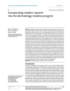
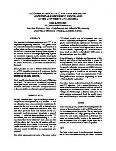
Eckel-Grossman risk task Before starting the experiment, students were given a PowerPoint

presentation with instructions on how the experiment would run. The presentation included both an introduction to a task that assessed their level of risk aversion and the auctions themselves. The risk aversion task was based on an instrument designed by Eckel and Grossman (2002). Figure 1 shows the task provided to participants at the University of Alberta, which was similar to the task provided to producers in the producer survey conducted in Miami, Manitoba. The task involved participants choosing between six gambles that are ranked from least to most “risky”. Each choice offered a simple gamble of a 50% chance of either a low payment or a high payment. As the size of the risk increases, the lower payment decreases and the higher payment increases. The expected return increased from gambles 1-5. The first gamble is a no risk gamble where there is a sure payoff of $2.80. The sixth gamble does not offer an increased expected return, only an increased risk above that of the fifth gamble choice. The most risky or gamble choice 6 offered a payment of either 20 cents or $7.00. Risk averse individuals are expected to choose gambles from 1-5, where the most risk averse individuals will choose gamble 1. Risk neutral bidders are expected to 23

choose either gamble 5 or 6 whereas risk seeking individuals would always choose gamble 6 (Dave et al. 2007). The risk task was different for the producers in the STC survey on two accounts. First, instead of completing the risk task on a computer like the participants in the experimental auctions, these were completed on paper. Secondly, the task was scaled up to a level that was expected to provide similar utility to the producers as the experimental levels would for students. The risk free gamble choice was a guaranteed payment of 14$ compared to the auction participants’ $2.80. The most risky gamble involved a payment of either 1 or 35$.

24

For this exercise you are asked to select from among six different gambles and choose the ONE gamble you would like to play. The six different gambles are listed below.  

You must select ONE AND ONLY ONE of these gambles. To select a gamble place an X in the appropriate box. Each gamble has two possible outcomes (Low Roll or High Roll) with the indicated probabilities of occurring. For example, if you select Gamble 4 and a High Roll occurs, you would be paid $26. If ROLL LOW occurs, you would paid $8. For every gamble, each ROLL has a 50% chance of occurring. To determine the payout, we would roll a ten-sided die to determine which event will occur. If a 1, 2, 3,4 or 5, is rolled, this will count as a Low Roll. Rolls of 6, 7, 8, 9 or 0, will count as High Rolls.

Roll Low High

Payoff $2.80 $2.80

Chances 50% 50%

Gamble 2

Low High

$2.40 $3.60

50% 50%

Gamble 3

Low High

$2.00 $4.40

50% 50%

Gamble 4

Low High

$1.60 $5.20

50% 50%

Gamble 5

Low High

$1.20 $6.00

50% 50%

Gamble 6

Low High

$0.20 $7.00

50% 50%

Gamble 1

Your Selection Mark only one gamble

Figure 1. Eckel-Grossman risk task for participants in the experimental conservation auctions conducted at the University of Alberta

25

3.2

Auction Methods

3.2.1

Experimental auctions Experimental economics are used to test the validity of economic theories

and better understand market mechanisms that are otherwise too expensive or impractical to research. In our case, experimental auctions were used to replace watershed level auctions. As a result, we were able to collect significantly more data and test a number of different treatments. Experimental auctions with students and University personnel may not directly provide evidence as to how producers would react during a “real” conservation auction. Previous experiments by Brookshire et al. (1987) and List and Shogren (1998) suggest that experimental auctions tend to be externally valid. 3.2.2

Auction Procedure Auctions were held at the University of Alberta in the Department of

Resource Economics and Environmental Sociology. Participants were undergraduate and graduate students and university employees. The auction experiments were completed using Z-Tree software (Fischbacher 2007). Auctions consisted of 12 participants and an auctioneer/buyer of conservation services. Experiments were scheduled to last an hour but usually lasted about 40 minutes. Participants were selected from an online database used in the Department of Resource Economics and Environmental Sociology using ORSEE software (Greiner 2004). Participants could only participate in the experiments considered in this thesis once to avoid any extra learning. However, students could have participated in previous auction experiments (e.g. Packman 2010; Boxall et al. 2013) Students have been used in other conservation auction research as well (Cason & Gangadharan 2004, 2005; Cason et al. 2003; Latacz-Lohmann & Schilizzi 2007 and Boxall et al. 2008) and are assumed to act similarly to a rational, profit maximizing firm/individual. Students and producers appear to perform in a similar manner in experimental conservation auctions (Boxall et al. 2008). 26

The auctions were framed as though students were representing farmers and were hoping to be paid for restoring wetlands. I was concerned about the possibility of environmental framing as an issue in the behaviour aspect of the auctions; however, Schilizzi et al. (2011) found that environmentally conscientious students do not tend to act significantly different from their less environmentally minded colleagues. With that in mind, the decision was made to frame the auction in such a manor so that students would have more of a reference point and it might make the experiments easier to understand. Packman’s thesis (2010) also framed experiments in a similar fashion. I felt consistency might prove to be valuable if comparisons were to be made between the two auction studies. A discriminatory payment mechanism was used; every period each successful participant was paid the amount that they bid. The alternative to discriminatory payments is uniform payments, which involves paying all successful bidders the same amount regardless of their bids. Usually, the amount paid is either the same as the highest accepted bid or the second highest. Despite the finding that uniform payment systems can outperform discriminatory payments in a budget based auction, discriminate pricing was chosen. I used discriminate pricing because in order to understand how changing costs affected behaviour and participation, I would need to provide payments where participants were directly affected by their decisions and the results of the realized costs. If participants were all paid the same amounts, they might not be affected as much by the actualized costs because they would be paid more than their bid and thus, much more than their expected costs. After the Eckel-Grossman risk task was completed, participants were given 5 practice periods in order to learn how the auction mechanism works, learn how the payments would translate into their cash payments and so experimenters could describe the auctions rules and functions. The actual experiment lasted for 18 periods in total. Each period of the auction lasted a maximum of 60 seconds; if 27

all participants submitted bids within the 60 second time limit the auction would clear and results would appear. Participants would experience rotating farms which meant that after 6 periods farm characteristics would change. Each set of 6 periods is called rounds in the discussion that follows. For 3 periods within each of those rounds the costs of restoration would not vary for each player, but could vary during the other 3 periods. This means that for 3 consecutive periods, the expected costs of implementation would not change after the auction cleared and successful bids were paid out. For the other 3 consecutive periods in that round, the realized costs after the auction cleared could be different from the expected costs given to the participants at the start of that period. 3.2.3

Experimental design The experiments used in this research constituted a 3 by 2 design. The

level of cost variation was one of the treatments and the other was the order in which participants were presented with potential cost variation rounds. Each session included rounds with some degree of potential cost variation. Sessions included rounds with 0% potential cost variation, and either 15% or 30% potential cost variation. In order to determine if the order in which cost variation was presented affected auction performance or bidder behaviour, half of the sessions had the potential cost variation in rounds first and the other half had the potential cost variation rounds presented second. Participants were provided with farm characteristics matching one of 12 chosen farms from the STC Watershed along with estimated costs of restoring all drained wetlands on these farms. The characteristics provided to participants included farm acreage, estimated total costs and unit (acre) costs. Participants were not given any parameters of the other farms nor information regarding the budget. The costs of restoration were scaled down to allow for an appropriate endowment to the participants at the University of Alberta. The actual costs were 28

divided by a factor of 800. Costs per acre of wetland restored ranged from $1.39 to $4.38. After completion of the first period, participants were given information regarding past performance. This information included whether or not they participated in the previous auction, their previous estimated costs, actualized costs, farm size, their previous offers, whether or not they won the auction, and their net income for previous auction periods. Participants received payment from three separate activities. First, each participant was paid an incentive of $5 for participating in the experiment. This payment was made regardless of their behaviour in completing the experiment. No participants ever chose to leave the experiment before completion. Secondly, students were paid for their “performance” in the auctions. Payments were not made every period, the software would randomly choose 3 periods, one from each of the three rounds. Participants were paid the sum of the three periods randomly chosen by the software. This allowed participants to get paid from each of the 3 farms they experienced during the session. This was important for fairness because some farms were more efficient than others and had a better chance of winning an auction than less efficient farms. Third; students received payments for their decision in the Eckel-Grossman risk task (EG). In order to encourage participants to behave realistically, they were offered payments based on auction results. The payment rule is shown below where I represent the random draw from each round:

[ ∑(

The screen presented to the participants would also indicate whether or not costs would vary in the following period. Furthermore, to reduce confusion, participants were informed verbally each time period if auctions switched from having no cost variation to having cost variation.

29

)]

Figure 2. Example of experimental auction participation choice and bid choice page in Z-Tree

Figure 3. Example of experimental auction result page in Z-Tree

30

Each experimental session had 18 periods, each period consisting of an auction. Each participant was given farm characteristics for 6 periods at a time. After 6 periods, farms would rotate and participants were given farms with new cost parameters. We designated each of these 6 period increments as rounds. Within each round, there would be 3 sequential periods of no cost variation and 3 periods of potential cost variation.

[

]

[

] [

]

[

] [

[

]

] [

]

Figure 4. Experimental design of changing farms

There were 12 subjects per session, each choosing whether or not to submit a bid every period. The potential analyses of these data consist of examining individual bidding behaviour across the 18 periods. In addition, one could treat the aggregate bidding behaviour of the 12 subjects in each period as an auction outcome. Thus, every auction period provided, for example, information about the efficiency of the auction that took place in that period.

[

]

[

]

[

]

Figure 5.Participant bids and auction outcomes for all 18 periods within a session

As mentioned above each auction also provided insight into the behaviour of individual participants. From the bids (or lack thereof) we can analyze how much participants were marking up their bids.

31

PMARKUP Auction outcomes based on aggregate bidder behaviour

Acre Cost PMOR Acres

Bidder behavioural outcomes

PMARKUP = ƒ(Risk Aversion, Potential Cost Variation,…)

Figure 6. Experimental auction level and individual level outcomes

There were two levels of potential cost variation that were tested along with the rounds with no potential cost variation. Each session had costs that varied using a discrete distribution that was almost normal. We were not able to use a randomized normal distribution in the experimental auctions because the experimental software did not have the capacity to include random inputs. There were 9 periods of either 15% or 30% potential cost variation in each experimental session and 9 periods without any potential cost variation, but an experimental session only used one of the cost variations to limit participant confusion. During periods of potential cost variation, costs could vary by zero, small, intermediate, or large amounts. For example; during the 15% potential cost variation periods, costs could vary by either 0%, 5%, 10%, or 15%; for the 30% level they could be 0%, 10%, 20%, or 30%. Costs could vary above or below the expected costs. The decision was made to have an almost normal discrete distribution of variances, the expectation was that most of the time producers would know their costs reasonably well; more often than not there would be little or no variation between expected and actual costs (see Figure 7). During potential cost variation periods: -

40% of participants would experience zero cost variation

-

33.4% of participants would experience a small level of cost variation. 32

-

16.6% of participants would experience an intermediate level of potential cost variation.

-

9.2% of participants would experience a large level of potential cost variation. 45 40 35

Percent of total

30 25 20 15 10 5 0 Large negative

Intermediate negative

Small negative

Zero

Small positive

Intermediate positive

Large positive

Level of cost variation Figure 7. Distribution of levels of potential cost variation for each session of experimental auctions at the University of Alberta

3.3

Survey Methods for Producers

3.3.1

Survey Design In order to establish actual producer risk aversion levels, the Eckel-

Grossman (2002) risk task was used which allowed us to compare their results with those from the experimental auction participants. We did choose to differentiate the University participant task from the producer task by increasing the payments for the producers proportionately as described above. We expected the vast majority of the University participants to be students, as was the case, and we expected producers to be well established, experienced farmers with higher 33

incomes, and thus, higher payoffs required to incent appropriate decisions. Other than the risk aversion task, a number of questions dealt with opinions of and experience with conservation auctions, BMP implementation, and environmental organizations and government departments. The rest of the survey solicited demographic information. The complete survey can found in Appendix 1. The target participants of the survey were producers farming in the WEBS STC watershed. Only 5 of those producers farming in the watershed were present at the meeting. The remaining 10 participants were residents of the area, but were not a part of the WEBS STC watershed. This was a contingency we considered when preparing for the survey. Researchers conducting the meeting where producers were gathered and surveyed expected upwards of 25 STC watershed producers and another 25 non-members. Participants were forthright about not being members of the STC, but were, however, all residents in the area. Most of the participant producers were Deerwood Soil and Management Association members. This group is relevant because as an organization they have dealt with and funded BMP implementation and have worked with the WEBs researchers. The producer survey was conducted in the town of Miami, Manitoba. Miami, is located near the outlet of the STC watershed, and is the closest town to the watershed. The survey was conducted over the course of one afternoon on January 10, 2013. The meeting was held at the Miami Community centre. Producers were gathered at the community centre because other WEBS modelling researchers from the University of Guelph were making a couple presentations. The first of which was made to producers interested in learning about BMP modelling with respect to their operations. The second presentation was for a wider audience of modellers, researchers, and government. 3.3.2

Survey Procedure Prior to attending the modelling presentations, producers in the STC

watershed were invited via letter to attend and participate in the survey. Producers 34

had already been invited to participate in the meeting, but a supplement letter was mailed out informing them about and inviting them to the survey portion. Only producers in the STC watershed WEBS project were sent the supplemental survey as that was the target group. After the modelling group form the University of Guelph completed their first meeting with producers, a brief presentation explaining conservation auctions was given to the producers and a request was made to participate in the survey. The survey was conducted in between the modelling presentations. Individuals choosing to participate in the auction came to the researchers and requested information and consent forms. They were given brief oral explanations of the information and consent forms and given time to read and complete them. Only after the consent forms were completed and returned to the researchers were the producers given the surveys. Producers completed the surveys on their own. Researchers were unable to monitor each participant directly, however, were available to answer questions as requested. There was some confusion with regards to the Eckel-Grossman risk task, but for the most part, producers had no trouble completing the surveys. Participants normally took about 5 minutes to read through and complete the information and consent forms. They spent approximately 30 minutes completing the survey. The data was collected and inputted into PSPP (Plaff & Darrington 2011). The analysis involved simple descriptive statistics and frequencies. The most important and relevant results from the producer survey were the results from the Eckel-Grossman risk task and information about how well producers knew or expected to know their costs. It is generally believed that knowledge of BMP costs at the producer level is producers have a very good understanding of their costs and that they wouldn’t perceive much uncertainty in BMP implementation.

35

Chapter 4. Results 4.1

Bidding Behaviour

4.1.1

Research Questions There is still limited research with regards to the effects of certain

treatments on conservation auctions, especially in the Canadian context. Bids in this study were selected based on the amount of wetland acreage restored, so coverage of some quantity measure. Submitted bids in each period were ordered by $ per acre from cheapest to most expensive. Since we worked with budget constrained auctions instead of target based auctions and used a discriminate payment rule, the cheapest bids ($/acre) were selected first up until the budget was exhausted. Thus, for this thesis the selection rule was based on wetland acreage restoration levels provided by individual farms. Bids submitted were based on a scenario where costs are derived from 100% of wetlands drained on each farm located in the STC study area. Obviously, 100% wetland restoration is unlikely in reality, however, with time and budget limitations, we decided to limit the number of treatments and increase the simplicity of the auctions to get the best understanding of the effects of risk aversion and potential cost variation on the auctions. This section will look at the statistical, graphical and econometric results of the experimental auctions conducted for this thesis. We will review the effects of risk aversion levels and levels of potential cost variation on bidding behaviour. For each of these variables, there is an associated hypothesis. 1. First, risk averse bidders are expected to bid closer to their costs, as suggested by the theory developed by Latacz-Lohmann and Van der Hamsvoort (1997). 2. Second, it is believed that bid levels will increase with increased levels of potential cost variation as bidders will fear losing money more than they hope to win the auction. 36

These two hypotheses appear to conflict with each other. One of the aspects of the research, increased risk aversion, is expected to reduce the size of bids. The risk involved here is that individuals are expected to be averse to not winning the auction. The other aspect, increased potential cost variation, is expected to increase the size of bids. The risk involved with the potential cost variation is the economic risk; there is the potential of losing money if the bid is lower than the realized cost. We analyze the effects of both risks during the econometric analysis of the experimental data where we can hold the effects constant. We generate a variable, percent markup (PMARKUP) to analyse the bidding behaviour of participants in the experimental auctions. PMARKUP, like markup in a commercial setting, describes the amount individuals add to their bid above the cost of implementing the restoration project in percentage terms. Below is the formula used to calculate PMARKUP: . 4.1.2

Summary Statistics We found that some students were bidding below their costs during the

experimental sessions. It is noteworthy that there were several cases where bids submitted were much lower than estimated costs. It is unclear why individuals would submit bids below their costs; however, our assumption is that participants were likely confused. It is possible that an individual might be bidding below their costs for any number of reasons. I attempted to alleviate this by observing participants during the auction sessions. When participants were consistently bidding below their estimated costs, the group would be reminded that in order to have a chance at making more than the base income, one would have to bid higher than estimated costs. For example, the experimenter would say “Just a reminder, in order to make more than your base salary, you will need to bid above your estimated costs”. Therefore, we would not state that participants should bid above their costs, only provide a reminder of how to earn a profit above the base income 37

in case of confusion with regards to the reverse auction mechanism. This usually eliminated the decision to bid below costs, suggesting that it was simply confusion with the mechanism. There were also some outlier bids on the positive side, a few individuals in some cases bid considerably higher than their estimated costs (e.g. 250%). These were likely “bogus” bids, where individuals were either confused by the auction, or they were aware they had no chance of winning the auction after a few attempts with the same farm characteristics. However, as mentioned in the experimental design, participants experienced new farms every six periods in an attempt to minimize this effect. 4.1.2.1

Eckel-Grossman and Potential Cost Variation Results As seen in Figure 8, levels of risk aversion for University of Alberta

participants are similar to those of producers in the STC watershed. The biggest differences appear at the lowest and highest levels of risk aversion. For the most “risk averse” group, there appears to be a higher percentage of producers than students and for the most “risk seeking” group, there is a higher percentage of students than producers.

38

30

University of Alberta Participants

Percentage of Participants

25

STC Survey Participants

20 15 10 5 0 1

2

3

4

5

6

Gamble Choice

Figure 8. Eckel-Grossman risk task gamble choice results of participants in percent of the experimental auctions at the University of Alberta and producers in the STC watershed, Manitoba

The results of the EG risk task might give us some insight as to how producers would react given certain conditions in a practical setting. It might be the case that the results of the experimental auctions could be similar to practical applications in the STC watershed. Obviously, as a few producers mentioned, the stakes involved in the risk task were not the same as they would be in a practical application. A conservation auction where farmers would be expected to change practices or their land has much greater implications than some “free money” from a researcher. However, more than 50% of producers still chose “risk averse” gambles and only one producer chose the “all or nothing” most risk seeking gamble. This could indicate that despite the reduced risk producers might have felt during the task, they would likely be more risk averse individuals overall. One of the hypotheses presented at the beginning of the thesis is that we expect more risk seeking individuals to seek more rent than their risk averse cohorts. Figure 9 demonstrates this relationship. 39

45 40 35 % Markup

30 25 20 15 10 5 0 1

2

3 4 Gamble Choice

5

6

Figure 9. Average percent markup sought across different levels of gamble choices on the Eckel-Grossman risk task

Figure 10 shows average bids per session for each of the 12 farms used in the experiments. The variation in the cost variation periods appears to be higher than that of the non-varied periods as more of the cost variation points lie above the 45 degree line in the graph, which depicts where costs would be equal to bids. Not only does there tend to be slightly more variation in the bids during cost variation rounds, but there tends to be more bids below costs. This could indicate some confusion with the auction, or an attempt to gamble that their costs will be lower than their expected costs, thus increasing their chances of winning more money in the auction.

40

80

70

60

Bids

50

40 No Cost Variation 30 Cost Variation 20

10

0 0

10

20

30 Cost

40

50

60

Figure 10. Average value of bids per session for cost varied and non-cost varied periods

Figure 9 and 10 show how markups appear to increase with higher levels of risk seeking behaviour, during rounds with potential cost variation. This is consistent with the theory proposed by Latacz-Lohmann and Van der Hamsvoort (1997). Both the hypotheses presented for bidding behaviour in this thesis are supported in Figure 10. Individuals choosing lower levels of the EG task tend to bid closer to their costs, whereas individuals who chose higher levels on the EG task seem to mark up their bids more substantially. Less obvious is the increase in 41

markups when there is potential cost variation is present. For the most part, markup increases for the no potential cost variation to the 15% level. However, it appears to remain flat or even decrease when the jump is made from the 15% level to the 30% level. Figure 11 addresses the question of the effect of potential cost variation on bids and the risk aversion variable on percent markup. It does this by combining the two variables. There are a number of observations to be made from this comparison. First is that the six gamble choices do not follow parallel paths. Risk seeking individuals appear to increase marking up their bids from when there is no cost variation the 15% potential cost variation. However, there seems to be a decrease in percent markup when the potential cost variation increased to 30%. This could indicate some confusion with the cost variation variable. Participants may not fully understand the risks involved in their bids, and are thus, more inclined to be “cautious” and bid closer to their costs. Second, most individuals choosing gambles 1-3 tend not to change their behaviour despite potential cost variation changes. Generally, these “risk averse” participants appear indifferent to potential cost variation, and choose to bid closer to their expected costs than their counterparts.

42

Gamble 1

Gamble 2

Gamble 3

Gamble 4

Gamble 5

Gamble 6

50 45 40

PMARKUP

35 30 25 20 15 10 5 0 0

15

30

Potential Cost Variation

Figure 11. Average PMARKUP during periods of 0, 15 or 30 percent potential cost variation sorted by gamble choices in the Eckel-Grossman risk task Zero Cost Variation

15% Potential Cost Variation

30% Potential Cost Variation

50 45 40 35 30 25 20 15 10 5 0 Gamble 1

Gamble 2

Gamble 3

Gamble 4

Gamble 5

Gamble 6

Figure 12. Average PMARKUP for various gamble choices in the Eckel-Grossman risk task across 0, 15 or 30 percent potential cost variation

43

4.1.2.2

Age and Gender The survey conducted at the end of the sessions allowed us to analyze

some of the demographic variables that might be affecting decision making during the auctions. We asked participants to provide their date of birth and gender. Age was considered as a potential factor in explaining behaviour. Sinha (1992) showed that individuals appear to become more risk averse as they age (Sinha 1992). We do see an overall decreasing trend in the gamble choice as participant age increases. Individuals aged 18-22 on average chose 4.0 and individuals aged 38-42 chose 3.0. Although there appears to be a decreasing trend in the gamble choices with age, approximately 88.5% of participants fell within the first three age groups of being between 18 and 32. We see the risk seeking attribute increase in the second group of participants aged 23-27 and then decrease again for participants aged 28-32. One individual fell in the age range of 53-57, and they chose the 6th gamble choice. A regression of risk aversion as a function of age shows that age is not a significant factor in the gamble choices for experimental auction participants. However, age was still included in the initial participation and bidding behaviour models to see if, despite their lack of significance on risk aversion, age might be another factor in bidding behaviour. A couple of things are noteworthy with regards to the gender demographic. First, the literature shows that males tend to be more risk seeking than females (Jianakoplos & Bernasek 1998; Sunden & Surette 1998). This appears to be supported in our research where we find that males more often chose the higher levels of the gamble choice in the Eckel-Grossman risk task. This finding, along with the evidence from the literature, provides justification for including gender as a variable in econometric models explaining bidding behaviour. However, the difference between male and female gamble choices was not statistically significant. Overall, the average gamble choice of participants was 3.91, which lies on the slightly more “risk seeking” side of the scale.

44

It is difficult to compare both the age and gender variables between the experimental auction group and the producer survey group. First, because University of Alberta participants included a large number of female participants (44.8%), but none of the producers in the STC survey were female. Secondly, the relative ages of the two groups was different, 25 percent of participants from the University exceeded the age of 30 and only two participants in the STC survey were less than 40 years of age. For a look at the results of the Eckel-Grossman risk task results for both groups grouped by age, see Appendix 3. 4.1.2.3

Learning Learning can also be an important factor in the conservation auctions

(Latacz-Lohmann & Schilizzi 2005; Hailu & Schilizzi 2005); particularly in experimental settings with repeated auctions. To capture the repeated nature of our experimental auctions we consider the sequence of periods within each round where the expected and or actual costs of adoption are held constant. Using this aspect of the design as an assessment of repeated auctions we find that PMARKUP decreases as the periods within a round elapse (Figure 12). This could indicate learning as periods progress. It appears as though participants learned to lower their bids in order to increase their chances of winning the auction as the session progressed. On average, PMARKUP appears to flatten out after the third period within a round; indicating participants finish learning about their position in the auctions by the third period.

45

40 35

PMARKUP

30 25 20 15 10 5 0 1

2 Period within a Round

3

Figure 13. Mean PMARKUP with 2 standard deviations above and below the mean as periods within rounds progress for the experimental auctions conducted at the University of Alberta.

We need to also consider the learning throughout the entire session of 18 periods. In Figure 13 we plot average PMARKUP for each of the three rounds, and find them to be lower in the 3rd round relative to the 1st round. This trend for both outcome variables is indicative of bidders decreasing their bids to be closer to their costs as the session progressed.

46

45 40

PMARKUP

35 30 25 20 15 10 5 0 1

2 Round

3

Figure 14. Mean PMARKUP with 2 standard deviations above and below the mean as rounds progress through sessions for the experimental auctions conducted at the University of Alberta.

Variables attempting to control for the repeated nature of the auctions within a session were also included in the regressions. Past experiments have shown that bidding behaviour changes over time as participants learn more about the auction and their costs (Hailu & Schilizzi 2005; Latacz-Lohmann & Schilizzi 2005; Reichelderfer & Boggess 1998). We found that PMARKUP tended to decrease as periods within rounds progressed (Figure 12) as well as rounds within the sessions (Figure 13). Thus, several variables were tested: periods within a session (18 periods), rounds within a session (3 rounds), and auction treatments within a round (2 treatments per round for 6 within a session). The periods within a round variable was used in the regressions below because learning appeared to occur within a round while expected or actual adoption costs were constant. All of these repeat measure variables were statistically significant in the regressions. The variables used to review the effects of learning and progression of auctions during a session were: the period within a round, lag of the cost 47

difference and lag of the adopted variables, and the interaction of the lagged PMARKUP with lag of adopted and the interaction of the lagged cost difference and lag adopted variables. The period within a round variable provides information on how behaviour might change from one period to the next. The lag of the cost difference is included to examine if changes in costs in the previous period have an effect on behaviour. 4.1.2.4

Econometric Analysis of Bids In order to help analyze the effect of several variables and variations of

those variables, I decided to display 3 models for PMARKUP. First, is a simple model that takes into account the research treatments, participant learning, and demographic variables collected during the experiment. The second model includes some lagged variables, and removes the demographic variables. Finally, a regression with the treatments, time – periods within rounds, the lagged variables and some lagged interaction variables are reported. For example, age and gender variables were included in the original regression, but were found to be insignificant and continued to be insignificant in subsequent regressions. Individual bids with greater than 250% markup were removed from the data set. These incidents could be chalked up to accidents or confusion when learning the auctions. The equation estimated is as follows with description of the variables in Table 1. Table 2 shows the results of 3 panel regressions of the PMARKUP variable using random effects error structure. Several regression models are shown to demonstrate the complex interactions between variables.

48

Table 1. Description of variables used in the empirical analysis of experimental conservation auctions Variable PMARKUP GAMBLE CHOICE

POTENTIAL COST VARIATION

AGE FEMALE TIME – PERIODS WITHIN ROUNDS LAG COST DIFFERENCE

LAG ADOPTED

LAG PMARKUP * LAG ADOPTED

LAG COST DIFFERENCE * LAG ADOPTED

VARIATIONFIRST

Definition Markup above costs in percentage terms Eckel-Grossman risk task gamble choice. Higher Gamble Choice indicates less risk aversion. Different levels of potential cost variation. Either no cost variation 0%, or potential variation – of up to either 15% or 30% for a given auction period. Age as provided by a brief questionnaire Gender dummy where Female=1 and Male=0 Periods within a round. 6 Periods per round. Used to determine if there is a learning effect. The difference in cost between the expected/estimated cost and the actualized cost in the previous period. Dummy variable for whether the participant’s bid was accepted in the previous period. 0=not accepted and 1=accepted Lagged interaction of the PMARKUP and Lag Adopted variables. A combination of the amount of markup of the individual and their winning of the auction. The coefficient is 0 for non-winners of the previous auction. Interaction of the Lagged Cost Difference and the Lagged Adopted variables. Combination of the cost difference between expected/estimated costs from the previous period and the winning of the auction. The value of this term is 0 for non-winners of the previous auction. Treatment for when potential cost variation periods occur before non-cost variation periods

49

The initial regression on PMARKUP included the GAMBLE CHOICE variable, the level of potential cost variation variable, the age and gender variables, and period within a round. On average, PMARKUP was about 20% as reported by the value of the constant in the model (Table 2). The level of potential cost variation and the demographic variables were not significant. The gamble choice variable was positive and significant at the 5% level. For each unit increase in the gamble choice on the Eckel-Grossman risk task, the percent markup increased by 1.2%. We did not include the treatment of which round had potential cost variation, either first or second (VARIATIONFIRST), because this variablenever was statistically significant in the regressions. Graphical analysis also showed that the round in which cost variation was included did not appear to have an effect on bidding behaviour. Table 2 Results of panel regressions, with random effects error structure, for PMARKUP

CONSTANT GAMBLE CHOICE POTENTIAL COST VARIATION AGE FEMALE TIME – PERIODS WITHIN ROUNDS LAG COST DIFFERENCE LAG ADOPTED LAG PMARKUP * LAG ADOPTED LAG COST DIFFERENCE * LAG ADOPTED Rho Overall R2

Coefficient (Std.Err) Intermediate Regression 19.221*** (2.895) 1.115* (0.660) 0.080* (0.044)

Initial Regression 20.094*** (8.697) 1.233** (0.678) 0.029 (0.040)

Final Regression 20.806*** (3.023) 1.319** (0.664) 0.091* (0.052)

0.040 (0.287) 0.034 (1.883) -1.839*** (0.333)

-

-

-

-

-1.957*** (0.394)

-2.330*** (0.457)

-

0.192 (0.128)

-0.092 (0.126)

-

5.231*** (0.822) -

-

-

-2.723 (1.922) 0.476*** (0.097) 1.184*** (0.339)

0.371 0.025

0.442 0.057

50

0.361 0.136

* Signifies statistically significant at 10% level, **Signifies statistically significant at 5% level, ***Signifies statistically significant at 1% level

The intermediate regression of PMARKUP left out the AGE and FEMALE variables for two reasons. First, neither demographics were significant in any form of the model. Second, neither of the demographics had an effect on the rest of the model’s results at any stage; they did not improve the fit or robustness of any regressions. The constant for PMARKUP is 19.2% and significant at the 1% level. Similarly to the initial regression, the gamble choice variable is both positive and significant at the 10% level. Individuals choosing higher gambles in the EG task tended to markup their bids more than their risk averse counterparts. More importantly, we now see a statistically significant effect of the potential cost variation in the rounds affecting bidding behaviour. The effect is small but significant at the 10% level. Participants mark-up their bids slightly more as the POTENTIAL COST VARIATION within a round increases. This could be an important finding. With the knowledge that potential cost varied in rounds had an effect on bidding behaviour, we can say that there may be an effect on producers’ risk perceptions in the way they form bids. If producers believe that there is little risk with respect to the cost of implementing the BMP or are very confident in knowing their costs, they will be less likely to markup their bids excessively. The assessment of the repeated nature of the experiments involved the periods within the rounds. As a reminder there were 6 periods in each round where the actual or expected costs of adoption were constant and there were 3 rounds. Therefore, the variable held integer values of 1 to 6. This period is negative and significant at the 1% level. PMARKUP decreases as each round progressed and is likely the result of early round excess rent seeking, which, would lead to a smaller likelihood of success in the auction. As a result, participants would begin to lower bids in order to increase their chances of winning the auction. 51

Since the goal was to understand the effects of bidding results and behaviour in previous experimental periods on current behaviour, the first lagged variable was the LAG COST DIFFERENCE which incorporated the difference in the expected or estimated cost and the actualized cost from the previous period. This variable is not statistically significant. However, the second lagged variable, the LAG ADOPTED is significant and positive. If the participant was successful in winning the previous period’s auction, they would mark-up their bids significantly in the current period. This makes sense intuitively; when they win an auction, they will choose to mark-up their bids slightly more the next round, testing the waters of the auction. The final regression included all of the variables of the intermediate regression and adds two additional lagged interaction variables. First, the constant is positive and significant suggesting that on average PMARKUP was 20.8%. Here, we find the GAMBLE CHOICE variable is positive and significant at the 5% level. The level of POTENTIAL COST VARIATION is also significant at the 10% level and positive. The TIME – PERIODS WITHIN A ROUND variable is negative and strongly significant at the 1% level. The LAG COST DIFFERENCE is not significant. This is a surprising finding; the cost differentials may not have been high enough to affect decision making behaviour. The biggest difference we see between the intermediate and final model is with the LAG ADOPTED variable. Previously, we saw that this variable was large, positive, and strongly significant. The lag adopted variable is negative in this case but not significant. However, this variable is interacted with two other lagged variables. One of these is the lag of the percent markup of the previous period. This interaction is both positive and strongly significant - the higher a participant’s markup from the previous period combined with winning the auction, the higher their markup would be in the current period. The LAG COST DIFFERENCE interacted with the LAG ADOPTED variable is both positive and significant at the 10% level. The higher the cost difference from the previous period combined with a participant winning the auction lead to higher markups in the current period. 52

Overall, winning in the previous auction period led to a lower PMARKUP in the current period. This is likely capturing the learning involved in the auctions where players get closer and closer to their final bid levels as the auctions progressed. 4.2

Auction Participation

4.2.1

Research Questions One of the major issues with conservation auctions is whether or not

administrating bodies will be able to attract enough participants to create competition to ensure expected efficiency gains from an auction. Prior experimental auction research did not allow for participants to make less money by participating, unless of course, participants bid below their costs. For this research, some participants did have the potential for lower net incomes as a result of participation. This could happen if bids were lower than actualized costs, yet still above estimated costs. There was, however, no possibility of losing money. Despite the possibility of making less than the base revenue in any given period, given the possibility of having total costs exceed total revenues, participants were given a financial incentive for participating in the auction and were able to make money for the risk aversion task at the beginning of the session (as well as the show-up fee). Thus, these experiments did not simulate an actual financial loss to students who performed poorly. The experiments did attempt to simulate what an actual producer’s decisions might look like when contemplating participating in a real conservation auction, however. The hypotheses presented for this section of the research are as follows: 1. Participants will choose to participate less during periods where their actualized costs could vary from estimated/expected costs. 2. Participants choosing the lower levels on the risk aversion task (risk averse) will be less likely to participate during the risk variable rounds than those choosing higher levels on the risk aversion task (risk seeking).

53

The first hypothesis is based on the expectation that for those periods where costs could vary, participants might see the potential cost variation as too risky to submit a bid. Although costs could decrease, and thus potentially increase overall revenues for the period, risk averse participants might be more conscientious of the potential cost increase rather than the decrease. Similarly, the second hypothesis expects that because the periods with potential cost variation might appear to be riskier, risk averse individuals could choose to avoid participation in the auction and simply settle for the base income provided each period. 4.2.1.1

Participation Results Participation rates were very high through all periods in the experimental

sessions – so high in fact that statistical comparisons of the potential cost variation and non-cost variation rounds did not seem useful. Throughout all eight sessions, bids were submitted 97.34% of the time. There were only 46 instances out of 1728 opportunities where bids were not submitted, which is only 2.66%. There was however, a slight decrease in participation as the sessions progressed. Female participants exhibited lower participation rates than male participants, which correlates well with two other results. First, male participants tended to have higher levels of the risk seeking attributes; and second it was found that participants with higher risk seeking attributes tended to participate more often than risk averse individuals. Both male and female participants decreased participation as the sessions progressed.

54

100 99

Participation %

98 97 Male

96

Female 95 94 93 1

2

3

Round

Figure 15. Participation rates (in terms of submitting a bid) between males and females from round to round during experimental auctions held at the University of Alberta

As mentioned above, participation rates were very high throughout the sessions. Despite the decreasing participation rates found in the experiments, participation remained higher than 95% for all periods except periods 11, 12, 15, 16, and 17. Averaged over the course of the sessions, the lowest level that participation ever fell to was 93.75%. Participation was 100% for 4 periods; 2, 3, 4 and 13. Participants tended to submit fewer bids when there is the risk of some cost variation. On average participation was 99.7%, 96.5% and 96.9% respectively for rounds 1, 2 and 3 where there was no potential for cost variation. Participation was, on average, 98.6%, 96.9% and 95.5% for rounds 1, 2 and 3 respectively during rounds where potential cost variation existed. The decreasing participation rates might indicate a degree of learning by participants, which could result from having lost out on revenue in previous periods. Participants may have also had trouble winning auctions in previous periods; which could lead to frustration and the decision to avoid participation altogether1. Using a chi-squared 1

Unfortunately, this was visible during one session. A researcher conducting the auctions noticed an individual who become frustrated with the results of the auctions.

55

test, the differences in participation rates between no potential cost variation and potential cost variation rounds are not statistically significant. The decreasing levels of participation from round to round are also not significant. 100 99

No cost variation

Participation %

98 97 96 95 94 93 1

2

3

Round

Figure 16. Percentage of participants submitting bids during rounds with no cost variation and rounds with cost variation

4.3

Auction Performance

4.3.1

Research Questions Not only are we interested in understanding how experimental bidders

behave under different treatments in an attempt to decipher how actual bidders behave; but we are also interested in understanding something about the overall effectiveness of the auction. This involves combining information from all of the bidders such that the economic efficiency and environmental effectiveness of the reverse auction can be assessed. Efficiency in the context of a conservation auction can be measured by a number of criteria. Some auctions aim for the maximum cost efficiency (cheapest cost per unit). Others simply aim to maximize the number of participants or contracts (e.g. Schilizzi & Latacz-Lohmann 2007). A number of limiting factors can affect the decision making factors when 56

selecting policies. This section of the thesis reviews some of the ways to assess the effectiveness of experimental conservation auctions by comparing auction level results among the different treatments of potential cost variation. 4.3.2

Auction evaluation measures One of the most important issues involved in the implementation of

auctions is the auctioneer’s scrutiny of bids in order to select the most cost efficient bids. There are several potential selection rules, such as maximizing some environmental output, maximizing some agronomic unit or, maximizing participation (Boxall et al. 2012). The analysis of the efficiency of the auctions in this thesis will primarily look at markup and unit cost of the auctions; however we will briefly touch upon other metrics such as the level of wetland restoration achieved. 4.3.3

Percent Markup (PMARKUP2) Information rent accumulated by producers during the auctions is an

important metric used to analyze the efficiencies of the auctions and compare the different treatments (Cason & Gangadharan 2004, 2005). Markup is defined as payments received by participants above what they would have been paid had they bid their costs. This allows policy analysts to review the auctions’ efficiency in their ability to achieve environmental benefits rather than provide producers with profit. In percentage terms it is calculated as:

∑

∑

[

∑

57

]

Table 3. Session level statistics for the experiments at the University of Alberta Session

1

Potential Cost Variation of Session (%) 0-15

2 3

PMARKUP2 Unit Cost (%) ($/Acre)

Average Gamble Choice

Number of Female Participants

Average age

15.6

2.0

4.417

3

27.4

0-15

19.3

2.0

4.250

5

26.6

0-30

13.3

1.9

4.167

8

25.6

4

0-30

15.6

2.0

3.500

7

24.4

5

0-15

21.7

2.1

4.083

6

26.2

6

0-15

21.3

2.1

3.833

7

24.1

7

0-30

22.6

2.1

3.500

6

25.3

8

0-30

19.8

2.1

3.583

2

25.8

Average

NA

18.7

2.0

3.917

5.5

25.7

One of the variables involved in determining the effectiveness of the auctions is the average risk aversion level established from the gamble choice variable of a particular session. Figure 16 shows the results of the sessions with respect to average gamble choice. There is a decreasing trend with respect to PMARKUP2 as the average gamble choice of a session increases. This indicates that, as a group, the less risk averse they were, the higher the bids they submitted were higher than their costs.

58

25

PMARKUP2

20 15 10 5 0 3.50

3.50

3.58 3.83 4.08 4.17 AVERAGE GAMBLE CHOICE

4.25

4.42

Figure 17. Average group level PMARKUP2 at the auction level relative to the average gamble choices of participants for each session.

Another important variable to review with respect to PMARKUP2 is the effect of the treatment of potential cost variation. Overall, it appears as though PMARKUP2 is higher during periods with potential cost variation. It is unclear why PMARKUP2 is lower for the periods with the high potential cost variation than they are during the periods with the low potential cost variation. The Period variable is also important in the analysis of the auctions. From a policy perspective, it could be important to understand how auctions perform as they are repeated. Similarly to actual producers, participants in the experimental auctions might learn about other participants’ costs, learn about where they stand with respect to their own costs and farm performance among bidders in the pool. A number of papers review repeated auctions and the consensus seems to be that auction performance erodes as time passes (Cason & Gangadharan 2004, 2005; Cummings et al. 2004; Hailu & Schilizzi 2005; Latacz-Lohmann & Schilizzi 2007). As a result of these findings, the hypothesis is that learning will occur with repeated auctions resulting in higher markups. Figure 17 shows this deterioration – PMARKUP2 increased as the periods progressed through the rounds.

59

AVERAGE PMARKUP2

25 20 15

No Potential Cost Variation

10

Small Potential Cost Variation

5

Large Potential Cost Variation

0 1

2

3

PERIOD WITHIN A ROUND

Figure 18. Average group level PMARKUP2 for different levels of potential cost variation through periods within rounds where potential cost variation periods occur first. 30

AVERAGE PMARKUP2

25 20

No Potential Cost Variation

15 10

Small Potential Cost Variation

5

Large Potential Cost Variation

0 1

2

3

PERIOD WITHIN A ROUND

Figure 19. Average group level PMARKUP2 for different levels of potential cost variation through periods within rounds where potential cost variation periods occur second.

60

4.3.4

Unit Cost We can further estimate the efficiency of the auction by looking at the per

unit cost, or cost per wetland acre restored. This was assessed using the following relation: ∑ ∑ This research will evaluate the acres achieved per dollar spent in the auctions. Recall that the selection criterion was the cheapest per unit cost. Bids were accepted until the budget was exhausted. Like PMARKUP2, we can look at the unit cost of the auctions with respect to the average gamble choice, the periods within the rounds and the potential cost variation variables. Figure 19 and 20 below show the amount in dollars spent per acre achieved in a particular auction. The amount that each acre achieved appears to decrease the more risk seeking a group is for a given auction. The change in the unit cost of an acre achieved is much more visible when we analyze the time variable. As the period within a round progressed, the unit cost of an acre restored appears to increase.

61

Average UNIT COST ($/Acre Restored)

2.15 2.1 2.05 No Potential Cost Variation

2 1.95

Small Potential Cost Variation

1.9

Large Potential Cost Variation

1.85 1.8 1

2

3

Period within a Round

Average Unit Cost ($/Acre Restored)

Figure 20.Average UNIT COST at the auction level for periods within rounds where potential cost variation periods occurred first. 2.12 2.1 2.08 2.06

No Potential Cost Variation

2.04 Small Potential Cost Variation

2.02 2

Large Potential Cost Variation

1.98 1.96 1

2

3

Period within a Round

Figure 21. Average Unit Cost at the auction level for periods within rounds where potential cost variation periods occurred second.

4.3.5

Econometric Analysis In their paper reviewing the economic efficiency of auctions, Cason &

Gangadharan (2005) used a panel regression model with a random effects error structure for the experimental session. The random effects structure was used to 62

take into account potential correlation within a particular group of experimental participants (Cason & Gangadharan 2005). In order to account for the potential different levels of clustering, we included SESSION (8 Sessions) and NROUND (sets of 6 auction periods) in a three-level mixed regression. The model has two random-effects, one nested in the other. The first is the SESSION (level three) and the second is NROUND (Level two) and is nested within SESSION. The remaining level contained the fixed effects which are the other right hand side variables that varied among the periods. It is assumed that the results of the auction were a function of the potential cost variation treatment, the period within a round during a session and the average risk aversion levels of participants within a session. For the auction level regressions, we will also look at the effect of the interaction of the potential cost variation of a given period and the average risk aversion level of participants in a session. Below in Table 4 is a description of the variables used in the analysis of the auction level results. We also test the random effects of several parameters. First we include a SESSION effect which accounts for each of the 8 experimental sessions that we ran. Second, nested in the sessions is NROUND, which is a variable for each set of 6 experimental auctions when farm parameters remained the same. There are a total of 24 sets of NROUND. For example, for the first session, there will be 3 sets of NROUND of 1,1,1,1,1,1 then 2,2,2,2,2,2 then 3,3,3,3,3,3 for a total of 18 periods.

63

Table 4. Description of variables used in the empirical analysis of experimental auctions conducted at the University of Alberta Variable

Description

PMARKUP2

Percent markup of Payments made above actual costs in percentage terms Dollars spent per acre of wetland restored Different levels of potential cost variation. Either no cost variation 0%, or up to 15% or up to 30% for a given auction period. Eckel-Grossman risk task gamble choice. Higher Gamble Choice indicates less risk aversion among the sample of subjects. Interaction of the potential cost variation and the average gamble choice variable Sets of 3 consecutive experimental auction periods. Used to determine if there is a learning effect.

UNITCOST POTENTIAL COST VARIATION

AVERAGE GAMBLE CHOICE

POTENTIAL COST VARIATION * AVERAGE GAMBLE CHOICE AUCTION

Individual demographic variables like gender (count of females in a session) and average age were collected but not used in the analysis because they can tend to be difficult to index to the aggregated session level and we found those variables to be insignificant in explaining individual bidding behaviour. Regression parameters were estimated using Stata 11.0.

64

Table 5. Results of panel regressions, with multi-level random effects error structure for PMARKUP2 and Unit Cost

Coefficient (Std.Err)

Variable

PMARKUP2 44.778* (16.331) -6.789 GAMBLE CHOICE (4.140) -1.258* POTENTIAL COST VARIATION (0.502) 0.345* GAMBLE CHOICE*POTENTIAL (0.132) COST VARIATION -0.139 AUCTION (0.626) Estimate Random-Effects Parameters (Std. Err.) 3.217* SESSION (0.129) 1.998* NROUND (0.931) 6.132* Residual (0.401) * Signifies statistical significance at the 5% level or beyond CONSTANT

Unit Cost 1.448* (0.163) -0.068 (0.041) -0.013* (0.005) 0.003* (0.001) -0.001 (0.006) Estimate (Std. Err.) 0.032* (0.013) 0.020* (0.009) 0.061* (0.004)

The constant for PMARKUP2 was about 45%, and was significant at the 1% level. This indicates that a significant amount of markup was being sought by the bidders during the sessions. As can be seen in Table 5 the average GAMBLE CHOICE was not statistically significant for PMARKUP2 at the auction level. POTENTIAL COST VARIATION was negative and significant. For each percent increase in potential for cost variation, PMARKUP2 decreased by about 1.3%. The GAMBLE CHOICE*POTENTIAL COST VARIATION variable was significant and worked in the opposite direction as the POTENTIAL COST VARIATION on its own. PMARKUP2 is higher on average when GAMBLE CHOICE and POTENTIAL COST VARIATION are combined and increasing. PMARKUP2 decreases as auctions progress within a round.

65

The average UNIT COST for an acre of wetland restored in the experiments was about 1.45$/acre in experimental dollars. Similar to PMARKUP2, the risk aversion variable was not significant for unit cost. Also similar to PMARKUP2, the potential for cost variation had a negative effect on unit cost. An increase of POTENTIAL COST VARIATION by 1% decreased the unit cost of the auction by about 13 cents/acre. The interaction of the risk variables was also significant and positive with respect to UNIT COST. Lastly, the AUCTION variable was not statistically significant. 4.3.6

Auction Acreage Achieved Maximizing the level of environmental improvement for the budget spent,

or in this case the number of wetland acres restored, is another potential goal for policy makers. In our case, we do know the wetland acreage that could be restored associated with each bidder. However, without this knowledge, policy makers can still easily access how many acres of wetlands were restored. This is an easily reported statistics and is quite accessible information for the public. The acres achieved variable is the amount of participants that won the auction multiplied by the amount of acres assigned to the farms of those participants that won the auction. Figure 21 shows restoration acreage achieved during rounds with different levels of potential cost variation. The amount of acres restored during rounds with no potential cost variation is higher than those rounds where costs could vary. The average acreage restored during non-risk rounds was 39.9 acres. The average amount of acres restored during rounds with potential cost variation is lower than the non-cost variation rounds. For the low level of potential cost variation, we see an average of 38.1 acres; for the high level we see 38.8 acres restored. However, there is no statistically significant difference between the number of acres restored during no cost variation and potential cost variation periods. Overall, the average acreage achieved was 39.16 acres.

66

45 40

Acres Achieved

35 30

No Potential Cost Variation

25 20

Small Potential Cost Variation

15

Large Potential Cost Variation

10 5 0 1

2

3

Period within a Round

Figure 22. Auction level average number of acres restored (an assessment of environmental objectives achieved) for different levels of potential cost variation for the experimental auctions where potential cost variation periods occurred first. 45 40

Acres Achieved

35 30

No Potential Cost Variation

25 20

Small Potential Cost Variation

15

Large Potential Cost Variation

10 5 0 1

2

3

Period within a Round

Figure 23. Auction level average number of acres restored (an assessment of environmental objectives achieved) for different levels of potential cost variation for the experimental auctions where potential cost variation periods occurred second.

4.3.6.1

PMOR Acres We also examine a statistic used by Cason and Gadharan (2005) to

analyze auction treatments called the proportion of the maximum objective 67

realized (PMOR). The maximum objective used in the calculation of PMOR is the maximum acreage restored given the budget of the auction, assuming participants bid their costs. As a result it tells policy makers how efficient the auctions are at achieving environmental outcomes. PMOR is defined as:

where i is the period. Given the budget constraint, and farm costs, we can calculate the maximum achievable if participants were to bid their costs. Given a budget of $100 and assuming each participant submitted bids equal to their costs, the amount of acreage achieved would be 52.82 acres, the budget spent would be $91.03 in experimental dollars, and there would be eight adopting participants. On average the proportion of the maximum possible acres across all sessions was 74.14%. The proportion of acres achieved was higher for rounds with zero potential cost variation at 75.5%. It was 72.1% and 73.5% for the low and high potential cost variation rounds respectively. 90 80 70 60

No Potential Cost Variation

50 Small Potential Cost Variation

40 30

Large Potential Cost Variation

20 10 0 1

2

3

Figure 24. Auction level average PMOR of acres restored where potential cost variation periods occurred first.

68

90

PMOR Acres Achieved

80 70 60

No Potential Cost Variation

50

Small Potential Cost Variation

40 30

Large Potential Cost Variation

20 10 0 1

2

3

Figure 25. Auction level average PMOR for acres restored where potential cost variation periods occurred second.

4.4

Producer Survey

4.4.1

Survey Design The producer survey had two major components. The first component

involved was eliciting risk aversion levels of producers in the South Tobacco Creek watershed. This was accomplished using the same Eckel-Grossman tool as used on participants in the experimental auctions at the University of Alberta. The Eckel-Grossman risk task was scaled up from what participants at the University were offered. Most participants in the auctions were students, whereas participants in the survey were farm operators in the area surrounding Miami, Manitoba. After completing the risk task there were a number of questions regarding conservation auctions, BMPs, farm characteristics and demographics. 4.4.2

Survey Results The first part of the survey was the Eckel-Grossman risk task. Second, the

next six questions had to do with experience and opinions of conservation 69

auctions and BMPs. Following that, the rest of the survey, questions seven through seventeen are producer demographic and farm demographic questions as well as a few opinion questions with regards to potential organizations to deliver agri-environmental programs. To review the complete producer survey results, see Appendix 2. The most important aspect of the survey was to establish risk aversion levels of producers to allow us ground truth the results from the experimental auctions. Unfortunately, only one third of the survey participants were producers represented in the data used in the experimental auctions. However, of the producers that completed the survey, all were from the area surrounding the STC watershed, near Miami and Morden, Manitoba. Results of the producer survey Eckel-Grossman risk task are shown and compared to the University participant results in Figure 8. Question 1) BMP and Auction participation table After completing the risk aversion task, producers were asked to fill out a brief table which outlined seven BMPs and asked 3 questions about each one. The seven BMPs included six of the BMPs tested on the STC watershed plus the wetland restoration BMP. A brief description of each of the BMPs was included on the back page of the survey in Appendix 1. Table 6 lists the BMPs included in the survey. Table 6. BMPs included in the producer survey BMP Category Riparian Vegetation Management Improved Cropping Systems Perennial Cover / Cover Crops Winter Bale Grazing Runoff Retention Pond Small Reservoirs Wetland Restoration - Farmyard Runoff Control

70

The three questions asked about the BMPs listed above are below: -

Have you participated in an auction related to this BMP? (Y/N)

-

Would you participate if an auction was offered for this BMP? (Y/N)

-

Do you know what your costs would be if you adopted this BMP? (Y/N)

Part of the reason of conducting the survey was to establish an introductory understanding of producers’ experience with and understanding of conservation auctions. Few participants in the watershed indicate having any experience with practical auctions for BMPs. Zero participants indicated having participated in an auction for riparian vegetation management, perennial cover/cover crops, winter bale grazing, holding ponds, small reservoirs or wetland restoration. The only practice with any indication of having participated in an auction was the improved cropping systems auction. Two of the fifteen producers indicated having completed an auction for improved cropping systems. The second statement with respect to the BMPs asks about producers’ willingness to participate in an auction if one were offered. This question might not be an accurate portrayal of how producers would react in a practical setting, but it gives an impression of their willingness to participate. More participants said they would than would not participate in auctions for the following BMPs were they offered: -

Improved Cropping Systems Perennial Cover / Cover Crops Runoff Retention Pond Small Reservoirs

More producers were unwilling to participate in auctions for the following BMPs were they offered: -

Riparian Vegetation Management Winter Bale Grazing

Seven producers indicated they would participate and seven said they would not participate in an auction for wetland restoration. 71

Table 7. Producer stated willingness to participate in an auction for different BMPs BMP Category Description

Would you participate in an auction if it were offered?

Riparian Vegetation Management Improved Cropping Systems Perennial Cover / Cover Crops Winter Bale Grazing Runoff Retention Pond Small Reservoirs Wetland Restoration Farmyard Runoff Control

Yes 5

No 7

Missing 3

11

2

2

10

3

2

4 7 10 7

9 5 3 7

2 3 2 1

The final part of this question asked whether or not participants would know their costs of implementing the set of BMPs. Producers indicated they might not know their adoption costs with respect to all the BMPs listed. Most producers indicated not knowing their costs for all the BMPs except the improved cropping systems BMP, where more producers indicated knowing their costs. Table 8. Producer stated knowledge of costs of BMP implementation BMP Category Description

Do you know what your costs would be if you adopted this BMP? Yes No Missing

Riparian Vegetation Management Improved Cropping Systems

5

6

4

6

5

4

Perennial Cover / Cover Crops

5

6

4

Winter Bale Grazing

2

6

7

Runoff Retention Pond

3

8

4

Small Reservoirs

3

9

3

Wetland Restoration Farmyard Runoff Control

3

8

4

Question 2) What range of cost uncertainty in percent would you be willing to accept for you to participate in an auction [ex: 10% above or below what you expect your costs to be]?

72

It would have been preferential to complete this (as well as the rest of the survey) prior to conducting the experimental auctions at the University of Alberta because then we could have used the information from the survey to help with the auction design. However, we can still compare the producers’ responses to the variations used during the experimental auctions. On average, producers indicated that the acceptable level of potential cost variation they would accept in participating in a conservation was 12.25%. The minimum stated level was 5% and the maximum was 20%2. Chapter 5. Discussion and Conclusions 5.1

Summary and Implications In an attempt to understand the effects of risk aversion and potential cost

variation in conservation auctions, I adapted experiments conducted by other students in the department of Resource Economics and Environmental Sociology. Using an adapted Eckel-Grossman (2002) risk task, I developed estimates of risk aversion levels for participants prior to completing the auctions. Below is a brief discussion of the results and their implications. 5.1.1

Cost Variation One of our main objectives was to understand how participants would

react to different potential cost variation scenarios. As discussed earlier in the Introduction, the purpose of introducing potential cost variation into the auctions is because adoption costs are likely to be uncertain to both producers and auctioneers. The expectation that auctions will be efficient is based the fact that costs are known to the producers. Therefore, it is important to understand how the potential for lack of knowledge of both present and future costs, could affect the performance of conservation auctions. Other research is being conducted on the 2

One producer indicated that they would be willing to participate in an auction with potential cost variation of anywhere from 10% to 80%, these values were not included in the average percent nor the maximum because of its extreme range.

73

costs of implementing BMPs and to better understand their economic and environmental benefits and costs. However, it may be helpful for policy makers and producers to understand how much their adoption costs could vary. This would help policy makers design auctions for BMP procurement. I found that potential cost variation affected individual bidding behaviour as well as the overall performance of auctions. Regression analysis showed that participants’ percent markup increased positively with potential cost variation. However, I found that the increase in markup did not continue at higher levels of potential cost variation. It does appear that the higher the potential costs of variation (lack of knowledge of costs), the more participants bid above their costs. At the auction level, the percent markup of payments to participants decreased with potential cost variation. The implication of this is that “riskier” auctions will result in lower overall percent markup in terms of those who got paid. In other words, when the potential cost variation increases, actual payments to participants decreased. This is likely due to higher individual percent markup which lowers the number of bids acceptable to the auctioneer and only offers payments to those with very low percent markup. It may be the case that some BMPs have little or no potential cost variation and others may have large cost variations. Understanding which BMPs exhibit this characteristic would be an important result for widespread use of conservation auctions in incenting BMP adoption. Results from the survey indicate that producers appear to be willing to accept a degree of potential cost variation; on average the level of cost variation that was stated to be acceptable to producers was about 12%. It is likely that if producers were aware that the costs of a particular BMP could vary by as much as 30% (as was presented in some of the experiments) it is unlikely there would be high levels of bidder participation in the auction, or this variation could affect the effectiveness of bidding behaviour and the effectiveness of the auction. Potential cost variation also negatively affected the unit cost of the environmental improvement in the auction.

74

5.1.2

Risk Aversion Risk aversion was established for both participants in the conservation

auction experiments and for a sample of producers in the South Tobacco Creek watershed. Understanding how risk aversion would affect the behaviour of participants in the experimental auctions could be important in understanding how producers would react to more “risky” conservation auctions. If producers do not have a good appreciation of their potential implementation costs or accept that their costs could vary after signing a contract, they may react differently depending on risk aversion. Generally speaking, we found that risk averse bidders submitted bids closer to their costs and that more risk seeking individuals were marking up their bids. For each increase in the gamble choice (increase in risk seeking tendencies), participants on average, marked up their bids by 1.3%. Risk aversion did not appear to have an effect on the overall effectiveness of the auction. A brief survey of some of the producers in the South Tobacco Creek Watershed found that producers and student participants exhibited similar distributions for the Eckel-Grossman risk task. Furthermore, in previous experiments, it was discovered that student participants began to behave like farmers after 2-3 periods (Boxall et al. 2008). Hopefully, this means that the experimental results will translate reasonably well into practical applications of conservation auctions. This could help policy makers better appreciate conservation auctions capacity as price discovery of EG&S and their efficiency in procurement of those benefits. 5.2

Limitations and Further Research The main limitations of this research are the limited capacity for further

data collection. First, it would have been valuable to complete more experiments and test the effects of the different treatments more thoroughly. Second, we were not able to collect enough data from producers in the watershed. The main goal of

75

the survey was to establish risk aversion levels of producers in the South Tobacco Creek Watershed, and we were only able to survey 15 producers. The experimental design employed appeared to be effective. The main concern with the experimental component of the overall study was the limited effect of the larger potential cost variation of 30%. We also think that information is needed on the distribution of costs for goods and services to be used in auctions. We used a normal distribution, but there is no information on whether this distribution is similar to actual distributions of adoption costs or cost errors in the real world. Producers indicated that they would be willing to accept up to about 12% cost variation. Participants were marking up their bids more with the 15% and 30% cost variation treatments; however, markup was not significantly higher for the 30% periods. We also expected to see participation rates drop as potential cost variation was introduced, but this was not the case. Although we found slight decreased levels of participation, it was not significantly different than when potential cost variation was present, and remained very high, above 95% participation. This could be one of the drawbacks of experimental settings where “losing” may be deemed more serious than “winning”, hence high levels of participation would be observed. The participants in the experimental auctions were “playing” with relatively small dollar amounts. Although we attempted to increase the realistic nature and induce “risky’ decisions, this might not have been the case because the dollar amounts were so small. As a result, students may not have been performing realistically and reacting to the risk appropriately. Furthermore, there were no significant penalties for performing poorly in the auctions (bidding below costs). This was a result of the ethical implications of taking away money from participants, but also the randomized nature of the draws for payments from only 3 periods. The show up incentive and the EckelGrossman task payment insured that no participants left without some cash in their pockets. Normally, producers would not only have to decide to participate in an auction, but may also have to decide whether to participate in session describing the auction and what it entails. Our auction design essentially forces 76

participants to show up every period, and then offers a decision of whether or not to participate. Further experiments using “more risky” attributes or practical applications of conservation auctions could provide more valuable information as to how potential cost variation could affect behaviour and auction efficiency.

77

Literature Cited Antle, J. M. 1987. Econometric estimation of producers' risk attitudes. American Journal of Agricultural Economics, 69: 509-522. Arrow, K. J. 1971. Essays in the Theory of Risk-bearing (Vol. 1). Chicago: Markham Publishing Company. Ausubel, L.M. & P. Cramton. 2002 “Demand reduction and inefficiency in multiunit auctions”. Mimeo, University of Maryland. Bard, S. K., & P.J. Barry. 2001. Assessing farmers' attitudes toward risk using the" closing-in" method. Journal of Agricultural and Resource Economics, 26: 248-260. Bardsley, P. and M. Harris. 1987. An approach to the econometric estimation of attitudes to risk in agriculture. Australian Journal of Agricultural and Resource Economics, 31: 112–126 Binmore, K. & J. Swierzbinski. 2000. Treasure auctions: Uniform or discriminatory? Review of Economic Design, 5: 387-410. Binswanger, H. P. 1980. Attitudes toward risk: Experimental measurement in rural India. American Journal of Agricultural Economics, 62: 395-407. Binswanger, H. P., & D.A. Sillers. 1983. Risk aversion and credit constraints in farmers' decision‐making: A reinterpretation. Journal of Development Studies, 20: 5-21. Bond, G. E., & B. Wonder. 1980. Risk attitudes amongst Australian farmers. Australian Journal of Agricultural and Resource Economics, 24: 16-34. Boxall, P. O. Perger, M. Weber. 2012. An experimental examination of target based conservation auctions. Department of Resource Economics and Environmental Sociology, University of Alberta, Edmonton. Retrieved from http://www.rees.ualberta.ca/Research/~/media/rees/Research/Documents/Staff%2 0Papers/SP-12-01.pdf Boxall, P., O. Perger, & M. Weber. 2013. Reverse auctions for agri-environmental improvements: selection rules and pricing for beneficial management practice adoption. Canadian Public Policy. In Press. Boxall, P., M. Weber, O. Perger, M. Cutlac, & A. Samarawickrema. 2008. Results from the farm behaviour component of the integrated economic hydrologic model for the watershed evaluation of beneficial management practices program: summary of phase 1 progress. Department of Rural Economy, University of 78

Alberta. Retrieved from http://www.rees.ualberta.ca/en/Research/~/media/rees/Research/Documents/Proje ct%20Reports/PR-08-01.pdf Brookshire, D.S., D.L. Coursey, & W.D. Schulze. 1987. The external validity of experimental economic techniques: analysis of demand behaviour, Economic Inquiry 25: 239–250. Brown, L.K. R. Troutt, C. Edwards, B. Gray & W. Hu. 2011. A uniform price auction for conservation easements in the Canadian Prairies. Environmental and Resource Economics 50: 49-60. Bulow, J.L. & D.J. Roberts. 1989. The simple economics of optimal auctions. Journal of Political Economy, 97: 1060-90. Cason, T.N. & L. Gangadharan. 2004. Auction design for voluntary conservation programs. American Journal of Agricultural Economics, 86: 1217-1222. Cason, T.N. & L. Gangadharan. 2005. A laboratory comparison of uniform and discriminative price auctions for reducing non-point source pollution. Land Economics, 81: 51-70. Cason, T.N., L. Gangadharan, & C. Duke. 2003. A laboratory study of auctions for reducing non-point source pollution. Journal of Environmental Economics and Management, 46: 446-471. Cornerford, E. 2013. The impact of permanent protection on cost and participation in a conservation programme: A case study from Queensland. Land Use Policy, 34: 176-182. Cummings, R.G., C.A. Holt, & S.K. Laury. 2004. Using laboratory experiments for policy making: An example from the Georgia irrigation reduction auction. Journal of Policy Analysis and Management, 23: 341-363. Dave, C., Eckel, C., Johnson, C., & Rojas, C. 2007. On the heterogeneity, stability, and validity of risk preference measures. Unpublished manuscript. Department of Economics, University of Texas at Dallas. David, E., & Sarne, D. 2010. The choice of eliminating the uncertainty cloud in auctions. In Agent-Mediated Electronic Commerce. Designing Trading Strategies and Mechanisms for Electronic Markets (pp. 15-28). Springer Berlin Heidelberg. Chetan, D., C. C. Eckel, C.A. Johnson, & C. Rojas. 2010. Eliciting risk preferences: When is simple better? Journal of Risk and Uncertainty, 41: 219-243

79

Eckel, C. C., & P.J. Grossman. 2002. Sex differences and statistical stereotyping in attitudes toward financial risk. Evolution and Human Behavior, 23: 281-295. Environomics Research Group Limited (Environomics). 2006. National survey of farmers and ranchers: Ecological goods and services. Report Number pn5742. Prepared for Wildlife Habitat Canada May 2006. Esö, P., & L. White. 2004. Precautionary bidding in auctions. Econometrica, 72: 77-92. Fischbacher, U. 2007. z-Tree: Zurich toolbox for ready-made economic experiments. Experimental Economics, 10: 171-178. Farm Service Agency (FSA). 2013. Monthly Summary – April 2013 of Conservation Reserve Program. Accessed at: http://www.fsa.usda.gov/Internet/FSA_File/apr2013crpstat.pdf. Greiner, Ben, 2004. "An Online Recruitment System for Economic Experiments," MPRA Paper 13513, University Library of Munich, Germany. Groth, M. 2005. Auctions in an outcome based payment scheme to reward ecological services in agriculture: Conception, implementation, and results. 45th Congress of the Regional Science Association, Amsterdam, 23-27 Aug. 2005. Hartwell, R. & B. Aylward. 2007. Auctions and the reallocation of water rights in central Oregon. Deschutes River Conservancy, River Paper Series No.1. Hailu, A. & S. Schilizzi. 2005. Learning in a “Basket of Crabs”: An agent-based computational model of repeated conservation auctions. In Lux,T., E.Samanidou, S. Reitz. Series: Lecture notes in economics and mathematical systems: Nonlinear dynamics and heterogeneous interacting agents (27-39). Berlin, Heidelberg: Springer. Hill, M.R. J., D. G. McMaster, T. Harrison, A. Hershmiller & T. Plews. 2009. A reverse auction for wetland restoration in the Assiniboine River Watershed, Saskatchewan. Canadian Journal of Agricultural Economics 59: 245-258. Jianakoplos, N. A., & A. Jerrnasek. 1998. Are women more risk averse? Economic Inquiry, 36: 620-630. Kim, J., & Y.K. Che. 2004. Asymmetric information about rivals' types in standard auctions. Games and Economic Behavior, 46: 383-397. Klemperer, P. 1999. Auction theory: A guide to the literature. Journal of Economic Surveys, 13: 227-286. 80

Kocher, M. G., Pahlke, J., & S.T. Trautmann. 2010. An experimental test of precautionary bidding. Accessed from http://hdl.handle.net/10419/37164. Latacz-Lohmann, U. & C. Van der Hamsvoort. 1997. Auctioning conservation contracts: A theoretical analysis and an application. American Journal of Agricultural Economics, 79: 407-418. Latacz‐Lohmann, U., & C. Van der Hamsvoort. 1998. Auctions as a means of creating a market for public goods from agriculture. Journal of Agricultural Economics, 49: 334-345. Latacz-Lohmann, U. & S. Schilizzi. 2005. Auctions for conservation contracts: A review of the theoretical and empirical literature. Report for the Scottish Executive Environment and Rural Affairs Department, Project No.: UKL/001/05. 150. Accessed at http://www.scotland.gov.uk/Publications/2006/02/21152441/0 Latacz‐Lohmann, U., & S. Schilizzi. 2007. Quantifying the Benefits of Conservation Auctions EuroChoices, 6: 32-39. Levin, D & J.L.Smith. 1994. Equilibrium in auctions with entry. American Economic Review, 84: 585-599. List, J. & J.F. Shogren. 1998. Calibration of the differences between actual and hypothetical valuations in a field experiment, Journal of Economic Behavior and Organization 37: 193–205. Milgrom, P.R. 1985. Auction Theory. Cowles Foundation discussion paper No. 779. Cowles Foundation for Research in Economics at Yale University, New Haven, Connecticut. Milgrom, P.R. 1989. Auctions and biddings: a primer. Journal of Economic Perspectives, 3: 3-22. Milgrom, P.R. & R.J. Weber. 1982. A theory of auctions and competitive bidding. Econometrica, 50: 1089-1122. Moscardi, E., & A. de Janvry. 1977. Attitudes toward risk among peasants: An econometric approach. American Journal of Agricultural Economics, 59: 710716. Myerson, R.B. 1981. Optimal auction design. Mathematics of Operations Research, 6: 58-73. Newbery, D. M., & J.E. Stiglitz, 1981. The Theory of Commodity Price Stabilization: A Study in the Economics of Risk. Oxford: Clarendon Press. 81

Packman, K. A. 2010. Investigation of reverse auctions for wetland restoration in Manitoba. Unpublished MSc. Thesis, Department of Resource Economics and Envirnmental Sociology, University of Alberta, Edmonton, Alberta, Canada. Plaff, B. & J. Darrington. 2011. GNU PSPP. Version 0.7.8. Boston Free Software Foundation Reichelderfer, K. & W.G. Boggess. 1988. Government decision making and program performance: The case of the Conservation Reserve Program. Journal of Agricultural Economics, 70: 1-11. Schilizzi, S., G. Breustedt, & U. Latacz-Lohmann. 2011. Does tendering conservation contracts with performance payments generate additional benefits? Working Paper 1102. School of Agricultural and Resource Economics, University of Western Australia, Crawley, Australia. Schilizzi, S. & U. Latacz-Lohmann. 2007. Assessing the performance of conservation auctions: An experimental study. Land Economics, 83:497-515. Schilizzi, S., & U. Latacz‐Lohmann. 2013. Conservation tenders: linking theory and experiments for policy assessment. Australian Journal of Agricultural and Resource Economics, 57: 15-37. Sinha, T. 1992. Are Older People More Risk Averse? School of Business Discussion Paper, Bond University; Paper Number 32 Smith, C.M., A.P. Nejadhashemi, & J.C. Leatherman. 2009. Using a BMP auction as a tool for the implementation of conservation practices. Journal of Extension, 47:1-10. Smith, C.M., J.M. Peterson, & J.C. Leatherman. 2007. Attitudes of Great Plains producers about best management practices, conservation programs, and water quality. Journal of Soil and Water Conservation, 62: 97-103. StatCan. 2009. Census of Agriculture counts 19,054 farms in Manitoba. http://www.statcan.gc.ca/ca-ra2006/analysis-analyses/19054manitoba-eng.htm. Accessed: 02/02/2013. Stoneham, G., V. Chaudhri, A. Ha, & L. Strapazzon. 2003. Auctions for conservation contracts: an empirical examination of Victoria’s BushTender trial, Australian Journal of Agricultural and Resource Economics, 47: 477-500. Sunden, A. E., & B.J. Surette. 1998. Gender differences in the allocation of assets in retirement savings plans. American Economic Review, 88: 207-211.

82

Vickrey, W. 1961, Counterspeculation, auctions, and competitive sealed tenders. Journal of Finance, 16: 8-37. Windle, J. & J. Rolfe. 2008. Exploring the efficiencies of using competitive tenders over fixed price grants to protect biodiversity in Australian rangelands. Land Use Policy, 25:388-398.

83

Appendix 1 – Producer Survey For this exercise you are asked to select from among six different gambles and choose the ONE gamble you would like to play. The six different gambles are listed below.  

You must select ONE AND ONLY ONE of these gambles. To select a gamble place an X in the appropriate box.

Each gamble has two possible outcomes (Low Roll or High Roll) with the indicated probabilities of occurring. For example, if you select Gamble 4 and a High Roll occurs, you would be paid $26. If ROLL LOW occurs, you would paid $8. For every gamble, each ROLL has a 50% chance of occurring. To determine the payout, we would roll a ten-sided die to determine which event will occur. If a 1, 2, 3,4 or 5, is rolled, this will count as a Low Roll. Rolls of 6, 7, 8, 9 or 0, will count as High Rolls. Roll

Payoff

Chances

Gamble 1

Low High

$14 $14

50% 50%

Gamble 2

Low High

$12 $18

50% 50%

Gamble 3

Low High

$10 $22

50% 50%

Gamble 4

Low High

$8 $26

50% 50%

Gamble 5

Low High

$6 $30

50% 50%

Gamble 6

Low High

$1 $35

50% 50%

Your Selection Mark only one gamble

We will now roll a die to determine whether you will receive the high or the low payment for your gamble choice. We would like to get your feelings and opinions on the reverse auction mechanism. 1. Have you ever participated in such an auction? a. If yes, was it experimental or real? Experimental______

Real______

84

b.

If yes, was it for a BMP? Yes/No___________

2. Please respond to the questions in the table below. Have you participated in an auction related this BMP? (Y/N)

Would you participate if an auction was offered for this BMP? (Y/N)

Do you know what your costs would be if you adopted this BMP? (Y/N)

Riparian vegetation management Tillage / crop residue management Perennial cover Winter balegrazing Runoff retention pond Small reservoirs Wetland restoration

3. What range of cost uncertainty in percent would you be willing to accept for you to participate in an auction [ex: 10% above or below what you expect your costs to be]?

4. A) What contract length would you agree to if you were going to be paid to implement one of the practices listed above:  5 years  10 years  20 years  Permanently  Other? B) What is the maximum contract length you would consider?

85

5. What type of payment structure would you prefer?  One time lump sum  Annually 6. There are two different ways to give out payments; discriminatory where you are paid what you bid, and uniform where everyone receives the same unit price (which is equal to the unit price of the first rejected bid therefore is larger than your own unit price). Which payment type would you prefer to receive in a real auction? Why?  Discriminatory  Uniform Why?

7. Do you think that an auction would be an effective tool to deliver incentive programs in Manitoba to support agricultural producers to reduce identified environmental risks and improve the management of agricultural land?  Yes  No 8. For how many years have you managed a farm business? Please provide a whole number with no decimal points.

9.

What is the total land area of your operation at present? Please round to the nearest whole number (acres).

10. Which of the following options best describes your farming operation? Please select one answer from the list below.      

Crop Livestock Horticulture/Greenhouse Mixed Hobby Other: ___________________________ (please specify)

11. Does your farm currently have a formal, written Environmental Farm Plan?

86

 No  Yes If yes, in what year was this Environmental Farm Plan developed? (YYYY)

12. Below is a list of organizations are potentially relevant to this survey. For each organization, please circle the one number that best reflects how positive or negative your dealings with that organization have generally been. Note: 1 = very negative, 2 = negative, 3 = neutral, 4 = positive, 5 = very positive, N/A = have not dealt with this organization

Organization

Very Negative

Negative

Neutral

Positive

Very Positive

Have not dealt with organization

Ducks Unlimited Canada

1

2

3

4

5

N/A

Manitoba Agriculture Food and Rural Initiatives

1

2

3

4

5

N/A

Nature Conservancy of Canada

1

2

3

4

5

N/A

Deerwood Soil and Water Management Association

1

2

3

4

5

N/A

Environment Canada

1

2

3

4

5

N/A

Fisheries and Oceans Canada

1

2

3

4

5

N/A

Agriculture and Agri-Food Canada

1

2

3

4

5

N/A

13. In what year were you born?

87

14. What is your highest level of education? Please select one answer from the list below.     

Some high school High school diploma Some college or university University degree/certificate/diploma Other: ___________________________ (please specify)

15. In the past year, have you actively participated in any of the following activities or organizations? Please check all that apply. Activities

Organizations



Fishing or hunting



Agricultural Organization



Wildlife viewing



Environmental or conservation organization



Outdoor recreation



Watershed group

16. In the future, which type of organization would you most like to see deliver agrienvironmental programs? Please rank order the options below, marking your first choice as a 1, your second as a 2, and so on. __ Provincial-level government organization (e.g. Manitoba Agriculture Food and Rural Initiatives) __ Federal-level government organization (e.g. Agriculture and Agri-Food Canada) __ Environmental non-governmental organization (e.g. Ducks Unlimited Canada) __ Agricultural non-governmental organization (e.g. Watershed group) __ University or college __ Private company __ Other: _____________________________________________ 17. We invite you to use the space below to provide any additional comments you may have. Thank you!

18. Is there anything you feel would improve the implementation of these auctions in an actual Manitoba setting?

88

List of BMPs with Descriptions

BMP Category Description

Riparian Vegetation Management

Improved Cropping Systems

Perennial Cover / Cover Crops

BMP Practice Description

alternative watering systems (ie: solar, wind or grid power)to manage livestock: buffer establishment and planting of forages (planting and establishment costs for trees and shrubs for the year of planting and one year after the planting year, or the termination of the NFSP funding, whichever comes first) fencing to manage grazing and improve riparian condition/function native rangeland restoration or establishment: native species of forages, shrubs, and trees grazing management in surrounding uplands: alternative watering systems(ie: solar, wind or grid power) and cross fencing improved stream crossings equipment modification on pre-seeding implements for restricted zone tillage for row crops, seeding and post seeding implements for low disturbance placement of seed and fertilizer chaff collectors and chaff spreaders installed on combines precision farming applications: GPS information collection, GPS guidance (ie: autosteer, lightbars, software) , manual and variable rate controllers for variable fertilizer application establishment of non-economic cover crop equipment modification for inter row seeding of cover crops (eg. relay crops)

BMP Practice Unit Type N/A

# acres # kms # acres # kms of fence N/A

N/A N/A N/A

# acres N/A

relocation of livestock facilities such as corrals, paddocks and wintering sites away from riparian areas

N/A

Runoff Retention Pond

constructed works in non-riparian areas: contour terraces, gully stabilization, bank stabilization, erosion control matting, silt fencing, drop inlet and enhanced infiltration systems, in-channel control, retention ponds and erosion control dams

N/A

Small Reservoirs

constructed works in riparian areas: contour terraces, gully stabilization, bank stabilization, erosion control matting, silt fencing, drop inlet and enhanced infiltration systems, in-channel control, retention ponds and erosion control dams

N/A

Winter Bale Grazing

Wetland Restoration Farmyard Runoff Control

upstream diversion around farmyards ;downstream protection (eg. catch basins, retention ponds, constructed wetlands)

89

N/A

Appendix 2 – Results of Producer Survey Question 3) What contract length would you agree to if you were going to be paid to implement one of the practices listed above: Contract length is another potentially On average the contract length producers noted as an acceptable term was 7.14 years. No producers marked 20 years as a possible contract length. Table A1. Contract length response frequencies and valid percentages Value

Frequency

Percent

5

8

53.33

10

6

40.00

20

0

0

Other

1

6.67

Question 3b) What is the maximum contract length you would consider? Table A2. Maximum acceptable contract length response frequencies and valid percentages Value

Frequency

Percent

5

4

26.67

10

8

53.33

25

2

13.33

Missing

1

6.67

Question 4) What type of payment structure would you prefer? AND Question 5) Which payment type would you prefer to receive in a real auction? Why? 90

Table A3. Payment structure preference responses in frequencies and valid percentages Response

Frequency

Valid Percent

Annual

13

92.86

Lump sum

1

7.14

Uniform

7

50

Discriminatory

7

50

Payment structure

Payment type

Question 6) Do you think that an auction would be an effective tool to deliver incentive programs in Manitoba to support agricultural producers to reduce identified environmental risks and improve the management of agricultural land? Table A4. Producer perception of effectiveness of conservation auctions responses in frequencies and valid percentages Response

Frequency

Valid Percent

No

6

40

Yes

9

60

Question 7) For how many years have you managed a farm business? Most of the producers were very experienced farmers. The mean in terms of years of experience managing a farm operation was 29 years with one producer with only 3 years of experience and one with 55 years. The median in years was 27. Question 8) What is the total land area of your operation at present?

91

The average area of the farms of producers surveyed was 2149.33 acres with a minimum of 400 acres and a maximum of 11500 acres.

Question 9) Which of the following options best describes your farming operation?

Only three of the choices offered were selected. Of the 15 responses, 11 indicated that they were operating a crop farm, 1 was simply livestock and 3 were mixed farms.

Question 10) Does your farm currently have a formal, written Environmental Farm Plan?

Nine of the 15 operators said they had a formal environmental farm plan and six did not. The average age of the farm plans was approximately 7 years old having started somewhere in 2005. The oldest farm plan was said to have been made in 1999 and the most recent was made in 2010. Question 11) Below is a list of organizations are potentially relevant to this survey. For each organization, please circle the one number that best reflects how positive or negative your dealings with that organization have generally been.

92

Table A5. Producer perception and experience with of environmental and agricultural groups Organization

Average Score

Number of

(1=very negative and

Responses

5=very positive) Ducks Unlimited Canada

4.2

9

Manitoba Agriculture Food and Rural Initiatives Nature Conservancy of Canada Deerwood Soil and Water Management Association Environment Canada

3.9

11

3.5

4

4.7

14

3.6

11

Fisheries and Oceans Canada Agriculture and AgriFood Canada

3.1

10

3.9

13

Question 12) In what year were you born? The average age of respondents was 53 years old. The youngest surveyed was 33 with the oldest being 74. Question 13) What is your highest level of education? -

Two responses - some high school

-

Three responses - high school diploma

-

Four responses - some college or University

-

Six responses - with University degrees/certificates or diplomas

Question 14) In the past year, have you actively participated in any of the following activities or organizations? -

Nine of 15 hunted or fished

-

Nine wildlife viewing

-

Thirteen outdoor recreation

93

Appendix 3 – Eckel-Grossman risk task results of participants at the University of Alberta ranked by age and gender 5

Male

4.5

Female

4 3.5 3 2.5 2 1.5 1 0.5

0 18-22

23-27

28-32

94

33-37

Appendix 4 – Experimental auctions pre-session instruction set for participants

95

96

97

98

99

100

101

102