Index Termsâ Line segment detection, Hough Transform. 1. ..... define line segments crossing the uncertainty ball decreases with the distance to the location ...
INCREMENTAL LOCAL HOUGH TRANSFORM FOR LINE SEGMENT EXTRACTION Rui F. C. Guerreiro, Pedro M. Q. Aguiar Institute for Systems and Robotics / IST, Lisboa, Portugal {rfcg,aguiar}@isr.ist.utl.pt ABSTRACT Although global voting schemes, such as the Hough Transform (HT), have been widely used to robustly detect lines in images, they fail when the line segments at hand are short, particularly if the underlying edge maps are cluttered. Line segment detection in these scenarios has been addressed using local methods, which lack robustness to missing data (interrupted lines) and typically fail when line segments cross. We propose a new method that tackles these problems: first, rough estimates of plural candidate directions at each edge point are obtained through a directional local HT; then, the parameters determining the line segments are globally estimated by maximizing a quality measure that depends on all the edge points. Our experiments illustrate that the proposed method outperforms current methods in challenging situations. Index Terms— Line segment detection, Hough Transform 1. INTRODUCTION Line segments are relevant features for image analysis. In fact, they provide cues about the geometric content of the images and serve as a basic primitive to infer more elaborate shapes (many shapes accept an economic description in terms of line segments, particularly when dealing with man-made objects, which are frequently composed of flat surfaces). A review of the extensive literature on line segment extraction is out of the scope of this paper (see, e.g., [1, 2] for that purpose) but we start with a synthetic overview to motivate our work. Overview of methods for line segment extraction The Hough Transform (HT) [3, 4] is the most popular method for extracting lines in images. Its success hinges on the fact that lines are selected in a global way, i.e., using all the edge points in a voting scheme. However, when dealing with short line segments, the sharpness of the voting results is greatly reduced, particularly when textures and noise contribute to the accumulation of spurious votes for several line segment candidates [5, 6]. The requirement of a non-trivial extra step for determining the start and end points of the line segments [7] and the sensibility of the results to the discretization of the accumulator array further limits the usage of the HT in these scenarios. Although the HT was extended in several ways using, e.g., edge directions [1], hierarchical schemes [5, 8], or probabilistic setups [9], none of these methods provide fundamental changes to alleviate the key problems of extracting line segments. Few papers have approached the problem of developing global methods to extract line segments (including start and end points) from images. Exceptions are the method in reference [10], where the Helmholtz principle is proposed as a way to validate candidate segments, and the common usage of Random Sample Consensus Partially supported by FCT, under ISR/IST plurianual funding, through the PIDDAC Program, and grants MODI-PTDC/EEA-ACR/72201/2006 and SFRH/BD/48602/2008.
(RANSAC) [11, 12]. Due to their computational complexity, these approaches are not adequate in many practical scenarios: the success of RANSAC methods depends on the usage of a very large number of samples and the method in [10] tests all possible line segments (i.e., all combinations of start and end coordinates) for the best matches within the image edges. For the reasons above, many approaches to line segment extraction proceed by chaining several local decisions, yielding computationally efficient methods. An example is the very recent Line Segment Detector (LSD) algorithm [2], which outperforms several of the previously proposed. Typically, these local methods perform three separate steps: finding a region of connected edge points, obtaining a rough estimate of the segment defined by that region, and refining and extending the line by including additional edge points. The first step, usually an edge chaining algorithm, is sensitive to the presence of clutter (arising from, e.g., noise and textures) and missing edge points, failing to provide large connected regions and producing many spurious edge chains that originate false line segment detections. The second step resorts to standard line fitting, which is sensitive to the length of the underlying edge chain and, naturally, fails to deal with edge points where line segments cross. The third step often works by alternating the selection of additional edge points with the refinement of the estimate of the line segment parameters, in an Expectation-Maximization (EM) manner. As usual with EM, a poor initial line model compromises the final result. Further, the inevitable clutter in the image edges make very long line segments particularly difficult to extract using these local methods, as the experiments we report in this paper illustrate. Proposed approach We propose an initial step that computes a set of candidate line directions at each edge point and an optimization step that estimates the complete line segments by accumulating the votes of larger sets of points. Our method draws thus inspiration from global voting schemes, such as the HT, but it is also tailored to the detection of short line segments. The initialization procedure provides (semi-local) rough estimates of the directions of the line segments that go through each edge point. This is done by first computing directional edge maps and building histograms of the angles defined by each edge point and all the other (directionally coherent) edge points that fall within a window, extending the usual Local Hough Transform (LHT) [13]. The rough directions are obtained by subsequent non-maxima suppression, which enables the detection of intersecting segments, since multiple candidates are admitted. The optimization step implements a robust and global approach to obtain the complete line segments, i.e., it estimates the angles and the locations of the line segments that maximize a given quality measure that takes into account all the relevant edge points. It works progressively, by collecting edge points within neighborhoods of the candidate lines, leading to a computationally tractable algorithm, where the number of pixels being tested is very small, even for wide angle and location search ranges and long line segments. We call our
method the Incremental Local Hough Transform (ILHT). 2. SEMI-LOCAL DIRECTION INITIALIZATION Directional edge maps We capture the local directional content of an image I by computing its derivatives, through the convolution with four oriented kernels, ∇θ I = I ∗ K θ ,
θ ∈ {0◦ , 45◦ , 90◦ , 135◦ } .
Although kernels with large support would smooth the noise, we use simple standard central difference kernels, 0 K 0 = 1 0
0 0 0
0 0 −1 , K 45 = 0 0 1
0 0 0
−1 0 0 , K 90 = 0 0 0
−1 0 1
0 −1 0 , K 135 = 0 0 0
0 0 0
0 0 , 1
since they enable more precise edge localization and minimize the dependence on the surrounding pixels (in our case, robustness to noise comes from the global voting scheme presented in Section 3). The directional edge maps E θ , θ ∈ {0◦ , 45◦ , 90◦ , 135◦ } are obtained by thresholding the derivatives and retaining their sign: if ∇θ I(x, y) ≥ T 1 −1 if ∇θ I(x, y) ≤ −T Eθ (x, y) = 0 otherwise . We call (x, y) an edge point when |Eθ (x, y)| = 1 for at least one θ. Directional LHT We extend the LHT to take into account the edge directional content, i.e., our method builds local direction histograms by counting only the neighboring edge points whose direction is coherent with their position. To clarify, when building the direction histogram for the edge point (x0 , y0 ), we first compute the directions of the segments passing through (x0 , y0 ) and each neighboring edge point (x, y), � � y − y0 θ(x0 ,y0 ) (x, y) = arctan ∈ [0◦ , 180◦ ) . x − x0
the local histograms to enable an adequate identification of candidate line segment directions. As usually in the LHT, the number of histogram bins is fixed (32 is typical) and each edge point contributes to the two bins whose centers approximate the angle θ(x0 ,y0 ) (x, y) by excess and default (the contributions are weighted according to the distances to the bin centers). The signs in the directional edge maps are taken into account through positive or negative contributions to the histogram bins. This way, we filter out conflicting contributions that may occur due to noise and textures. Finally, before detecting the larger peaks of the (magnitude) of the histogram, we perform non-maxima suppression. Intersecting line segments are thus detected, since multiple direction peaks are captured by the histogram. 3. INCREMENTAL LOCAL HOUGH TRANSFORM Line segment extraction as a parameter search problem To accurately detect a line segment whose candidate location p0 = (x0 , y0 ) and orientation θ0 was roughly computed as described in the previous section, it is necessary to refine the estimates of both parameters simultaneously. This is done by accumulating information from other edge points lying close to the candidate line and having a candidate direction angle similar to θ0 (we call this a candidate match). ˆ that corresponds to the longest Our ILHT estimates the pair (ˆ p, θ) linear alignment of candidate matches. We consider a line segment search range centered it the initial rough estimate (p0 , θ0 ), i.e., the line segments that span the area depicted in Fig. 2. The segment location p is allowed to move along what we call the location line (the line passing though p0 and orthogonal to the candidate line segment direction θ0 ) and the segment direction is in [θ0 − ∆θ, θ0 + ∆θ]. Parallels to the location line are called equidistant lines. Our ILHT builds a two-dimensional length map L : [−∆p, ∆p]×[−∆θ, ∆θ] → N0 , where the entry L(δp , δθ ) corresponds to the integer length of the linear alignment of candidate matches defining a line with parameters (p0 + δp , θ0 + δθ ).
Then, we accumulate in the direction histogram the entry of the directional edge map Eθ with the value of θ that best agrees with the direction θ(x0 ,y0 ) (x, y) above, i.e., we use E 90 (x, y) E 135 (x, y) E 0 (x, y) E 45 (x, y)
if if if if
θ(x0 ,y0 ) (x, y) ∈ [0, 22.5] ∪ (155.5, 180) , θ(x0 ,y0 ) (x, y) ∈ (22.5, 67.5] , θ(x0 ,y0 ) (x, y) ∈ (67.5, 112.5] , θ(x0 ,y0 ) (x, y) ∈ (112.5, 155.5] ,
which corresponds to the graphical representation in Fig. 1. For example, if (x0 , y0 ) = (0, 0) and (x, y) = (0, 3), we have a vertical segment, θ(0,0) (0, 3) = 90◦ , and the directional edge point that contributes to the histogram is E 0 (0, 3), since K 0 is kernel that best responds to the horizontal transitions that define vertical edges. Fig. 2. Location line and equidistant lines (each labeled by an integer that represents the distance to the location line).
Fig. 1. Selection of directional edge map Eθ in terms of the relative positions between edge points. The semi-local nature of the initialization comes from using a relatively large neighborhood (7 pixels wide in our experiments) for
The direct implementation of an exhaustive search in the space [−∆p, ∆p] × [−∆θ, ∆θ] would be computationally unbearable (the discretization of this space must be very fine to yield accurate results). However, this approach would use redundant computations, since each edge point would be visited several times because it may belong to a large number of candidate line segments (imagine the scenario with the help of Fig. 2). This motivates the usage of an edge point centered approach (similar in spirit to the HT [3, 4]), where the edge points are used to fill the length map L(·, ·) in an efficient way.
Incorporating uncertainty in the length map We consider that each edge point carries uncertainty, thus the length map must take into account the entire set of location/direction shifts (δp , δθ ) that define line segments crossing the uncertainty region. This set of possible shifts is what we call the update region of the length map. We model the uncertainty as a radius-r ball (r = 1 pixel in all our experiments). Using basic planar geometry, omitted due to space constraints, we obtain the update region for the pixel (x, y) as an interval in δθ for each value of δp , δθ ∈ [θp − ∆θp , θp + ∆θp ] ∩ [−∆θ, ∆θ] , where θp and ∆θp depend on δp : � � y0 − y + δp cos θ0 θp = arctan − θ0 , x0 − x − δp sin θ0 � � r ∆θp = arcsin . kp0 − p + δp (− sin θ0 , cos θ0 ) k2 This is illustrated in Fig. 3, where all direction shifts between θ1 and θ2 produce line segments that cross the uncertainty ball, for δp = α.
Fig. 3. The uncertainty ball of an edge pixel (left) and the corresponding update region in the length map domain (right). From Fig. 3, it is also clear that the range of direction shifts that define line segments crossing the uncertainty ball decreases with the distance to the location line. Thus, to enable the extraction of long line segments, in which some edge points are very far from the location line, the length map L(·, ·) must be very densely discretized, as anticipated above. Incremental implementation Naturally, the starting pixel p may be located anywhere in the candidate line segment. To fill the length map, we scan in two separate steps the edge points in the two halfplanes defined by the location line and combine the results. In each of these half-planes, to fill the length map in an incremental way, we process each equidistant line at a time, starting with the equidistant line closer to the location line (i.e., the one labeled with 1 in Fig. 2). The process is illustrated in Fig. 4, which also describes the scanning pattern within each equidistant line. The incremental updating of the length map is straightforward: when an edge point is a candidate match, the corresponding update region of the length map is set to the value of the label of the equidistant line containing this candidate match (remember that the value of the label equals the distance between the equidistant line and the location line). This indicates that there exists a line segment of length greater or equal to this number at this location. To deal with missing data, i.e., with non-detected edge points, we allow gaps of maximum length d in the line segments. This way, we only update regions where the difference between the current value of the length
Fig. 4. Illustration of the scanning pattern for our ILHT algorithm.
map and the equidistant line label value is smaller or equal than d. When the difference between the equidistant line label value and all the values in the length map is larger than d, i.e., when there are not updatable locations in the length map, the scanning stops. In the vast majority of our experiments, we used d = 2 pixels. After scanning both sides of the location line, our ILHT algorithm extracts the largest line segment passing (close to) p0 by simply picking the shift (δˆp , δˆθ ) corresponding to the peak of the length map and obtaining the estimates of the segment parameters ˆ = (p0 + δˆp , θ0 + δˆθ ). Naturally, instead of the maximum as (ˆ p, θ) line segment length (or together with it), other quality measures are easily accommodated by our ILHT algorithm, e.g., those based on the `1 -norm that favor sparsity, or the Helmholtz principle of [10]. Hierarchical processing Although the computational complexity of the implementation just described is much smaller than the one of an exhaustive search directly performed in the locationorientation space, we further speedup the process by using a hierarchical (coarse-to-fine) scheme. In fact, as the scanning of edge pixels proceeds (Fig. 4), and the corresponding updates are incorporated in the length map L(·, ·), the region of the map that remains updatable, {(δp , δθ )}, progressively shrinks. Naturally, this updatable region contains the shift (δˆp , δˆθ ) that will correspond to the maximum entry of the length map, L(δˆp , δˆθ ). Thus, our hierarchical strategy progressively increases the discretization density of the updatable region. The process starts with a coarsely sampled depth map, represented by a twodimensional array of small size, and, every time a set of equidistant lines is processed, the rectangular bounding box containing the updatable region {(δp , δθ )} (left image in Fig. 5) is upscaled so that it will now be represented by an array of the same size the entire length map was at the beginning (right image in Fig. 5).
Fig. 5. Left: length map L(·, ·), with the bounding box of the updatable region {(δp , δθ )}. Right: the same region, after upscaling.
Since the discretization density of the region containing the optimal shift (δˆp , δˆθ ) progressively increases, keeping a small array to represent the length map suffices to accurately extract even the longer line segments. In practice, we used an array of size 21 × 21 and performed upscalings (using simple nearest neighbor interpolation) after processing each set of 10 equidistant lines. 4. EXPERIMENTS In the absence of an established database to evaluated the performance of line segment extraction algorithms, after performing experiments with several images, we single out in this paper two demonstrative examples that compare the results of our ILHT with the ones of the state-of-the-art LSD [2] (the superiority of LSD with respect to several other methods, including the HT, is thoroughly demonstrated in [2]). The results in Fig. 6 were obtained with the synthetic binary image used in the review paper [9] to evaluate the performance of several line segment extraction methods. This image was constructed to simulate an extreme but realist scenario, with many line segment intersections and large amounts of clutter and missing data (simulating the presence of noise, textures and low-contrast boundaries). We see that the local nature of the LSD [2] limits its performance, particularly in resolving the line segment intersections. In opposition, our ILHT successfully extracts most of the line segments1 .
Fig. 6. Left: synthetic image. Middle: LSD [2]. Right: our method. Fig. 7 illustrates the results with a real image that is particularly challenging, due to the net composed of very long line segments that cross multiple times and occlude a complex scene. The result of the LSD algorithm [2] shows the net broken into short line segments (several sections of the net are not even extracted). On the other hand, our method was able to obtain almost all the complete line segments of the net, even in locations where background is complex (exceptions are where the net has a very low contrast with respect to the background). This is better illustrated in the bottom right image of Fig. 7, which displays only the line segments extracted by our method that have length greater than 50 pixels. 5. CONCLUSION We have introduced a new method for line segment extraction, which we call the incremental local Hough transform (ILHT). Our method overcomes the limitations of current algorithms by avoiding premature local decisions, i.e., by using global information to recover the line segments in an efficient way. This enables the automatic processing of images that contain intersecting line segments with spuri1 Note that, since we treat the binary image as any other, i.e., as a greylevel one, both transitions light-to-dark and dark-to-light are detected, and a pair of twin segments is extracted for each one in the original image.
Fig. 7. Top left: prison break image. Top right: LSD [2]. Bottom left: our method. Bottom right: our method (longer line segments). ous and missing edge points. The reported experiments illustrate the good performance of the ILHT. 6. REFERENCES [1] J. Illingworth and J. Kittler, “A survey of efficient Hough transform methods,” in Proc. of Alvery Vision Club Conf., Cambridge, UK, 1987. [2] R. von Gioi et al., “LSD: A fast line segment detector with a false detection control,” IEEE Trans. on Pattern Analisys and Machine Intelligence, vol. 32, 2010. [3] P. Hough, “Method and Means for Recognizing Complex Patterns,” U.S. Patent 3.069.654, 1962. [4] R. Duda and P. Hart, “Use of the Hough transform to detect lines and curves in pictures.,” Comm. ACM, vol. 15, 1972. [5] H. Li et al., “Fast Hough transform: A hierarchical approach,” ELSEVIER Computer Vision, Graphics, and Image Processing, vol. 36, 1986. [6] N. Guil et al., “A fast Hough transform for segment detection.,” IEEE Trans. on Image Processing, vol. 4, 1995. [7] V. Kamat-Sadekar and S. Ganesan, “Complete description of multiple line segments using the Hough transform,” ELSEVIER Image and Vision Computing, vol. 16, 1998. [8] J. Illingworth and J. Kittler, “The adaptive Hough transform,” IEEE Trans. on Pattern Anal. and Machine Intell., vol. 9, 1987. [9] H. K¨alvi¨ainen et al., “Probabilistic and non-probabilistic Hough transforms: overview and comparisons,” ELSEVIER Image and Vision Computing, vol. 13, 1995. [10] A. Desolneux et al., From Gestalt Theory to Image Analysis: A Probabilistic Approach, Springer-Verlag, 2008. [11] A. Fischler and C. Bolles, “Random sample consensus: a paradigm for model fitting with applications to image analysis and automated cartography,” Comm. ACM, vol. 24, 1981. [12] R. Hartley and A. Zisserman, Multiple View Geometry in Computer Vision, Cambridge University Press, 2004. [13] J. Xiao and M. Shah, “Two-frame wide baseline matching,” in Proc. of IEEE Int. Conf. on Computer Vision, Washington, DC, USA, 2003.