Induction Magnetometers Principle, Modeling and ...

0 3 Induction Magnetometers Principle, Modeling and Ways of Improvement Christophe Coillot and Paul Leroy LPP Laboratory of Plasma Physics France 1. Introduction Induction sensors (also known as search coils), because of their measuring principle, are dedicated to varying magnetic field measurement. Despite the disadvantage of their size, induction magnetometer remains indispensable in numerous fields due to their sensitivity and robustness whether for natural electromagnetic waves analysis on Earth Lichtenberger et al. (2008), geophysics studies using electromagnetic toolsHayakawa (2007); Pfaffling (2007), biomedical applications Ripka (2008) or space physic investigations Roux et al. (2008). The knowledge of physical phenomena related to induction magnetometers (induction, magnetic amplification and low noise amplification) constitutes a strong background to address design of other types of magnetometers and their application. Let us describe the magnetic field measurement in the context of space plasma physics. AC and DC magnetic fields are among the basic measurements you have to perform when you talk about space plasma physics, jointly with electric fields measurements and particle measurements . The magnetic field tells us about the wave properties of the plasma, as the electric field also does. At the current time, several kinds of magnetometers are used onboard space plasma physics missions: most often you find a fluxgate to measure DC fields and a searchcoil to measure AC fields. The searchcoil is better than the fluxgate above coarsely 1 Hz. In-situ measurements of plasma wave in Earth environment have been performed since many years by dedicated missions (ESA/CLUSTER (2002), NASA/THEMIS (2007)) and will continue with NASA/MMS mission, a 4 satellites fleet, which will be launched in 2014 with induction magnetometer (see Fig. 1) onboard each spacecraft. Earth is not the only planet with a magnetic field in the solar system. Search coils are for space plasmas physics and how their development still is a challenge.

2. Induction sensor basis Induction sensor principle derives directly from the Faraday’s law: e=− where Φ =

‚ (S)

dΦ dt

→ − →− B dS is the magnetic flux through a coil over a surface (S).

(1)

46 2

Magnetic Sensors Will-be-set-by-IN-TECH

Fig. 1. tri-axis induction magnetometer designed for a NASA mission The voltage is proportionnal to the time derivative of the flux, thus, by principle, DC magnetic field can not be measured with a static coil. Higher will be the frequency, higher will be the ouput voltage (in the limit of the resonance frequency of the coil). For (n) coils of section (S), into an homogenous induction magnetic field (B) equation 1 becomes: dB (2) e = −nS dt This single n turns coils, is designed as air coil induction sensor. As reminded in Tumanski (2007), an increase in sensitivity of air coil induction sensor can be obtained by increasing number of turns (n) or coil surface (S). In applications where the size, mass and performances of the sensor are not too stringent the air-coil induction sensor is an efficient way to get magnetic field variation measurement. Low costs and independancy from temperature variations are two other advantages of the air coil induction sensor. An important way to improve the sensitivity of an induction sensor consists in using a ferromagnetic core. In that configuration, the ferromagnetic core acts as a magnetic amplifier and coils is wounded around the ferromagnetic core (Fig. 2) Unfortunately, things are not so easy as ferromagnetic cores have some drawbacks, among them: non-linearity and saturation of the magnetic material, complexity of the design, tricky machining of the ferromagnetic core, whatever the material (ferrite, mu-metal) and the extra costs induced by this part in the design. But the ferromagnetic core still is worth being used as it dramatically increases the sensitivity of the sensor. Thereafter we will consider induction sensors using ferromagnetic cores even if most of our discussion is applicable to the air-coils too.

Induction Magnetometers Modeling and Ways of Improvement Induction Magnetometers Principle, ModelingPrinciple, and Ways of Improvement

473

Fig. 2. Induction sensor using ferromagnetic core. 2.1 Ferromagnetic core

In this chapter, we will start with the description of magnetic amplification provided by a ferromagnetic core. Our description will rely on a simplified modelling of demagnetizing field (Chen et al. (2006); Osborn (1945)). Demagnetizing field energy modelling is still of great importance for micromagnetism studies of magnetic sensors. The search coil demagnetizing field effect study has the advantage to be a pedagogic application and to give magnitude scales to the designer through the apparent permeability concept which is at the source of the magnetic amplification of a ferromagnetic core but which also a way to produce welcome magnetic amplification Popovic et al. (2001). This last point remains a common denominator of many magnetic sensors. When a magnetic field is applied on a ferromagnetic material, this one becomes magnetised. This magnetization, linked to the magnetic field as expressed by eq. 3, implies an increase of flux density (eq. 4). − → − → M = χH (3) → − → − → − B = μ0 H + M (4) The magnetic susceptibility χ can vary from unity up to several tens of thousands for certain ferromagnetic materials. When magnetic field line exit from the ferromagnetic core, a magnetic interaction appears Aharoni (1998) which is opposite to the magnetic field. This interaction, designed as demagnetizing field, is related to the shape of the core through the demagnetizing coefficient tensor || N || and magnetization (cf. eq. 5).

− → − → Hd = −|| N || M

(5)

By combining, eq. 3, 4 and 5 we can express the ratio between flux density outside of the ferromagnetic body (Bn ) and inside (Bext ). This ratio, designed as apparent permeability (μ app , cf. eq. 6), depends on the relative permeability of the ferromagnetic core (μr ) and the demagnetizing field factor (Nx,y,z ) in the considered direction (x, yor z). μ app =

μr Bn = Bext 1 + Nz (μr − 1)

(6)

Under the apparent simplicity of the previous formulas is hidden the difficulty to get the demagnetizing field factor. Some empirical formulas and abacus are given for rods in

48 4


Fig. 3. Ferromagnetic core using flux concentrators. Bozorth & Chapin (1942) while analytic formulas for general ellipsoids, where demagnetizing coefficient is homogeneous into the volume, are computed in Osborn (1945). However in common shapes of ferromagnetic cores demagnetizing coefficients are inhomogenenous and numerical simulation could be helpfull to guide the design. As explained in Chen et al. (2006) one should distinguish between fluxmetric and magnetometric demagnetizing coefficient. The apparent permeability of concerns should be the one along the coil. To take advantage of the maximum flux, the coil should be localized into 70-90% of the total length depending on the length to diameter ratio of the core Bozorth & Chapin (1942). In the case of rods or cylinders with high aspect ratio (i.e m=length/diameter>>1), the formulas for ellipsoid given in Osborn (1945) allows to get a good estimate of demagnetizing factor in the longitudinal direction (z) : Nz =

1 ( Ln (2m) − 1) m2

(7)

2.1.1 Increase of magnetic amplification using flux concentrator

A way to increase magnetic amplification is to used magnetic concentrators at the ends of the ferromagnetic core (3). Let us consider a ferromagnetic core using magnetic concentrators of length (L), center diameter (d) and ends diameter (D). The classical formula of apparent permeability 6 becomes eq. 8. For a hollow core an extension of this formulas is given in Grosz et al. (2010). μr Bn μ app = = (8) 2 Bext 1 + Nz ( L/D ) d 2 (μr − 1) D

For a given set of length, diameter and magnetic material, an increase of magnetic concentrators diameter will lead to a significant increase of apparent permeability (we report increase of apparent permeability higher than 50% in (Coillot et al. (2007)). This increase allows to reduce the number of turns of the winding, all things being equal. Thus the mass of the winding and as a consequence the thermal noise due to the resistance of the winding


495

will be reduced. To take advantage of this improvment, design of the sensor by means of mathematical optimization (Coillot et al. (2007)) is recommended. 2.2 Electrokinetic’s representation

Assuming a coil of N turns wounded on single or multi layers and assuming negligible abundance coefficient. The coil exhibits a resistance which can be computed with eq. 9. d + N (dw + t)2 /Lw R = ρN (9) d2w where ρis the electrical resistivity, dw is the wire diameter, t is the thickness of wire insulation, d is the diameter on which coil is wounded and Lw is the length of the coil. This coil exhibits a self inductance which can be expressed 10 in case of an induction sensor using ferromagnetic core and using Nagaoka formulas in case of an air-coil induction sensor ( (n.d.a)). N 2 μ0 μ app S L=λ (10) l where (S)is the ferromagnetic core section, μo is the vacuum permeability and λ = (l/lw )2/5 is a correction factor proposed in (Lukoschus (1979)). Designers should notice that practically relative permeability is complex and apparent permeability too, the imaginary part corresponds to loss in the ferromagnetic core. At low field, main mechanisms involved in the imaginary part of the permeability, will be damping of magnetization and domain wall motion in ferrite ferromagnetic coreLebourgeois et al. (1996) while eddy current will be significant in electrically conductive ferromagnetic material like NiFe type. The imaginary part of permeability should be taken into account in the inductance modelling, and also in the following of the modelling detailed in this chapter, since resonance frequency becomes higher than few kHz. The difference electric potential between each turn of the coil implies an electrostatic field and as a consequence a capacitance because of the stored electric energy between the turns of the coil. For a single layer winding, the capacitance between conductors should be considered. For a multi layer winding the capacitance between layer will be preponderant. In that case and assuming a discontinuous winding (presented on Fig. 5) equation 11 allows to estimate the capacitance of the coil. The capacitance of the continuous winding (see Fig. 5) will not be derived here. Because of his bad performances (explained at the end of this paragraph) we don’t recommend its use for induction sensor design. The computation of winding capacitances in continuous and discontinuous windins is detailed pages 254-258 of Ferrieux & Forest (1999) which is unfortunaley in French. C=

πε o ε r lw (d + 2nl (dw + t)) t ( n l − 1)

(11)

where ε o and ε r are respectively the vacuum permittivity and the relative permittivity (of the wire insulator), (nl )is the number of layers and the other parameters were defined before. Now, for a given sensor, the elements of the induction sensor electrokinetic modelling (Fig. 4) can be fully determined.

50 6


Fig. 4. Représentation électrocinétique du fluxmètre

Fig. 5. Induction sensor transfer function for continuous and discontinuous winding (figure extracted from Moutoussamy (2009)) Then, the transfer function between the output of the seameasurable voltage and flux density can be expressed using equation 12. Vout − jωNSμ app = B (1 − LCω 2 ) + jRCω

(12)

It shows that induced voltage will increase with frequency until the occurence of the resonance of the induction sensor ( √(1LC) ). Even if the gain at the resonance can be extremely high it is considered as a drawback since resonance can saturate the output of the electronic conditionner. Moreover the output voltage decreases after the resonance (5). It can be noticed that, in case of continuous winding, multiple resonances appear beyond the main resonance frequency (Seran & Fergeau (2005) & Fig. 5). These multiple resonances do not appear when discontinuous winding strategy Moutoussamy (2009) is implemented. The absence of multiple resonance using discontinuous winding could be due to the homogeneous distribution of the electric field between the layers of the winding. The methods presented in the next chapter (feedback flux and current amplifier) give an efficient way to suppress the first resonance and to flatten the transfer function of induction sensors. 2.3 Electronic conditioning of induction magnetometers

In this section we will give some details about the classical electronic conditioning associated to induction sensorsTumanski (2007). The feedback flux design and the current amplifier will

517


Fig. 6. Principle & bloc-diagram of induction sensor using feedback flux be presented. They give an efficient way to suppress the first resonance and to flatten the transfer function of induction sensors. 2.3.1 Induction sensor using feedback flux

With a feedback flux added to the induction sensor, as presented on figure 6, the resonance of the induction sensor can be suppressed. A representation of the sensor using bloc diagram makes easy the computation of the transmittance of the feedback flux induction sensor: T ( jω ) =

Vout = B

− jωNSμ app G (1 −

LCω 2 ) +

GM RC + Rfb

jω

(13)

where M is the mutual inductance between the measurement winding and the feedback winding, R f b is the feedback resistance and G = (1 + R2/R1) is the gain of the amplifier. Transfer function of induction sensor using feedback flux is illustrated in 8. It demonstrates how the transfer function is flattended. 2.3.2 Induction sensor using current amplifier

Transmittance of the current amplifier (also designed as transimpedance) is expressed according to 14. Vout = − R f Iin (14) As current amplifier have a propensation to oscillate a capacitance in parallel is needed to stabilize it (n.d.b). In such case, the transmittance of the current amplifier becomes : Vout = −

Rf 1 + jR f C f ω

Iin

(15)

52 8


Fig. 7. Principle & bloc-diagram of induction sensor using transimpedance amplifier In the case of an induction sensor the relation between the induced voltage and the current flowing througth the induction sensor is expressed following: e = ( R + jLω ) Iin

(16)

From the previous equation, is is obvious to obtain a block diagram representation of the induction magnetometer using transimpedance amplifier (7). Finally, using the bloc-diagram representation 7 the transmittance (T ( jω )) of the induction magnetometer is expressed: Rf Vout jNSμ appω = × I B R + jL1 ω 1 + jR f C f ω in

(17)

Rf Vout = B R

(18)

which finally can be written: T ( jω ) =

1+

jωNSμ app L + Rf Cf Rf LC f ω 2 jω − R R

The response of the transimpedance amplifier can be either computed using the transmittance equation or computed by simulation software. The comparison of equation 18 with a pspice simulator gives a very good agreement even if the real tansmittance of the operational amplifier modifies sligthly the cut-off frequency. Let us consider an induction sensor designed for VLF measurements, using a 12cm length ferromagnetic core (ferrite with a shape similar to the diabolo juggling prop) and with 2350 turns of 140μm copper wire. The parameters of the electrokinetics can thus be obtained. The parameters of the sensor are summarised in Table 1. With Rf=470k and Cf=3.3pF for the transimpedance amplifier and Go=100 & Rfb=4,7k for the feedback flux amplifier. We assume the bandwidth of the amplifiers are higher than needed. The transmittance of the transimpedance amplifier exhibits a nice flat bandwidth on 4 decades while the one of the feedback flux is flat on less than 2 decades (Fig. 8). The comparison between analytic modelling formulaes and pspice simulations validates the analytic formulas proposed respectively for feedback flux induction sensor and transimpedance induction sensor. The analytic formulas are in good agreements with


Characteristics

Value

Ferromagnetic core length Ferromagnetic core diameter Diabolo ends diameter Relative permeability Turns number Inductance Resistance Capacitance (incl. 20cm cable)

12cm 4mm 12mm 3500 2350 0.306H 48 150pF

539

Table 1. induction sensor design example

Fig. 8. Transmittance of induction sensor using either a transimpedance or a feedback flux (analytic modelling versus Pspice simulation). the transmitances reported for the two types of electronic conditionner reported, i.e. the feedback amplifier on one side (Coillot et al. (2010); Seran & Fergeau (2005); Tumanski (2007)) and transimpedande amplifier on the other side (Prance et al. (2000)). The shape of the transmittance can be a reason to have a preference for transimpedance amplifier in some applications especially as the flatness of the transmittance can be increased up to 6 decades by using a compensation network (Prance et al. (2000)), which is simply an integration of the induction signal. 2.4 Noise Equivalent Magnetic Induction (NEMI) of induction magnetometers

√ Noise equivalent magnetic induction, expressed in T/ Hz is defined as the output noise related to the transfer function of the induction magnetometer 19.

54 10


NEMI ( f ) =

PSDout ( f ) T ( jω )2

(19)

NEMI is the key parameter for induction magnetometer performances. In most of the design reported the NEMI is computed at a given frequency (often at a low frequency to simplify the problem) while the computation of NEMI on the whole spectrum could permit to adjust the design in case of wide band measurments. The way to compute the NEMI consists in adding different relevant noise sources on the magnetometer schematic. Then, we must consider the transmittance seen by each noise contribution and compute the output PSD. Finally the resulting output PSD will be divided by the transmittance to get the NEMI 19. For this study we assume that equivalent input noises (both for voltage and current) at positive and negative inputs of the operationnal amplifier are identical and that transmittances of positive and negative inputs signals are closed. Thus, we consider an equivalent voltage input noise (e PA ) and an equivalent current input noise (i PA ). Since induction sensors are high impedance, amplifier with low input current noise should be preferred, this is the reason why this parameter is often neglected in the modelling. For detailed considerations, use of simulation software is recommended. The purpose of the analytic modelling being to have a friendly tool to help designer. 2.4.1 NEMI of induction magnetometer using feedback flux amplifier

Let us consider first the feedback flux induction magnetometer. Noise sources coming from the sensor and from the preamplifier are reported on the schematic presented on Fig. 9. Using the block diagram representation we can easily get the transmittance “seen” by each noise contribution. Main noise contribution from the induction sensor is the thermal resistance of the winding. Noises sources coming from big volume ferromagnetic core can be neglected at low resonance frequency (Seran & Fergeau (2005)) while Barkhausen noise coming from the magnetic domain displacment can be neglected until reversible magnetization is considered (typ. few mT). We neglect noise contribution from R1//R2 equivalent resistor since this noise can be reduced by design (choosing a small enough R1 resistance). From the bloc diagram (9), we can easily express the output noise contribution of each noise source, because of the relation between input and output power spectrum density (PSD) through a system characterized by its transmittance (T ( jω )): PSDout = | T ( jω )2 | PSDin

(20)

First, the PSD of the noise coming from the sensor comes essentially from the resistance of the sensor and can be expressed directly as: G2

PSDR = 4kTR

(1 −

2 LCω 2 )

+

GMω RCω + Rfb

2

(21)

Secondly, the contribution to the PSD of the input voltage noise of the preamplifier (e PA ) is:

55 11


Fig. 9. Feedback flux induction sensor and noise sources.

PSDePA = e2PA

G2

(1 −

1 − LCω 2

2 LCω 2 )

+

2

+ ( RCω )

2

GMω RCω + Rfb

2

(22)

Thirdly, the contribution to the PSD of input current noise (converted in noise voltage) of the preamplifier is expressed:

2 2 G2 1 − LCω 2 + ( RCω ) PSDiPA (V 2 /Hz) = (| Z |i PA )2 (23) 2 GMω 2 2 (1 − LCω ) + RCω + Rfb where | Z | is the impedance modulus of induction sensor :

|Z| =

2

R + ( Lω )2

2 (1 − LCω 2 ) + ( RCω )2

(24)

By considering the noise contribution of the impedance of the feedback: PSDR f = 4kTR f

(25)

Finally we express the total output noise contribution as a sum of the different contributions: PSDout ( f ) = PSDR + PSDePA + PSDiPA + PSDR f

(26)

We can notice that the total ouput noise expressions presented here have only few differences to the one reported in Seran & Fergeau (2005). The objectives of this chapter being double: get the analytic modelling and expose, in a pedagogic way, the method of total noise computation (while equation seems coming from sky in some papers).

56 12


By combining 18 with total PSD of noise 31, we can expressed the NEMI defined by 19. 2.4.2 NEMI of induction magnetometer using transimpedance amplifier

Let us now consider the induction sensor with a transimpedance electronic conditionner. The same method as the one presented above is applied to get the NEMI. In this case, we refer to block diagram of 10. First, the power spectrum densitiy (PSD) of the noise coming from the sensor resistance can be expressed as27 PSDR = 4kTR ×

1

×

R2 + ( L1 ω )2

Rf

2

2 1 + Rf Cf ω

(27)

Secondly the contribution to the PSD of the input voltage noise of the preamplifier (e PA ) converted in current noise is simply amplified by the transmittance amplifier. PSDePA =

e2PA R2 + ( L1 ω )2

×

Rf

2

2 1 + Rf Cf ω

(28)

Thirdly, the contribution to the PSD of the input current noise of the preamplifier is expressed: PSDiPA = i2PA

Rf

2

2 1 + Rf Cf ω

(29)

By considering the noise contribution of the impedance of the transimpedance feedback: PSDiPA = 4kTR f

1

1 + Rf Cf ω

2

(30)

Finally we express the total output noise contribution by means of PSD summ: PSDout ( f ) = PSDR + PSDePA + PSDiPA + PSDR f

(31)

By combining 18 with total PSD of noise 31, we can expressed the NEMI defined by 19. Finally, the NEMI, which is the first requirement of magnetometers, can easily be determinedd for a given design over the frequency range. 2.4.3 NEMI awards: feedback flux versus transimpedance

Let us consider the example of sensor design√presented on 1. We assume the input voltage √ noise of the preamplifier is about 3nV/ Hz while the input current noise is weak 200 f A/ Hz and that the frequency range is beyond the 1/f noise of the preamplifier. The comparison on Figure 11between the NEMI computed in both cases (transimpedance and feedback flux) exhibit quite close performances in terms of NEMI. Measurment achieved with


57 13

Fig. 10. Induction sensor using transimpedance electronic amplifier: noise sources.

Fig. 11. NEMI comparison: transimpedance amplifier versus feedback flux a transimpedance preamplifier with same characteristics as the one used in the model and with a sensor identical to the one described in 1 confirm the accuracy of the modelling. Finally, the NEMI curve can be plotted in both case. With this design we can get NEMI as low as few fT/sqrt(Hz) using short sensors (12cm in this case). We can notice the minimum of the NEMI around a few 10kHz is (in the design reported here) limited essentially by the input current noise while the NEMI at frequency below 10kHz is limited by the input noise voltage. We found a good agreement with the NEMI curves of feedback flux induction magnetometer reported in Seran & Fergeau (2005) for an induction magnetometer built for space physics. The increase of NEMI measured above a few 30kHz is the presence of 7th order low-pass filtering. The plots have been superimposed on figure below.

58 14


Fig. 12. NEMI of feedback flux amplifier: comparisons between analytic modelling & NEMI reported in Seran & Fergeau (2005) It would be interesting to compare with other designs, as the one presented in (Grosz et al. (2010); Prance et al. (2000)) but this would require the recollection of datas describing the designs in the mentionned papers. 2.5 Calibration

When designers get their induction magnetometer. Some features of this magnetometer could be useful to know clearly what is measured. First of all, the transfer function and output noise will permit to know the dynamic and the noise equivalent magnetic induction. Next, the directionality of the magnetometer can be a key parameter in applications where the direction of the electromagnetic field must be determined accurately. Another key parameter, which is never mentionned, even if it is of great importance is the sensitivity to electric field. Induction sensors can be sensitive both to magnetic field and electric field and users must care about this last one to avoid to get wrong informations. The electric field sensitivity mechanism is symmetric to the principle of the induction sensor itself. In that case, the electric field will create a current through the wires of the sensor which will be amplify by the amplifier. An electrostatic shielding should surround the sensor and the cable until the preamplifier. This shielding must be refer to a potential (usually the ground), in the same time, this shielding (made of conductive surface) must avoid to allow circulation of eddy current (which would expel the magnetic field at frequency where the skin depth becomes smaller than the thickness of the conductive material). Finally the measurement of the electric field transfer function of the sensor could be an helpfull way to ensure the quality of the electrostatic shielding. As an example, we illustrate, on Fig. 13, a space induction magnetometer where the thermal blanket ensures also electrostatic shielding function.


59 15

Fig. 13. Tri-axis induction sensor inside a thermal blanket & electrostatic shielding (space experiment CLUSTER).

3. Last and future developments 3.1 Induction sensor bandwidth extension 3.1.1 Dualband search-coil

As mentionned previously, the signal from induction sensor decreases after the resonance frequency while NEMI increases whatever the electronic conditioning is. To bypass this drawback a mutual reducer made of ferromagnetic core is used between two windings Coillot et al. (2010) designed for contiguous frequency bandwidth. It allows to extend the frequency band of measurement using a single sensor. Adjusting a such dual band sensor is not an easy task and its use has sense mainly for applications where mass constraints are stringent. 3.1.2 Cubic search-coil

An interseting way to reduce inductance of induction sensor and thus increase frequency resonance is presented in Dupuis (2005). It consists in implementing induction sensors on the edges of a cube 14. In such configuration, each axis is constituted in 4 inductions sensors connected in “serie”. Let us consider an induction sensor coil requiring a number of turns N. Each induction sensor of the cubic configuration will have N = N/4 turns and, by connecting the single induction sensor in “serie”, the total inductance will be proportionnal to 4 ∗ ( N )2 instead of (4N )2 when the turns are mounted on the same core. Thus, the inductance will be 4 times lower. Since authors claim the capacitance value in the classical configuration and their cubic configuration is the same, the resonance frequency of the cubic induction sensor will be 2 times higher than for classical induction sensor allowing a desirable extend of the frequency range of use.

60 16


Fig. 14. Cubic induction sensor. The presence of multiple resoncance beyond the main frequency resonance is not evoked and should be investigated. The benefit on the apparent permeability value seems also interesting. That comes from the cubic shape which catch more flux. Let us give here a modelling first try. We first consider cubic induction sensor consituted of ferromagnetic core of length L and diameter d. Because of the cubic shape the demagnetizing coefficient is the same in the 3 directions and we will have: Nx + Ny + Nz = 1 ⇒ Nx = Ny = Nz =

1 3

(32)

Then, due the distributed ferromagnetic core on the edges, the flux The total flux caught by the cubic face Φ will be distributed between the four ferromagnetic core with a ratio corresponding to the surface ratio (L2 /(4d2 )). If we consider the x direction, we can derive from formula 8 the equation of the apparent permeability: μ app− x =

1+

μr 4d2 Nx L2 (μr

− 1)

(33)

2

μ >> 1), equation 33becomes: For high values of relative permeability (μr >> 1 & Nx 4d L2 r μ app− x 3

L2 4d2

(34)


61 17

Fig. 15. Magnetic loop antenna description (reprinted with permission from Cavoit (2006). Copyright 2006, American Institute of Physics). Let’s compare the apparent permeability of a cubic induction sensor with the one of a single cylinder ferromagnetic core of 100mm lentgh and 4mm diameter. In the first case, the simplified formula 34 will lead to μ app− x = 450, this apparent permeability is 2 times higher than the one of a single ferromagnetic core. 3.1.3 Magnetic loop antenna

An efficient induction sensor combining a closed loop, in which magnetic field variations generates a current, and a current probe transformer to measure the current flowing trhough the closed loop and feedback this current is presented in Cavoit (2006). This induction sensor designed for the frequency range from 100kHz up to 50MHz reaches √ NEMI as low as 0.05 f T/ Hzaround 2MHz for a 1m*1m square size. 3.2 Miniaturization of induction sensors 3.2.1 Integration of the electronics inside the sensor

A way to reduce size of induction magnetometer is presented in Grosz et al. (2010). It consists in integrating the electronic conditioning inside an hollow ferromagnetic core. They compensate the weak sensitivity of a short ferromagnetic core by using big magnetic concentrators. They try to take advantage of any free volume and they achieve extremely compact and efficient induction magnetometer at the price of a sophisticated mechanical assembly they presented in Grosz et al. (2011). 3.2.2 ASIC Application Specific Integrated Circuit

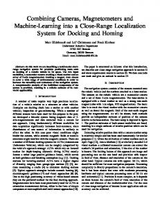
ASIC in CMOS technology designed for feedback flux induction sensor has been proposed by Rhouni et al. (2010). This miniature electronic circuit (photography of the chip on the left part of Fig. 16), is based on a differential input stage with big size input transistors (MP0 and MP1 on Fig. 16) which allow to reduce strongly the low frequency noise (1/f corner at 10Hz) usually encountered in MOS transistor. √ √ The input noise parameters of this circuit are: en = 4nV/ Hz and in < 20 f A/ Hz,close to the best amplifier while the size of the chip is only 2mm × 2mm.

62 18


Fig. 16. Design of a feedback flux amplifier ASIC (Fig. on the √ top : schematic of the ASIC circuit, Fig. on the left side: input noise measurement in nV/ Hz, Fig. on the right : photography of the chip)

4. Conclusion The method presented in this chapter to modelize the induction sensor is based on basic knowledges that can be used to study other types of sensors: elektrokinetics model, noise contributions that must be inventoriated, the computation of the sensitivity... The analytical modelling helps the beginner to become familiar with the sensor and also to manipulate general principles. Even if new technologies can offer excellent performances, in many applications induction sensors remain the best way to achieve AC magnetic field measurements. They will continue to play a role both as induction sensor and combined with other technologies Macedo et al. (2011). One can notice that in some applications, induction sensors have been replaced by other kinds of sensors, like the well known example of Giant MagnetoResistance which have replace coil in the read head of hard disks. Another example is the replacement of the pick-up coil function (like magnetoresistance in squid Pannetier et al. (2004) but also in fluxgates). When the sensitivity does matter the induction sensors still remains an efficient solution. Induction sensors is maybe not the futur of magnetometers but a stone to build this futur.


63 19

5. References (n.d.a). (n.d.b). Aharoni, A. (1998). Demagnetizing factors for rectangular ferromagnetic prisms, Journal of Applied Physics Vol. 83(6): 3432–3434. Bozorth, R. & Chapin, D. (1942). Demagnetizing factors of rods, Journal of Applied Physics Vol. 13: 320–327. Cavoit, C. (2006). Magnetic measurements in the range of 0.1-50mhz, Review of Scientific Instruments Vol. 77. Chen, D., Pardo, E. & Sanchez, A. (2006). Fluxmetric and magnetometric demagnetizing factors for cylinders, Journal of Magnetism and Magnetic Materials Vol. 306(1): 351–357. Coillot, C., Moutoussamy, J., Lebourgeois, R., Ruocco, S. & Chanteur, G. (2010). Principle and performance of a dual-band search coil magnetometer : A new instrument to investigate fluctuating magnetic fields in space, IEEE Sensors Journal Vol. 10(2): 255–260. Coillot, C., Moutoussamy, J., Leroy, P., Chanteur, G. & Roux, A. (2007). Improvements of the design of search coil magnetometer for space experiments, Sensor Letters Vol. 5: 1–4. Dupuis, J. (2005). Induction magnetometer, us patent 2005 0156601 a1. Ferrieux, J.-P. & Forest, F. (1999). Alimentations a decoupage - convertisseurs a resonance, DUNOD. Grosz, A., Paperno, E., Amrus, S. & Zadov, B. (2011). A three-axial search coil magnetometer optimized for small size, low power and low frequencies, IEEE Sensors Journal Vol. 11(4): 1088–1094. Grosz, A., Paperno, E., Amrusi, S. & Liverts, E. (2010). Integration of the electronics and batteries inside the hollow core of a search coi, Journal of App. Phys. Vol. 107. Hayakawa, M. (2007). Monitoring of ulf (ultra-low-frequency) geomagnetic variations associated with earthquake, Sensors Vol.7: 1108–1122. Lebourgeois, R., Fur, C. L., Labeyrie, M. & Ganne, J.-P. (1996). Permeability mechanisms in high frequency polycrystalline ferrites, Journal of Magnetism and Magnetic Materials 160(1-3): 329–332. Lichtenberger, J., Ferencz, C., Bodnar, L., Hamar, D. & Steinbach, P. (2008). Automatic whistler detector and analyzer system, Journal of Geophysical Research Vol. 113. Lukoschus, D. (1979). Optimization theory for induction-coil magnetometers at higher frequencies, IEEE Transactions on Geoscience electronics GE-17(3): 56–63. Macedo, R., Cardoso, F. A., Cardoso, S., Freitas, P. P., Germano, J. & Piedade, M. S. (2011). Self-powered, hybrid antenna-magnetoresistive sensor for magnetic field detection, App. Phys. Lett. Vol. 98(10). Moutoussamy, J. (2009). Ph. D. Dissertation, Nouvelles solutions de capteurs a effet de magnetoimpedance geante : Principe, Modelisation et Performances., Ecole Normale Superieure de Cachan. Osborn, J. (1945). Demagnetizing factors of the general ellipsoids, Physical Review Vol. 7(No. 0): 351–357. Pannetier, M., Fermon, C., le Goff, G., Simola, J. & Kerr, E. (2004). Femtotesla magnetic field measurement with magnetoresistive sensors, Science (304). Pfaffling, A. (2007). Helicopter electromagnetic sea ice thickness estimation: An induction method in the centimetre scale, Reports on Polar and Marine Research 553. Popovic, R., Randjelovic, Z. & Manic, D. (2001). Integrated hall-effect magnetic sensors, Sensors and Actuators A Vol. 91: 46–50.

64 20


Prance, R., Clark, T. & Prance, H. (2000). Ultra low noise induction magnetometer for variable temperature operation, Sensors and Actuators A: Physical Vol. 85(1-3): 361–364. Rhouni, A., Sou, G., Leroy, P. & Coillot, C. (2010). A very low 1/f noise asic preamplifier for high sensitivity search-coil magnetometers, Proceedings of EMSA’10 Conference, Bodrum (Turkey). Ripka, P. (2008). Inductive distance sensor for biomedical applications, Proceedings of IEEE SENSORS Conference, IEEE, pp. 1230–1232. Roux, A., Le Contel, O., Robert, P., Coillot, C., Bouabdellah, A., de la Porte, B., Alison, D., Ruocco, S. & Vassal, M. (2008). The search coil magnetometer for themis, Space Science Review Vol. 141: 265– 275. Seran, H.-C. & Fergeau, P. (2005). An optimized low frequency three axis search coil for space research, Review of Scientific Instruments Vol. 76: 46–50. Tumanski, S. (2007). Induction coil sensors - a review, Meas. Sci. Technol Vol. 18: R31–R46.

Induction Magnetometers Principle, Modeling and ...

Induction Magnetometers Principle, Modeling and ...

Suggest Documents