Jan 21, 2008 - For arbitrary continuous failure time and repair time distributions, we study the prob- ... Under these assumptions, the limiting availability A, which is the probability that ... Suppose that X1,X2,...,Xn is a random sample of lifetimes with .... estimator ËAbb of A is based on another resampling scheme which.
Inference on limiting availability of a one-unit repairable system by Fang Li and Jyotirmoy Sarkar PR # 08-01
This manuscript and other can be obtained via the World Wide Web from www.math.iupui.edu
January 21, 2008
1
Inference on limiting availability of a one-unit repairable system Fang Li and Jyotirmoy Sarkar Department of Mathematical Sciences, Indiana University Purdue University Indianapolis, 402 N Blackford Street, Indianapolis, IN 46202-3216, USA
Abstract We consider a one-unit repairable system under continuous monitoring and a perfect repair policy, with instantaneous commencement of repair and installation to operation. For arbitrary continuous failure time and repair time distributions, we study the problems of point estimation, one-sided confidence interval estimation and hypothesis testing for the limiting availability, based on a random sample of failure and repair times. MSC: primary 90B25; secondary 62N05 Keywords: Continuous monitoring; Perfect repair; Mean time to failure; Mean time to repair; Key renewal theorem; Slutsky’s theorem; Bias correction; Jackknife; Bootstrap estimation; Acceleration; One-sided confidence interval; One-sided test
1.
Introduction We consider a one-unit repairable system under continuous monitoring. In the begin-
ning, the system is put on operation, and as soon as it fails it goes to a repair facility for repair (this is called instantaneous commencement of repair). We assume that repair takes a random amount of time, after which the unit is restored back to a level equivalent to a new unit (this is called the perfect repair policy). Then it is immediately put on operation (this is called instantaneous installation). Thus, the system alternates between on and off states according as it remains operational or undergoes repair. As a benchmark to evaluate the long-term performance of a repairable system, one
1
often considers the limiting average availability Aav :=
MTTF , MTTF + MTTR
(1.1)
where MTTF stands for mean time to failure and MTTR stands for mean time to repair. Thus, Aav equals the limiting expected proportion of time the system is up. For an account on the subject see Barlow and Proschan (1975, p. 206). We assume all lifetimes are independent and identically distributed (IID) with an absolutely continuous cumulative distribution function (CDF) F (with density function f ), while all repair times are IID with an absolutely continuous CDF G (with density function g). Furthermore, the lifetimes and the repair times are stochastically independent. Under these assumptions, the limiting availability A, which is the probability that the system will be found in a functioning state much later in future, exists and, by the Key Renewal Theorem, we have A = Aav =
µF , µF + µG
(1.2)
where µF is the mean time to failure under CDF F , and µG is the mean time to repair under CDF G. See, for example, Høyland and Rausand (1994, p. 224) and Ross (1996, p. 115). In most practical applications, however, F and G are unknown. Hence, A is unknown. We consider the problem of statistical inference on A based on two independent random samples of equal size n from F and G respectively. In the literature, there has been many papers over the last two decades studying the statistical inference on A for specific lifetime and repair time distributions. See Ananda (2003), Chandrasekjar, et. al. (2004) and the references therein. In this paper, we present a comprehensive study of point estimation, confidence interval estimation and hypothesis testing on A in a non-parametric setting with fixed samples. In the non-parametric setting with arbitrary lifetime and repair time distributions, Sen and Bhattacharjee (1986) correctly point out that the natural estimator of A, given by its sample version, may not be strictly unbiased, and therefore they use a jackknife estimator to reduce the effective bias. In this paper, we additionally present several bootstrap methods to correct the bias. Sen and Bhattacharjee (1986) also point out that a fixed sample level α test may not achieve a specified power against a specified 2
alternative, or the width of a specified (1 − α) level confidence interval may not have prefixed width. Hence, they developed sequential methods of confidence interval estimation and testing procedures. In the fixed sample set up, Lim, et. al. (2004) compares the bootstrap methods proposed in DiCiccio and Efron (1996) to produce confidence intervals for A. However, none of the proposed bootstraps come out as a clear winner. In this paper, we consider another bootstrap method, the ratio bootstrap-t, and exhibit its superiority over those considered in Lim, et. al. (2004). ˆ given by the ratio of sample In Section 2, we show that the natural estimator A, mean lifetime to the total of sample mean lifetime and sample mean repair time, is consistent and asymptotically normal. However, for small to moderate sample sizes the natural estimator is biased and skewed to the left, and therefore is not useful for statistical inference in most ordinary situations. In Section 3, we exhibit that the bias in Aˆ is corrected by each of the two jackknife estimators: ordinary and infinitesimal, and three bootstrap estimators: natural, centered and balanced. In Section 4, we use several bootstrap based techniques to construct improved confidence intervals, and in Section 5 we carry out the corresponding hypothesis tests for A. We compare the performance of each inference procedure in a simulation set up using tables and graphs. The ratio bootstrap-t emerges as the best method for constructing confidence intervals and carrying out hypotheses tests for small to moderate sample sizes. Section 6 provides a summary and some concluding remarks.
2.
The natural estimator of A Suppose that X1 , X2 , . . . , Xn is a random sample of lifetimes with common CDF F
and Y1 , Y2 , . . . , Yn is a random sample of repair times with common CDF G. Assume ¯ and Y¯ denote the that the two random samples are stochastically independent. Let X 2 sample means, and SX and SY2 denote the sample variances. By Khintchine’s strong law ¯ (Y¯ ) is a strongly consistent estimator of µF (µG ). Hence, the natural of large numbers X
estimator ¯ X Aˆ = ¯ ¯ X +Y 3
(2.1)
is a strongly consistent estimator of A. Moreover, since Aˆ is bounded (between 0 and ˆ converges to A as n → ∞. Thus, Aˆ is asymptotically unbiased. 1), E[A] Only in the special case of exponential lifetimes and exponential repair times, one ˆ However, F and G are can derive the exact distribution of the natural estimator A. usually unknown. Hence, the exact distribution of Aˆ can not be derived. Nonetheless, it is straight-forward to establish the asymptotic normality of Aˆ using the central limit theorem and Slutsky’s theorem. Note that ¾ ½ ¯ √ √ µ X F n(Aˆ − A) = n ¯ ¯ − µF + µG X +Y √ ¯ n [µG (X − µF ) − µF (Y¯ − µG )] = ¯ + Y¯ ) (µF + µG )(X
(2.2)
converges in distribution to N (0, σ 2 ) where σ2 =
2 µ2F σG + µ2G σF2 . (µF + µG )4
Furthermore, since a strongly consistent estimator of σ 2 is given by ¯ 2 S 2 + Y¯ 2 S 2 X Y X σ ˆ2 = , 4 ¯ ¯ (X + Y )
(2.3)
(2.4)
Aˆ is asymptotically normal with approximate variance σ ˆ 2 /n. However, as pointed out by Sen and Bhattacharjee (1986, p. 284), in view of the fact that Aˆ is not a linear function of µF and µG (rather a ratio involving them), the natural estimator may not be strictly unbiased (although it is asymptotically unbiased). In our simulation study, we exhibit the bias of Aˆ even for moderately large sample sizes. See the ˆ A-column in Table 1. Furthermore, while Aˆ is asymptotically normal, the convergence to normality is rather slow, as exhibited in Figure 1. Therefore, for small to moderate sample sizes, confidence interval estimates and hypothesis testing based on asymptotic normality of Aˆ perform poorly in terms of lack of proper coverage and inaccurate level of test respectively, as exhibited in Table 2 and Figure 3 .
3.
Jackknife and bootstrap estimators of A In this Section, we apply different resampling schemes to construct the standard
jackknife, the infinitesimal jackknife, the natural bootstrap, the centered bootstrap and 4
the balanced bootstrap estimators of A in order to effectively reduce (but we cannot ˆ completely eliminate) the bias of the natural estimator A.
3..1
Jackknife estimators of A
¯ (i) and Y¯ (i) denote the sample means that are obtained when For i = 1, · · · , n, let X (Xi , Yi ) is omitted from the original sample. As in Sen and Bhattacharjee (1986, p. 286), we define the jackknife estimator of A and its variance estimator as n ¯ (i) n − 1 X ˆ ˆ(i) X AˆJ = Aˆ + (A − A ) with Aˆ(i) = ¯ (i) ¯ (i) , n i=1 X +Y ) ( 2 n n X X 1 (j) 2 (i) . Aˆ sJ = (n − 1) Aˆ − n j=1 i=1
(3.1)
(3.2)
The infinitesimal jackknife estimator (see Efron (1979, pp. 12-14) and Jaeckel, 1972) of A, which corrects the bias of Aˆ through a ratio (see some details in Subsection 4.4), and its variance estimator are given by " ( n µ ¶µ ¶ X ¶2 )#−1 n µ X Xi 1 X + Y X + Y i i i i AˆIJ = Aˆ 1 − 2 (3.3) ¯ −1 ¯ + Y¯ − 1 − ¯ + Y¯ − 1 n X X X i=1 i=1 ¸2 n · 2 X ˆ AIJ Xi Xi + Yi (3.4) s2IJ = 2 ¯ − X ¯ + Y¯ . n i=1 X
3..2
Bootstrap estimators of A
Let (X1∗1 , . . . , Xn∗1 ), . . ., (X1∗B , . . . , Xn∗B ) and (Y1∗1 , . . . , Yn∗1 ), . . ., (Y1∗B , . . . , Yn∗B ) denote B independent bootstrap samples chosen at random with replacement from the original ¯ ∗k and Y¯ ∗k , samples (X1 , . . . , Xn ) and (Y1 , . . . , Yn ) respectively. For k = 1, . . . , B let X denote the corresponding means of those independent resamples and let PB ¯ ∗k ¯ ∗k X X ∗+ ∗k ˆ ˆ . and A = PB k=1 A = ¯ ∗k ¯ ∗k ¯ ∗k + Y¯ ∗k ) X +Y (X
(3.5)
k=1
Note that Aˆ∗+ is equivalent to a centered Aˆ∗k obtained by pooling all B independent resamples together as one big resample of size Bn. Following Efron (1990), we define
5
the natural bootstrap and centered bootstrap estimators of A as à ! B B X 1 1 X ˆ∗k Aˆnb = Aˆ − Aˆ∗k − Aˆ = 2 Aˆ − A , B k=1 B k=1 à ! B B X 1 1 X ˆ∗k ∗+ ∗k ∗+ ˆ ˆ ˆ ˆ ˆ ˆ Acb = A − A −A =A+A − A . B k=1 B k=1
(3.6) (3.7)
The balanced bootstrap estimator Aˆbb of A is based on another resampling scheme which ensures that each of X1 , . . . , Xn and each of Y1 , . . . , Yn appears exactly B times when the B resamples are pooled together. The balanced bootstrap sample is easily obtained as follows: First pool B copies of the original X-sample together, then take a random permutation of elements of the pooled sample, and finally separate them into B blocks of n elements. Do the same with the Y-sample. Clearly, with this sampling scheme, ˆ which implies that Aˆnb = Aˆcb , and the common estimator in this case is Aˆ∗+ = A, denoted by Aˆbb .
3..3
Comparing various estimators of Aˆ
We conduct a Monte Carlo simulation study to compare the natural estimator Aˆ and the above-mentioned five bias-corrected estimators of A in terms of their bias and standard deviation. For the simulation, we choose a Weibull lifetime distribution with different values of the shape parameter b and corresponding value of the scale parameter so that the mean lifetime becomes 10, and we choose an exponential repair time with mean 1. Hence, the limiting availability is A = 10/(10 + 1) = .9091 for each lifetime distribution. We consider three values of the shape parameter of the lifetime distribution: b = 0.5, 1 and 2; representing decreasing, constant and increasing failure rates respectively. We also consider three sample sizes: n = 20, 60 and 100, to represent small, moderate and large samples. We use B = 1000 bootstrap samples. Also, each computation is repeated 1000 times. Figure 1 depicts the densities of the natural estimator Aˆ based on samples of size n = 60, under the simulation set up. Note the bias and left skewness of the densities, which render the use of Aˆ inaccurate for construction of confidence interval and for hypothesis testing. 6
0 5 10 15 20 25 30 35 0.80
0.85
0.90
0.95
Figure 1: Simulated densities of Aˆ with n = 60 and b = .5 (——), b = 1 (- - -) and b = 2 (. . . . . .).
Table 1 shows the mean departure from the true value A = .9091 and the standard deviation (in parenthesis) of 1000 replicates of various estimators. As anticipated, both bias and standard deviation of each estimator decrease with increase in sample size. The bias of Aˆ is effectively reduced by each of the five proposed estimators. The standard jackknife estimator AˆJ performed the best in bias reduction for small sample size n = 20. For moderate to large sample sizes, all five proposed bias-corrected estimators performed equally well. The simulated standard deviations of all five bias-corrected estimators are ˆ except for the natural bootstrap almost the same as that of the natural estimator A, estimator Aˆnb , which has a slightly larger standard deviation. This is reflective of the fact that the main purpose of the proposed bias-corrected estimators is to reduce the bias of Aˆ without changing the corresponding variances appreciably.
4.
Confidence intervals In this section, we construct (1 − α) level left-sided confidence intervals for the lim-
iting availability of a system with unknown lifetime and repair time distributions. The reason for considering only left-sided confidence intervals is that in case the true limiting 7
Table 1: Bias and standard deviation of various estimators of A. b
n
Aˆ
AˆJ
AˆIJ
Aˆnb
Aˆcb
Aˆbb
.5
20
-0.0185
-0.0006
-0.0068
-0.0022
-0.0049
-0.0046
(0.0528)
(0.0555)
(0.0517)
(0.0610)
(0.0532)
(0.0530)
-0.0056
0.0004
-0.0006
0.0006
-0.0005
-0.0004
(0.0274)
(0.0275)
(0.0272)
(0.0313)
(0.0273)
(0.0273)
-0.0041
-0.0004
-0.0008
0.0008
-0.0008
-0.0007
(0.0206)
(0.0206)
(0.0205)
(0.0244)
(0.0205)
(0.0205)
-0.0039
-0.0003
-0.0008
0.0007
-0.0007
-0.0007
(0.0274)
(0.0268)
(0.0268)
(0.0307)
(0.0269)
(0.0268)
-0.0016
-0.0005
-0.0005
0.0002
-0.0005
-0.0005
(0.0157)
(0.0156)
(0.0156)
(0.0177)
(0.0156)
(0.0156)
-0.0009
-0.0002
-0.0002
-0.0001
-0.0002
-0.0002
(0.0119)
(0.0118)
(0.0118)
(0.0135)
(0.0118)
(0.0118)
-0.0007
-0.00001
-0.00006
-0.00005
-0.00006
-0.00005
(0.0215)
(0.0215)
(0.0215)
(0.0252)
(0.0215)
(0.0215)
0.0003
0.0005
0.0005
0.0005
0.0005
0.0005
(0.0124)
(0.0124)
(0.0124)
(0.0143)
(0.0124)
(0.0124)
-0.0001
-0.00001
-0.00002
-0.00002
-0.00002
-0.00002
(0.0092)
(0.0092)
(0.0092)
(0.0106)
(0.0092)
(0.0092)
60 100 1
20 60 100
2
20 60 100
availability exceeds the upper bound there is no concern by the system user. Therefore, our objective is to obtain the lower bound of the confidence interval (the upper bound being 1 always). Since the natural estimator Aˆ is biased and skewed to the left, the standard lower confidence bound (LCB) σ ˆ Aˆstd [α] = Aˆ − z1−α √ , n
(4.1)
where z1−α is the (1 − α)-th quantile of a standard normal distribution and σ ˆ is given in (2.4), is not accurate in the sense that (Aˆstd [α], 1] does not achieve the desired coverage probability of 1 − α. 8
To improve the accuracy of the standard LCB, we use several bootstrap methods: percentile bootstrap (PB), bias-corrected and accelerated (BCa) bootstrap, bootstrap-t (Bt) and ratio bootstrap-t (RBt). Throughout the paper, by the α-th quantile of a set of real numbers {a1 , a2 , . . . , aB } we mean the average of the bαBc-th and the (bαBc + 1)-st order statistics, where bxc denotes the largest integer not exceeding x.
4..1
Percentile bootstrap interval
The PB interval is the simplest to motivate and is very easy to implement. See Efron and Tibshirani (1993). Let GAˆ∗ represent the empirical CDF of the bootstrap estimates {Aˆ∗k : 1 ≤ k ≤ B} of Aˆ given in (3.5). Then the lower bound of the (1 − α) left-sided PB interval is given by AˆP [α] = G−1 ˆ∗ (α) A
(4.2)
which is the α-th quantile of GAˆ∗ . Hall (1988) showed that the PB confidence intervals are only first-order accurate. That is, √ P (A ≤ AˆP [α]) = α + O(1/ n).
4..2
BCa bootstrap interval
Diciccio and Efron (1996, pp. 191-195) defines the LCB of a (1 − α) one-sided BCa interval for A, as · µ −1 ˆ ABCa [α; z0 , a] = GAˆ∗ Φ z0 +
z0 + zα 1 − a(z0 + zα )
¶¸ ,
(4.3)
where z0 is the bias correction, a is the acceleration, GAˆ∗ is the empirical CDF of the B bootstrap estimates {Aˆ∗k : 1 ≤ k ≤ B} of Aˆ and Φ is the CDF of a standard normal variate. Note that the BCa bootstrap is a generalization of the PB method in the sense that when z0 = 0 and a = 0, the BCa LCB reduces to the PB LCB. However, z0 and a are unknown. Therefore, the BCa method additionally requires estimation of z0 and a. Indeed, Φ(z0 ) = P {Aˆ < A}, and so à ! B X 1 ˆ . zˆ0 = Φ−1 I{Aˆ∗k < A} B k=1 9
Thus zˆ0 can be thought of as the number of normal units by which Aˆ differs from the median of {Aˆ∗k : 1 ≤ k ≤ B}. Interpretation and estimation of a are relatively more difficult. See DiCiccio and Efron (1996) for a detailed explanation. In short, a is the rate of change of standard deviation of Aˆ on the normalized scale. Because of its relation to Fisher’s score function, one way to estimate a is to use Pn
a ˆ=
6
ˆ¯(·) − Aˆ(i) )3 i=1 (A , P ¯ [ ni=1 (Aˆ(·) − Aˆ(i) )2 ]3/2
¯ (i) X with Aˆ(i) = ¯ (i) ¯ (i) X +Y
n
1 X ˆ(j) ¯ and Aˆ(·) = A , n j=1
√ where Aˆ(i) is the jackknife estimator of A. Thus, a ˆ is n/6 times the skewness of {Aˆ(i) : 1 ≤ i ≤ n}. The BCa LCB is given by AˆBCa [α] = AˆBCa [α; zˆ0 , a ˆ]. DiCiccio and Efron (1996) showed that the BCa one-sided confidence interval (AˆBCa [α], 1] is second-order accurate. That is, P (A ≤ AˆBCa [α]) = α + O(1/n).
4..3
Bt interval
The Bt confidence interval is conceptually simpler to describe than the BCa confidence interval and it also has the second-order accuracy property. See Hall (1988) and DiCiccio and Efron (1996, pp. 199-200). By analogy to Student’s t-statistics, we define
T =
Aˆ − A , σ ˆAˆ
(4.4)
ˆ The LCB of an (1 − α) level left-sided where σ ˆAˆ is an estimated standard deviation of A. confidence interval for A then is Aˆ − T1−α σ ˆAˆ ,
(4.5)
where T1−α is the (1 − α)-th quantile of T . However, the T -quantiles are unknown in most situations. The idea of the Bt method is to compute σ ˆAˆ and the quantiles of T by bootstrapping. Recall that Aˆ∗1 , . . . , Aˆ∗B are
10
ˆ Therefore, B bootstrap estimates of A. σ ˆAˆ =
1 B − 1
B X k=1
Ã
B 1 X ˆ∗l ∗k ˆ A − A B l=1
!2 1/2
.
(4.6)
Likewise, the standard deviation σAˆ∗k of each Aˆ∗k may be estimated by σ ˆAˆ∗k using a second level nested bootstrap resample. To be more specific, from (X1∗k , . . . , Xn∗k ) and (Y1∗k , . . . , Yn∗k ) we generate M second level nested bootstrap resamples (X1∗k,1 , . . . , Xn∗k,1 ), . . ., (X1∗k,M , . . . , Xn∗k,M ) and (Y1∗k,1 , . . . , Yn∗k,1 ), . . ., (Y1∗k,M , . . . , Yn∗k,M ). We take M = 30 in our simulation study (as recommended by Efron and Tibshirani, 1986). Then we compute σ ˆAˆ∗k =
M X
Ã
1 1 Aˆ∗k,m − M − 1 m=1 M
M X
Aˆ∗k,m
m=1
!2 1/2
,
¯ ∗k,m X Aˆ∗k,m = ¯ ∗k,m ¯ ∗k,m . (4.7) X +Y
Then we obtain B bootstrap replicates of T in (4.4) as T ∗k =
Aˆ∗k − Aˆ , σ ˆAˆ∗k
k = 1, . . . , B.
(4.8)
T1−α is estimated by the (1 − α)-th quantile of {T ∗1 , . . . , T ∗B }, and the (1 − α) level Bt LCB for A is given by AˆBt [α] = Aˆ − Tˆ1−α σ ˆAˆ .
4..4
(4.9)
Ratio Bt interval
For the Bt method we used (1 − α)-th quantile of T given in (4.4). But this T is biased. The RBt method corrects this bias via a ratio as described below. The RBt interval also is second-order accurate just as the BCa and the Bt intervals are, though it is conceptually as well as computationally simpler than the other two. h i ˆ Let ρ = E A/A and let τ˜ be a consistent estimator of the standard deviation of ˆ A/A. We modify the T in (4.4) as TBC =
ˆ −ρ A/A . τ˜ 11
(4.10)
The LCB of (1 − α) level left-sided RBt interval for A is then given by AˆRBt [α; ρ, τ˜] =
Aˆ ρ + TBC,1−α τ˜
,
(4.11)
where TBC,1−α is the (1 − α)-th quantile of TBC . However, ρ and the TBC -quantiles are unknown in most situations, and they have to be estimated. Let ρ∗ be the expectation and τ˜∗ be the standard deviation of Aˆ∗k /Aˆ under ˆ of {Yi : i = 1, . . . , n}. Efron (1979, the empirical CDFs Fˆ of {Xi : i = 1, . . . , n} and G pp. 12-14) showed that, by expanding Aˆ∗k /Aˆ in a Taylor series, we can approximate ρ∗ and τ˜∗ as ρ∗ τ˜∗
( n µ ¶µ ¶ X ¶2 ) n µ X Xi 1 X + Y X + Y . i i i i = ρ∗1 := 1 − 2 , ¯ −1 ¯ + Y¯ − 1 − ¯ + Y¯ − 1 n X X X i=1 i=1 ( ¸2 )1/2 n · 1 X Xi Xi + Yi . ∗ = τ˜1 := . (4.12) ¯ − X ¯ + Y¯ n2 i=1 X
Therefore, we can use ρ∗1 and τ˜1∗ as the bootstrap estimates of ρ and τ˜ respectively. To estimate the TBC -quantile, we construct bootstrap replicates of TBC in (4.10). Let ρ∗k be the expectation and τ˜∗k be the standard deviation of Aˆ∗k /Aˆ under F and G. As above, ρ∗k and τ˜∗k have the following bootstrap estimators
ρ∗k 1 τ˜1∗k
( n µ ¶ µ ∗k ¶ X ¶2 ) n µ ∗k Xi + Yi∗k Xi + Yi∗k 1 X Xi∗k := 1 − 2 , ¯ ∗k − 1 ¯ ∗k + Y¯ ∗k − 1 − ¯ ∗k + Y¯ ∗k − 1 n X X X i=1 i=1 ( )1/2 · ¸ n 2 1 X Xi∗k Xi∗k + Yi∗k := . (4.13) ¯ ∗k − X ¯ ∗k + Y¯ ∗k n2 X i=1
We compute the B bootstrap replicates of TBC in (4.10) as ∗k TBC
=
ˆ∗k A ˆ A
− ρ∗k 1 τ˜1∗k
,
k = 1, 2, . . . , B
(4.14)
∗1 ∗B and estimate the TBC,1−α by the (1 − α)-th quantile of {TBC , . . . , TBC }. Finally, the LCB
of the (1 − α) level left-sided RBt interval for A is given by AˆRBt [α] = AˆRBt [α; ρ∗1 , τ˜1∗ ] = 12
Aˆ ρ∗1 + TˆBC,1−α τ˜1∗
.
(4.15)
12 10 8 6 4 2 0
0.75
0.80
0.85
0.90
0.95
Figure 2: Densities of the various 95% LCBs when b = 0.5 and n = 60: Aˆstd [.05] (——), AˆP [.05] (− − −), AˆBCa [.05] (. . . . . .), AˆBt [.05] (−− −−) and AˆRBt [.05] (− · −). Indeed, one may wish to construct a bias corrected bootstrap estimator of A as follows Aˆ AˆBC = ∗ . ρ1
(4.16)
This bias corrected estimator of A in (4.16) turns out to be the same as the infinitesimal jackknife estimator of A given in (3.3). Likewise, τ˜1∗ of (4.12) is both the bootstrap ˆ estimator and the infinitesimal jackknife estimator of the standard deviation of A/A. Not only is the RBt interval a bias corrected one, but also it is easier to compute since it avoids the second level nested bootstrap resamplings.
4..5
Comparing various confidence interval estimators of Aˆ
Under the same simulation set up as in Subsection 3.3, we now compare the various confidence interval estimators in terms of the distributions of the LCBs and the coverage probabilities. Figure 2 gives the density curves of the 1000 simulated estimates of these various 95% LCBs when b = .5 and n = 60. The figure shows that all bootstrap LCBs are stochastically to the left of Aˆstd [.05], which has a coverage probability smaller than the nominated value of .95. The distributions of AˆBCa [.05] and AˆRBt [.05] are very similar with coverage probabilities close to 95%. However, the distributions of AˆBt [.05] and AˆP [.05] shift further left resulting in coverage probabilities in excess of 95%. 13
Table 2 gives the simulated coverage probabilities of the various left-sided 95% confidence intervals. An asterix indicates a statistically significant difference based on a two-sided .05-level binomial test, since each confidence interval includes A = 10/11 with a 95% probability. The table shows that all bootstrap intervals provide more accurate coverage probabilities than the standard interval. However, the PB intervals do not perform as well as the other three bootstrap intervals, attesting to the fact that the PB interval is only first-order accurate, whereas the BCa, Bt and RBt intervals are secondorder accurate. Also the RBt intervals perform better than the other bootstrap intervals in the sense that it’s simulated coverage probabilities are never significantly different from the nominated value of .95.
5.
Hypothesis testing In addition to the point and interval estimation, we also are interested in testing
hypotheses on A. Since the purpose is to demonstrate statistically that the system limiting availability exceeds the specification imposed by the user, we consider a rightsided alternative hypothesis against a left-sided null hypothesis. H0 : A ≤ A0
versus Ha : A > A0 ,
(5.1)
where A0 is the specified limiting availability. Because of its asymptotic normality, the natural estimator Aˆ leads to a standard test statistics which reject H0 at significance level α, if √
n(Aˆ − A0 )/ˆ σ > z1−α ,
or equivalently, if the left-sided confidence interval does not include A0 ; that is, Aˆstd [α] > A0 .
(5.2)
However, since Aˆ is biased and left skewed, the standard testing rule is not very accurate (does not achieve the specified significance level). The testing rule can be improved by using bootstrap intervals instead.
14
Table 2: Coverage probabilities of various left-sided 95% confidence intervals (and the corresponding attained significance levels of α = .05 tests) b
n
Aˆstd [.05]
AˆP [.05]
AˆBCa [.05]
AˆBt [.05]
AˆRBt [.05]
.5
20
0.916*
0.972*
0.953
0.966*
0.948
(0.084)
(0.028)
(0.047)
(0.034)
(0.052)
0.929*
0.969*
0.947
0.961
0.954
(0.071)
(0.031)
(0.053)
(0.039)
(0.046)
0.940
0.969*
0.953
0.964*
0.957
(0.060)
(0.031)
(0.047)
(0.036)
(0.043)
0.911*
0.945
0.940
0.959
0.955
(0.089)
(0.055)
(0.060)
(0.041)
(0.045)
0.920*
0.937*
0.939
0.954
0.946
(0.080)
(0.064)
(0.061)
(0.046)
(0.054)
0.936*
0.943
0.947
0.951
0.950
(0.064)
(0.057)
(0.053)
(0.049)
(0.050)
0.894*
0.912*
0.933*
0.947
0.942
(0.106)
(0.088)
(0.067)
(0.053)
(0.058)
0.926*
0.935*
0.946
0.952
0.948
(0.074)
(0.065)
(0.054)
(0.048)
(0.052)
0.926*
0.925*
0.943
0.950
0.945
(0.074)
(0.075)
(0.057)
(0.050)
(0.055)
60 100 1
20 60 100
2
20 60 100
Likewise, the PB, BCa, Bt, RBt intervals respectively yield the rejection regions: AˆP [α] > A0 ,
AˆBCa [α] > A0 ,
AˆBt [α] > A0 ,
AˆRBt [α] > A0 .
(5.3)
Continuing in the same simulation set up as in Subsections 3.3 and 4.5, we specify H0 : µF = 10, and consider several alternative hypotheses which assign µF = 12, 14, 16, 18. We carry out the test in (5.1) at significance level α = .05 based on n = 60 observations. Under H0 : µF = 10, Table 2 gives the simulated significance levels of the various .05level tests in the parentheses. Figure 3 depicts the simulated powers, at the chosen values A = 10/11, 12/13, 14/15, 16/17, 18/19, of these various .05-level tests. To save space, 15
0.92
0.93
0.94
0.95
0.00 0.20 0.40 0.60 0.80 1.00
Power
0.00 0.20 0.40 0.60
Power
0.91
0.91
A
0.92
0.93
0.94
0.95
A
Figure 3: Simulated powers of various tests when n = 60 and b = 0.5 (left panel) or b = 2 (right panel): std (——), P B (− − −), BCa (. . . . . .), Bt (−− −−), RBt (− · −). the case for b = 1 is omitted from the figure, as its behavior is intermediate between the cases of b = 0.5 and b = 2. The figure shows that the power of the each test increases with the true availability A. Hence, all tests are consistent. For moderate sample size, the powers of the tests based on BCa LCB and RBt LCB are close and they both have approximate size α. Their powers are slightly lower than that of the test based on the standard LCB, but this is only because the later has a size larger than α. The power of the test based on PB LCB is the smallest when b = 0.5 as it attains a much smaller size than α, but its power is a little larger than those of the other bootstrap tests when b = 2 as it does not achieve the correct α level. The power of the test based on Bt LCB is smaller for b = .5 when it undershoots the level correction, and is also smaller than those of the tests based on BCa and RBt LCB’s for b = 2 when it corrects the α level equally well as the other two. Hence, for moderate sample size it is better to use tests based on BCa LCB and RBt LCB, and between these two methods, the RBt is easier to motivate and compute.
16
6.
Summary and conclusions
In this paper, we studied a one-unit repairable system under continuous monitoring and a perfect repair policy. We considered a non-parametric set up in which the lifetime and the repair time distributions have arbitrary continuous densities. We gave a comprehensive account of statistical inference on the limiting availability of the system based on fixed sized independent samples from lifetime and repair time distributions. We exhibited the drawbacks of inference using the natural estimator, and instead advocate the use of computationally more intensive jackknife and bootstrap estimators. Regarding confidence intervals and hypotheses testing, we demonstrated the superiority of the ratio bootstrap-t method, which is easier to comprehend and implement than its closest competitor, the BCa bootstrap method. The ideas in this paper can be extended to incorporate censored lifetime data, or to a more general one-unit repairable system that is supported by one or more identical spare units. The details will be reported in a forthcoming paper. A more detailed measure of system performance is given by the instantaneous availability function A(t), which is the probability that the system is up at a specified time t > 0. For an excellent account on the subject see, for example, Høyland and Rausand (1994). Explicit evaluation of A(t) is often very difficult. For some examples see Sarkar and Chaudhuri (1999), Biswas and Sarkar (2000) and Sarkar and Sarkar (2000, 2001) and Biswas et. al.
(2003). Inference on A(t) for arbitrary lifetime and repair time
distributions is delegated to a future research project.
REFERENCES Ananda, MMA. (2003). Confidence intervals for steady state availability of a system with exponential operating time and lognormal repair time . Applied Mathematics and Computation, 137, 499-509. Barlow, R.E. and Proschan, F. (1975). Statistical theory of reliability and life testing. Holt, Rinehart & Winston, New York. 17
Biswas, A. and Sarkar, J. (2000). Availability of a system maintained through several imperfect repairs before a replacement or a perfect repair. Statistics & Probability Letters, 50(2), 105-114. Biswas, A. Sarkar, J. and Sarkar, S. (2003). Availability of a periodically inspected system maintained through several imperfect repairs before a perfect repair. IEEE Transactions on Reliability, 52(3), 311-318. Chandrasekjar, P. Natarajan, R. and Yadavalli, VSS. (2004). A study on a two-unit standby system with Erlangian repair time. Asia-Pacific Journal of Operational Research, 21(3), 271-277. DiCiccio, TJ. and Efron, B. (1996). Bootstrap confidence intervals. Statist. Sci. , 11, 189-228. Efron, B. (1979). Bootstrap methods: another look at the jackknife. Ann. Statist. , 7 1-26. Efron, B. (1990). More efficient bootstrap computations. J. Amer. Statist. Assoc. , 85 79-89. Efron, B. and Tibshirani, R. (1986). Bootstrap measures for standard errors, confidence intervals, and other measures of statistical accuracy. Statist. Sci. , 1, 54-77. Efron, B. and Tibshirani, R. (1993). An introduction to the bootstrap. Chapman and Hall, New York. Hall.
P. (1988).
Theoretical comparison of bootstrap confidence intervals.
Ann.
Statist., 16 927-985. Høyland, A. and Rausand, M. (1994). System reliability theory. Wiley, New York. Jaeckel, L. (1972). The infinitesimal jackknife. Bell Laboratories Memorandum #MM 72-1225-11. Lim, JH. Shin, SW. Kim, DK. and Park, DH. (2004). Bootstrap confidence intervals for steady-state availability. Asia-Pacific Journal of Operational Research, 21(3), 407-419. 18
Ross, S. M. (1996). Stochastic Processes, 2 ed. Wiley & Sons, New York. Sarkar, J. and Chaudhuri, G. (1999). Availability of a system with gamma life and exponential repair time under perfect repair policy. Statistics & Probability Letters, 43, 189-196. Sarkar, J. and Sarkar, S. (2000). Availability of a periodically inspected system under perfect repair. Journal of Statistical Planning and Inference, 91, 77-90. Sarkar, J. and Sarkar, S. (2001). Availability of a periodically inspected system supported by a spare, under perfect repair or upgrade. Statistics & Probability Letters, 53(2), 207-217. Sen, PK. and Bhattacharjee, MC. (1986). Non-parametric estimators of availability under provisions of spare and repair. In: Basu, A.P. (Ed.), Reliability and Quality Control. Elsevier, Amsterdam, pp. 281-296.
19