20
Alag and Agogino
Inference Using Message Propagation and Topology Transformation in Vector Gaussian Continuous Networks Satnam Alag
Alice M. Agogino
Department of Mechanical Engineering University of California at Berkeley
Department of Mechanical Engineering University of California at Berkeley
alag@pawn. berkeley.edu
[email protected]
Abstract We extend continuous Gaussian networks - directed acyclic graphs that encode probabilistic relationships between variables - to its vector form. Vector Gaussian continuous networks consist of composite nodes representing multivariables, that take continuous values. These vector or composite nodes can represent correlations between parents, as opposed to conventional univariate nodes. We derive rules for inference in these networks based on two methods: message propagation and topology transformation. These two approaches lead to the development of algorithms, that can be implemented in either a centralized or a decentralized manner. The domain of application of these networks are monitoring and estimation problems. This new representation along with the rules for inference developed here can be used to derive current Bayesian algorithms such as the Kalman filter, and provide a rich foundation to develop new algorithms. We illustrate this process by deriving the decentralized form of the Kalman filter. This work unifies concepts from artificial intelligence and modem control theory.
1 Introduction
Monitoring and estimation problems involve estimating the state of a dynamical system using the information provided by the sensors. Estimation is the process of selecting a point from a continuous space - the best estimate or the expected value. In predicting, controlling, and estimating the state of a system it is nearly impossible to avoid some degree of uncertainty (Dean and Wellman, 1991). Probabilistic (Bayesian or belief) networks directed acyclic graphs that encode probabilistic information between variables - have been found to be useful in modeling uncertainty. Our work aims at representing this estimation process by means of graphical structures and deriving rules for inference within these networks. By using this approach one can convert the tasks associated with monitoring and estimation:
sensor validation, sensor data-fusion, and fault detection, to a problem in decision theory. The main advantage of this graphical approach is the ease with which old Bayesian algorithms such as the Kalman filter, the probabilistic data association filter, multiple model algorithms, as well as new algorithms can be represented and derived using these networks and rules for inference (Alag, 1996). Practical systems consist of variables that acquire continuous values in an operating range, e.g., the temperature of a particular component being monitored or the pressure in a chamber. Therefore, to represent these variables by means of a network structure, the nodes that are associated with these variables should be able to take continuous values. Pearl (1988) has developed an encoding scheme for representing continuous variables in a belief network, which could potentially be used for our graphical framework. However, this representation, is based on the assumption that the parents of each variable are uncorrelated. This assumption breaks down when the underlying network contains loops, when two or more nodes posses both common descendants and common ancestors, which unfortunately could occur in the class of problems that we consider. We therefore develop a different encoding scheme for representing continuous variables in a belief network. This consists of extending continuous Gaussian networks to its vector form, where each node consists of a multivariate Gaussian distribution, as opposed to each node representing a univariate Gaussian distribution. These vector or composite nodes are capable of representing dynamic systems, where parent nodes may be correlated. These vector nodes correspond to the process of clustering: a method used to handle multiply connected networks. The links between these vector nodes are now characterized by matrices. To apply these
compound networks, we need rules for inference within these graphical structures. In this paper, we carry out this task for singly connected vector Gaussian networks. The case of multiply connected networks and mixed discrete-continuous vector Gaussian
21
Inference in Vector Gaussian Continuous Networks
4) and is addressed in this paper. We will develop rules for
networks can be found in Alag (1996, Chapter not
inference using first, the method of message propagation
1 988; Driver and Morrell, 1995) and second, the method of topology transformation (Olmsted, 1984; Shachter, 1986; Rege and Agogino, 1988). These two (Pearl,
methods have been
chosen because they lead to
the
development of algorithms that can be implemented either
in a decentralized (parallel using multiple processors) or a centralized (single processor) architecture. In Section
2,
the area of continuous Gaussian networks and introduce
3 we derive rules for
inference using the method of message propagation, while in
4
Section
transformation.
we
We
develop
illustrate
rules
the
for
topology
potential
of
networks by deriving the Kalman filter in Section present concluding remarks in Section
these
5 and
6. The appendix
contains rules for multivariate normal distribution that
were used in Section message to parents.
multivariate
normal
distribution
as
a belief network,
where there is an arc from x J to x, whenever
b,1 '* 0, j < i.
This special form of belief network is commonly known as a Gaussian belief network. Readers Geiger and Heckerman
are
referred t o
(1994) for a more formal definition
of Gaussian belief networks. Pearl
(1988, Section
7
.2)
has developed an encoding
scheme for representing continuous variables in a belief
we briefly review the previous work done in
vector Gaussian networks. In Section
relationship between x, and x1• Hence, one can interpret a
3, as well as an alternate form of
network, which is based on the following assumptions2
(I) all interaction between variables
are linear
sources of uncertainty are normally distributed uncorrelated
(2) the and are
(3) the belief network is singly connected3•
Pearl ( 1988) considers a hierarchical system of continuos
random variables, like the one shown set of children variables Y,, Y2, •• Y"'
in Figure 1. Each U,. U2, . , U, and a
. . The relation between
variable X has a set of parent variables
X and its parents is given by the linear equation X= b1U1 bp2 + +b.U. + v (2-3) where b,, b2, , b, are constant coefficients representing the +
· ·
• •
2 Continuous Gaussian Belief Networks
Consider a domain x, of The joint
probability
continuous variables xl' .. , x
n
density
function
multivariate nonsingular normal distribution Pr( i
) N(x; P, x)!l27rPI-'" exp =
where
x is a
for
P"' (x- .r)
N( ·)denotes the normal pdf with argument x,
x=E[x]
are
( -±(x- x)'
• .
and
P=E[(x-xf(x-x) ]
respectively,
the
and
mean
covariance
Throughout the paper we will use the symbol
represent probability, and the symbol
N()
)c2-1)
relative contribution made by each of th e
U
the determination of the dependent variable
variables to
X and
v is a
noise term summarizing other factors affecting X v is
assumed to be normally distributed with a zero mean, an:l uncorrelated with any other noise variables.
and
matrix.
Pr
to
to represent the
normal distribution. The inverse of the covariance matrix,
p-'
is also known as the precision or the information
matrix.
This joint distribution of the random variables can also be
written as a product of conditional distributions each being an independent normal distribution\ namely Pr(x)
(
= fi Pr (x, J xl' .. , xH) i=l
J
Pr x, x l' . where
m,
.
,xH) N(x,,m, =
+ f,b,1(x1- m1 ), I I J•l
is the unconditional mean of
conditional variance of
bij
.
x,
x,,
given values for xl' .
Figure 1: A fragment of a singly-connected network showing the relationships between a continuous variable X its parent variables U,, U2, , U" and the noise v. Given the network topology, the link coefficients (b s), • •
v,)
(2-2)
v,
is the
.
, x,_,,
and
the variances
of the noise terms, and the means an:l '
(a�)
variances of the root variables - nodes with no parents -
(1988) has developed a distributed scheme for and variances of every variable in the network to account for evidential data e a set of
Pearl
updating the means
-
is a linear coefficient reflecting the strength of the 2The first two assumptions are the same as those made by
1 This presentation is similar to that of Geiger and
Heckerman, 1994.
Kenley and Shachter,
1989.
'A network in which no more than one path exists between two nodes
Alag and Agogino
22
variables whose values have been detennined precisely. The update can also be done in a manner similar to that in Shachter and Kenley (1989). However, Pearl places an additional restriction that the computation be conducted in a distributed fashion, as though each variable were managed by a separate and remote processor communicating only with processors that are adjacent to it in the network, i.e., the update is performed in a decentralized {parallel) manner. The equation relating the variable of interest to its parents replaces the conditional probability table that is required in the case where the variables are discrete. In addition, due to the assumption that the variables are normally distributed the complete distribution can be specified with the help of just two parameters: the mean and the variance. We extend these continuous Gaussian networks to their vector form. Figure 2 shows a generic form of a vector Gaussian network. Here, the variables ( U,, X,
Y)
represented X=
[x1,..
by
,x.
f
,
the
where
nodes
x,
are
vectors,
for
e.g.,
are Gaussian random variables.
one may cluster the variables into nodes in which there is no evidence, nodes with different covariance matrices, correlated variables, etc. Each clustered (vector) node can be considered as made up of another Gaussian belief network where the inter-relationship between the variables of this continuous Gaussian belief network is given by the node's covariance matrix.
3 Inference using Message Decentralized Approach
Propagation:
Consider a typical fragment of a singly connected network (Figure 2), consisting of an arbitrary node X, the set of all and the set of all X's X's parents, U children, Y
={UpU2, .. ,U,}, ;;;;{ f1 , Y2, .., Y,}. Let e
be the total evidence
obtained, e� be the evidence connected to X through its
e:
children (Y), and
be the evidence connected to X
through its parents (U). The readers are referred to Pearl (1988; Section 7.2) where the rules for propagation are derived for the scalar case as shown in the network in Figure l. To derive the inference rules for vector Gaussian networks, we will follow a procedure similar to Pearl's for the scalar case. Links in Pearl's network correspond to x=
+v
L, b1u, i
y=x+w1
(3-1)
The readers are also referred to the Appendix, which contains the rules for vector Gaussian distributions that are used in this derivation. Unlike Pearl, we consider normalizing constants for Gaussian distributions and show why they can be neglected.
Figure 2: Generic fo rm of a vector Gaussian belief
network. The arc between the variables represent the following relationship X= F, + v; Y, = H,X + w1 (2-4)
L U, Y, are ·
where U, and n.
Q
E[ ] r vv
,
and
"r.
dimension vector, F, is a
is a nr x n. matrix, V is a n. vector, , the covariance matrix for the noise term
x nu, matrix, =
nu,
H1
represents the correlation between the parent variables, is a
nr,
3.1 Belief Update Consider the general vector belief network in Figure 2. The links between the nodes correspond to
x= L, F, ·u1 i
+v
y1 = H,x+w,
(3-2)
The belief for node X is
BEL(x);;;; f(xle;,e:) = a· f(xle;)f(e�lx) = a· ;r(x)·ll(x)
n(x) !(xle;) J · J f(xie;, u,, .., u. )!( =
=
u1 u" ·
, .., u, e ; du, · ·du.
! )
U1
w1
vector. It can be easily shown that in the case of
multiple parent nodes
[ u., u2 r with
corresponding state
matrices F1, F2 respectively, one can obtain an equivalent matrix F"l•iWJIW
=
[F, 0] 0
F2
which express the augmented state vector [XI' x2
r.
using Rule 3 from the appendix, we get
(
1r(x);;;; N x;
i B,P., B,T i=l
;;;; N[x;P,.,x,.] This
procedure is known as clustering of the nodes. In general
+Q,iB,ut) i- 1
(3-3)
Inference in Vector Gaussian Continuous Networks
P.
The variance
can be interpreted
uncertainty in each of the
u,
L
(i.e.,
1=1
uncertainty in the relationship between Similarly, we now compute
of child nodes of X, let Q
=
as
"
E
-:t-
cJ)Ie7
of
the
part of this paper, we will neglect the constants.
cJ) denote the set
To prescribe how the influence of new information will
,
.,
}
u, (i.e., Q).
0 , and let
m
be
the number of elements in Q. Next, we relabel the child
nodes so that nodes Y1 through Y, correspond to the nodes -:t-
e7
with
A
Jt(x)=l.
0. If m = 0 then
A
Jt(x)=ltr (x).
For
m
'P;'Y, l '
f N(y;P,.xJN(y;P2,xfty;;;;: N(x; P, + P1,x,) f N(x;P,,y)N(y;Py,y)dy = N[ P, PY,y] '
•.
(
P. (u,) = N B, u, ; P� + Q+ f;B.P.,B;.:x,- t; B1ii1)
Combining the above two equations to update the belief in ui
N(B,u,; B,P:,�B,', B,U,...... )
x;
+
Refer to Alag (1996; Chapter 2) for detailed proofs.
l
[
r
B,P:;" B{ { B,�,,B,') (B,P,,B.') P. + Q+ �B,P,, B: ( B ,P.,�') -
=
[
B,ii;''� BJi, +(B,P..,Bn p" + Q+ �B,P.,B; =
J l
=
u,;P,
ii, + P.,Br[PA the
[t
J'(
x,-
f..B,u,
)
r B,P.,. 1 r (:X f. Btiit )J
-P.,B.'[P, +Q+ ?B,P,B; +Q+
above
HJR1-:"1H1r1
requirement by noting
x;P,-P,(P,+P,r'P,,
where again a is some constant.
8.
P,.(u;) =N (u,, P , iJ.) = N ( B,.u,; B,P.,B,r, B,U,)
P;.
l
)
u,
when
is some constant.
5.
7.
= N(x;Q+ tB1PAr·l{BJi1
7.2 Alternate Forms for Message to Parents We can simplify the belief update process for the parent node (continued from Section 3.3)
=
J
where the constant a is given by
6
9.
J
N( u,; P:', U,"w)
P,[ATP ,�'(y-B) '
N(x;P,.xJN(x;Pz,x,)=a·N
here
"' 1=1
uI
Therefore,
7 Appendix 7.1 Rules for Vector Gaussian Distribution4
)
J-· J(I N(u,, P,.ii,)· N( L,s,u,,Q,x du, · ·du.
HI
'f-B P., B: .
formula
is
A-
used
to exist. We
can
we
require
remove
this
6
=HTW'H pA- l=' k HTW'H J J I j:::d
T T, ]T H= [H,,··,H..
l
... R= HP,HT
where
is the
m
which there
R = blockdiag{ R,, .., R.,}
P�' = H7[HP,HTr H
number of children nodes of X through is evidence. But
[P. +Q+f.B,P.,B: r =H'[H(Q+ fB,P,,B: )w +RrH
Further,
P;'xA = IH7.R1-'Y', '"
j;l
HT W' HXA :.HX),
=y
N(u,:P ,u, �
•.
is
--·
)
=
=
=
HT K'y
HrK'y
[u,:P, -P,,B,'H'[H(Q+�B,P,,B:)H'+RrHB,P,, 1 , ii, P,,B; H'[ H(Q+ fB,P B� )w + R J (y- H�B,ii',)
N
+
•.
an alternate form for updating the beliefs.