Teaching Inflation Targeting: An Analysis for Intermediate Macro
Carl E. Walsh*
First draft: September 2000 This draft: July 2001
*
Professor of Economics, University of California, Santa Cruz, and Visiting Scholar,
Federal Reserve Bank of San Francisco. Mailing address: Department of Economics, SS1, University of California, Santa Cruz, CA 95064 (voice: 831-459-4082; Fax: 831459-5900; email:
[email protected]). Any opinions expressed are those of the author and not necessarily those of the Federal Reserve Bank of San Francisco or the Federal Reserve System. I would like to thank Betty Daniel and the referees for helpful suggestions and comments.
Teaching Inflation Targeting: An Analysis for Intermediate Macro
Abstract Over the last decade, many central banks have adopted polices known as inflation targeting. To prepare intermediate level macroeconomics students to think about current policy issues, it is important to provide them with an introduction to the macroeconomic implications of inflation targeting. Unfortunately, the standard aggregate demandaggregate supply frameworks commonly used to teach intermediate macroeconomics are not well suited for this task because they are expressed in terms of output and the price level and because they fail to make explicit the policy objectives of the central bank. This paper provides a simple graphical device involving the output gap and the inflation rate that overcomes these problems and that can be used to teach intermediate macroeconomics students about inflation targeting.
1. Introduction Over the last decade, many central banks have adopted monetary polices known as inflation targeting. New Zealand, the United Kingdom, Sweden, Canada, Mexico, and Israel are among the countries employing inflation targeting in the conduct of monetary policy, and the European Central Bank has been urged to follow suit (Svensson 1999). If intermediate level macroeconomics classes are to prepare students to think about current policy issues, it is important to provide them with some introduction to the implications inflation targeting has for macroeconomic behavior. Unfortunately, the standard aggregate demand—aggregate supply frameworks commonly used to teach intermediate
2
macroeconomics are not well suited for analyzing inflation targeting for two reasons. First, these frameworks are expressed in terms of output and the price level and, second, the policy objectives of the central bank are not made explicit. The purpose of this paper is to provide a simple graphical device that involves the output gap (output relative to its full-employment level) and the inflation rate and that can be used to teach intermediate macroeconomics students about inflation targeting. The framework also makes explicit the role played by the policy objectives and preferences of the central bank. In section 2, the basic framework is set out. Two relationships are employed. The first is an expectations augmented Phillips Curve derived from the assumption that prices are sticky. The second is a description of monetary policy behavior. The basic framework is consistent with recent research using models in which the central bank implements monetary policy through the use of a nominal interest rate as its policy instrument.1 The framework is used in section 3 to illustrate how the economy responds to economic disturbances under inflation targeting, and how the variability of inflation and the output gap depend on the policy preferences of the central bank. Section 4 examines the linkages between the central bank’s policy instrument, the output gap, and inflation. The analysis leads naturally to a view of policy as responding systematically to economic developments, consistent with the evidence that "most variation in monetary policy instruments is accounted for by responses of policy to the state of the economy, not by random disturbances to policy" (Sims 1998, page 933). It also highlights the role of policy objectives in affecting the way the central bank manipulates its policy instrument and in affecting the behavior of the economy. This last feature is important since central banks have, in the past, shifted the relative emphasis
3
they appear to place on inflation and other economic goals. These shifts can be analyzed in the proposed framework because the linkages between preferences, policy instruments, and equilibrium are made explicit. The framework leads to an instrument rule for the nominal interest rate that is similar to a Taylor Rule, but the construction helps to make clear why empirical policy reaction functions may find that additional factors also affect policy.2
2. The Model The model of inflation targeting has two components. The first is an expectations augmented Phillips curve. This component is a standard part of macroeconomic models that incorporate the assumption of sticky price and/or wage adjustment. The second component is a description of monetary policy, reflecting the policy maker’s preferences in trading off fluctuations in output and inflation. This second component provides a reduced form representation of the demand side of the model.3 The linkages between the instrument of monetary policy and aggregate demand are made more explicit in Section 4.
2.1 The expectations augmented Phillips Curve The Phillips Curve relates inflation π to (a) expectations of inflation πe, (b) the state of the business cycle, measured by the gap between output y and the natural rate of output yn (output at full-employment) and (c) an inflation shock e that captures any other factors affecting inflation. For convenience, let x denote the percent output gap (x = (yyn)/yn). The Phillips Curve is written as
4
(1)
π = πe + ax + e
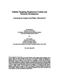
This defines a linear (for simplicity) relationship between the output gap and inflation and is shown in Figure 1 as the curve labeled PC. The intercept is equal to πe + e and the slope is a. Ignoring for the moment the shock e so that the intercept is simply πe, the PC curve in Figure 1 is drawn for an expected inflation rate of 4 percent. Equation (1) is a standard part of most macroeconomic models that are developed in intermediate level textbooks and that assume some degree of sluggish wage or price adjustment (e.g., Hall and Taylor 1997, Dornbusch and Fischer 1998, Mankiw 2000, Blanchard 1999). Recent research that has come to be labeled “New Keynesian” (Clarida, Galí, and Gertler 1999 and references found there) also includes an expectations augmented Phillips Curve, but differs from the specification in (1) in two ways. First, the expectational variable is forward-looking. When firms set prices that remain fixed for several periods into the future, they will be concerned with the future path of inflation. Second, models that derive the Phillips Curve from an explicit optimizing problem imply that the coefficient on expected future inflation should not equal 1 but should equal the subjective rate of discount. Since the latter would be close to 1 at a quarterly frequency, New Keynesian Phillips Curve often impose the restriction that the coefficient on the expected inflation term equals 1. For teaching the basics of inflation targeting, whether the expectations term in (1) represents expectations of current or of future inflation is not critical.
5
2.2 The monetary policy rule Standard macroeconomic models combine a Phillips Curve (or some other representation of the aggregate supply side of the economy) with an aggregate demand curve. This approach has two limitations. First, the usual derivation of an aggregate demand curve leads to a relationship linking the price level with the level of output or the output gap. Unfortunately, such a relationship makes it difficult to provide students with a clear analysis of inflation targeting. It will prove much more convenient and pedagogically advantageous to replace the standard aggregate demand curve with a relationship that is consistent with the demand side of the economy but which relates the output gap to the inflation rate. Second, the standard aggregate demand curve fails to make the role of monetary policy explicit. The implicit assumption is that the central bank fixes the nominal stock of money and fails to react systematically to economic developments. Such an assumption is clearly inappropriate if the point is to analyze a policy of inflation targeting. The traditional approach also makes monetary policy actions (shifts in the nominal quantity of money) appear exogenous rather than reflecting the fact that most policy actions represent endogenous reactions to the economy (Rudebusch 1998, Sims 1998). It is better to focus explicitly on the central bank’s policy choice. One approach to dealing with monetary policy in a more satisfactory manner is exemplified by the work based on “Taylor Rules” (Taylor 1993). A Taylor rule specifies how the central bank reacts to inflation and economic activity. The basic Taylor rule provides a good empirical description of Federal Reserve policy since the mid-1980s, and Clarida, Galí, and Gertler (1999) have shown that other major central banks behavior similarly. A second approach starts with the objectives of the central bank, typically
6
assumed to be the stabilization of inflation and the output gap. The central bank then sets its policy instrument to further these objectives. It will be useful to employ this second approach, but section 4 demonstrates how the policy that results is consistent with a Taylor rule. One advantage of starting from the central bank’s objectives is that it serves to highlight how changes over time in the objectives of monetary policy will result in different policy behavior. To analyze inflation targeting, assume the monetary policy authority acts systematically to minimize fluctuations of the output gap and the inflation rate around its inflation target πΤ. By systematically, I mean that the monetary authority balances the marginal costs and benefits of its policy actions—in other words, it behaves optimally, given its objectives. Assume the marginal cost to the central bank of fluctuations in either inflation or the output gap is proportional to the deviations from their respective targets of πT and zero. This is the case, for example, if the central bank’s objective is to minimize squared deviations of π and x around their targets. Let the marginal costs of output fluctuations be λx and the marginal costs of inflation fluctuations be k(π − πΤ). The parameter λ (k) is a measure of the cost of output (inflation) fluctuations as perceived by the central bank. Consider a central bank faced with a recession (x < 0) and thinking about trying to push x closer to its target of zero. Increasing x slightly, by ∆x, yields a gain of -λx∆x. There is a cost, however, since the increase in x increases inflation. The effect on inflation is, from equation (1), a∆x and the cost of this is ak(π − πΤ)∆x. Equating marginal costs and benefits yields -λx∆x = ak(π − πΤ)∆x, or
(2)
x = - (ak/λ)(π − πΤ)
7
This is the relationship between the output gap and deviations of inflation from target that is consistent with a monetary policy designed to minimize the costs of output and inflation variability. If the monetary authority could control the output gap exactly, it would always adjust policy to ensure the marginal benefits and costs balanced. In this case, equation (2) would hold exactly. More realistically, factors other than systematic monetary policy influence aggregate demand and output in ways that the monetary authority cannot forecast perfectly. In addition, policy makers may have goals beyond inflation and output gap stabilization (financial market stability for example) that would shift the relationship between the output gap and inflation given in equation (2). If u denotes the net impact on output of these additional factors (including fiscal policy), then the relationship between the output gap and inflation consistent with systematic policy becomes
(3)
x = - (ak/λ)(π − πΤ) + u
This can be rewritten as
(4)
π = πT - α(x – u)
where α = λ/ak. This equation defines a linear relationship between the output gap and inflation. Its intercept is πT + αu and its slope is α. Ignoring for the moment the disturbance term u, equation (4) is shown in Figure 1 as the curve labeled MPR (for
8
monetary policy rule). 4 In the figure, the central bank’s target rate of inflation is 2 percent. Note that the slope of the MPR curve depends on the relative importance to the monetary authority of output and inflation objectives, λ/a. An increase in the importance of output (an increase in λ) increases the slope of the MPR curve. The MPR curve is shifted by realizations of the disturbance u arising from unpredicted fluctuations in aggregate demand or from changes in monetary policy in reaction to factors other than inflation or output.
3. Analysis We can now use the PC and MPR curves to analyze the determination of the output gap and inflation, to see how the equilibrium is affected by inflation expectations and the monetary authority’s inflation target, to explore how both respond to economic shocks, and to illustrate how the volatility of output and inflation depends on the relative importance the central bank places on reducing output and inflation variability.
3.1 Equilibrium The economy’s short-run equilibrium occurs at the intersection of the PC and MPR curves. In Figure 1, this is shown as point E1. Point E1 is consistent with the Phillips Curve—at the output gap associate with E1 firms are setting prices such that the inflation rate is at the value given by E1. The equilibrium is also consistent with the behavior of the central bank. At E1, the marginal benefit of pushing output closer to the natural rate (increasing x so that is closer to zero) is just balanced by the marginal cost of
9
the additional inflation that would result from such an output expansion. As drawn in the figure, the economy’s short-run equilibrium involves a negative output gap—output is below the natural rate. This is consistent with the monetary authority’s policy choice because inflation is above the inflation target. The central bank is willing to accept a recession because it views inflation as too high. At point E1, inflation is above the central bank’s target but it is below the level expected by households and firms. Over time, as people recognize that actual inflation is less than they had expected, expected inflation will fall. This reduction in expected inflation shifts the PC curve downwards. This lowers actual inflation for each value of the output gap. With inflation lower, the marginal cost of inflation is also reduced, leading the central bank to opt for a more expansionary policy stance (how this translates into a change in the nominal interest rate is discussed in section 4 below). The short-run equilibrium moves towards lower inflation and a higher level of output (a smaller but still negative output gap), following the intersection point of the MPR curve and the shifting PC curve. Eventually, the PC curve will shift down until the inflation rate is equal to the monetary authority’s target. At this point the output gap is zero, and expected and actual inflation are both equal to the central bank’s inflation target. This is the economy’s longrun equilibrium. The adjustment of inflation expectations plays a critical role in moving the economy from a point such as E1 in Figure 1, where inflation is above target and the economy is in a recession, to a long-run equilibrium with inflation equal to its target and the output gap equal to zero.
10
The same process would operate in reverse if the initial equilibrium involved a positive output gap and inflation below the central bank’s target. In this case, actual inflation would exceed the rate expected by the public, and expected inflation would rise over time. As this rise in expected inflation increases actual inflation, the central bank tightens policy to reduce output and the output gap is reduced towards zero. The long-run equilibrium occurs where the MPR curve crosses the inflation axis, with the output gap equal to zero and actual inflation equal to the central bank’s target.
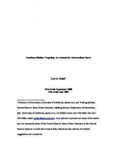
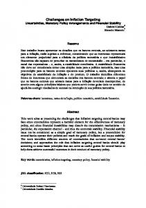
3.2 A Shift in the Inflation Target In Figure 1, the economy eventually reaches equilibrium with a zero output gap and inflation equal to πΤ. As illustrated in the figure, the target inflation rate was positive. Many central banks in recent years have been assigned the goal of price stability, and this is usually interpreted to mean the central bank should target a zero rate of inflation. Suppose a central bank that has targeting a positive inflation rate decides to reduce its target for inflation to zero. The effects of a reduction in the inflation target are shown in Figure 2. The initial equilibrium is at E0. As shown in Figure 2, the reduction in the inflation target shifts the MPR curve down from MPR1 to MPR2. The new, short-run equilibrium occurs at point E1 with some reduction in inflation and a fall in output below the natural rate (a negative output gap). From the Phillips Curve, the central bank knows it must generate a recession if it wants to reduce inflation. At point E1 in Figure 2, actual inflation is below expected inflation. The economy is in a position exactly equivalent to the one analyzed in Figure 1. As inflation
11
expectations fall, the economy eventually returns to full employment (a zero output gap) and inflation is reduced to zero, the new targeted rate.
3.3 Economic Shocks We can now reintroduce the inflation and demand shocks e and u. However, it will be useful to analyze the impact of each separately.
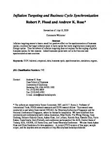
3.3a An inflation shock Suppose there is a negative inflation shock, e < 0, that temporarily lowers inflation at each value of expected inflation and output gap. From the definition of the Phillips Curve, the intercept of the PC curve is equal to πe + e, so a negative e shifts the curve down. An inflation shock has no direct effect on the MPR curve, so this curve remains unchanged. The downward shift in the PC curve leads, in the short-run, to a fall in inflation. Since this reduces the marginal cost of inflation, the central bank acts to stimulate output and the new short-run equilibrium has a positive output gap. This is illustrated in Figure 3. In subsequent periods, if e returns to zero, the PC curve returns to its original positive and inflation returns to its targeted value. The output gap also returns to zero. Both the expansion in real economic activity and the fall in inflation in response to the shock are temporary.
3.3b A demand shock A positive demand shock shifts the MPR curve to the right. At each rate of inflation, the positive shock to demand increases the output gap. The new short-run
12
equilibrium occurs at E1 in Figure 4. Because u represented unpredicted shifts in demand that the central bank could not offset, u shocks are strictly temporary in nature. On average, u equals zero, and the MPR curve returns to its original position. The economy returns to E0.
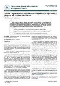
3.5 Fluctuations and the Policy Rule The slope of the MPR curve affects the relative volatility of the economy as it experiences inflation shocks. This is illustrated in Figure 5, which shows the impact of a positive inflation shock. The figure includes two alternative MPR curves with different slopes. If the economy is characterized by a steep policy curve such as MPR1, a positive inflation shock leads to a large rise in inflation and a relatively small fall in the output gap. Recall that the slope of the MPR curve is equal to α = λ/ak. A steep MPR curve occurs when the central bank places a large value on output gains (measured by λ) relative to the value placed on the cost of inflation (measured by the parameter k). In the face of an inflation shock, such a central bank acts to limit fluctuations in output, letting inflation fluctuate more instead. MPR2 represents the monetary policy rule of a central bank that is more concerned with inflation, that is, for a central bank whose ratio of λ to k is smaller. In the face of the same positive inflation shock, this central bank will try to limit the rise in inflation. As a result, it will contract output to offset most of the impact of the shock on inflation. Inflation rises less and output falls more when MPR2 characterizes policy than when MPR1 does.
13
In the face of a negative inflation shock, a central bank that is primarily concerned with inflation (a small λ relative to a and a flat MPR curve such as MPR2) offsets most of the impact of the shock on inflation, letting output rise more. The central bank more concerned with output stability (a large λ relative to a and a steep MPR curve such as MPR1) allows the shock to affect inflation more and keeps output more stable. As a consequence, over time, inflation will be more volatile and output less with a policy rule such as MPR1, while inflation will be more stable and output more volatile with a policy rule such as MPR2. The dependence of inflation and output gap volatility on the slope of the MPR curve gives rise to what John Taylor has characterized as the “new policy trade-off.” As the relative weight placed on output (λ/k) rises, the MPR curve becomes steeper. Consequently, the variance of the output gap falls while the variance of inflation increases. A central bank that places a large weight on output stability (a large λ/k) accepts more inflation variability and less output variability than a central bank with a large weight on its inflation objective would. Attempting to achieve greater inflation stability comes at the cost of increased variability in real economic activity. Placing greater stress on keeping output stable around the natural rate will lead to greater fluctuations in the inflation rate around its target rate.
4. Behind the MPR Curve In the preceding analysis, it proved convenient to leave the details of policy implementation in the background. Instead, the MPR curve simply summarized the relationship between the output gap and inflation that was consistent with optimizing
14
behavior by the central bank in balancing the marginal costs and benefits of its policy actions. Lying behind the MPR curve, however, is the monetary transmission mechanism—the linkages that connect changes in the central bank’s instruments to output and inflation outcomes. The Federal Reserve, like other major central banks throughout the world, uses a short-term nominal interest rate to implement policy. In the U.S., the Fed uses its control over non-borrowed reserves to ensure the federal funds interest rate equals the target value set by the Federal Open Market Committee (FOMC). Deviations of the funds rate from the FOMC’s target are small and short-lived. For this reason, it simplifies the analysis if one treats the nominal funds rate as if it were the direct instrument of monetary policy. The link between the funds rate and both real economic activity and inflation operates through aggregate demand. The traditional IS relation treats real aggregate demand as a decreasing function of the real rate of interest. A simple IS curve (scaled by the natural rate of output) can be written as
(5)
y/yn = y0/yn – b[i - πe] + u
where i is the nominal rate of interest. The negative coefficient on the real interest rate in the IS relationship can reflect intertemporal substitution effects on consumption as in recent new Keynesian models as well as traditional effects on investment operating through both the cost and availability of credit. The demand shock, u, was introduced earlier as the part of any aggregate demand disturbance that the central bank could not
15
foresee at the time policy was set. As such, it is assumed to be serially uncorrelated with mean zero.5 The long-run equilibrium real rate of interest is then given by
(6)
r* = (y0 – yn)/byn
Since the graphical analysis was expressed in terms of the output gap x, it is convenient to subtract one from both sides of the IS relationship to obtain
x = x0 – b[i - πe] + u
where x0 = (y0 – yn)/yn. Given the definition of r* in equation (6), one can write
(7)
x = -b[i - πe – r*] + u
In the absence of demand shocks, output will be below the natural rate (x will be negative) if the current real interest rate is above the (time varying) long-run equilibrium rate r*. Policy rules such as that proposed by Taylor (1993) express the central bank’s instrument, i, as a function of inflation and the output gap. Because both inflation and the output gap are endogenous variables, there are often several ways to express the reaction rule (Svensson and Woodford 1999). Since the graphical analysis shows the short-run equilibrium values of x and π as functions of expected inflation, the inflation target, and the realizations of the disturbances, one way to express the policy rule is to solve
16
equations (1) and (4) for x, substitute the result into (7) and solve for the value of the interest rate consistent with the short-run equilibrium. Doing so yields
i = r* + πe – (πT - πe - e)/[b(a+α)]
(8)
= iT + [1 + 1/b(a+α)] (πe - πT ) + e/b(a+α)
where iT = r* + πT is the nominal interest rate in the long-run equilibrium. The policy rule does not involve u since, by assumption, the central bank must set i prior to observing the disturbance u. The coefficient on expected inflation in (8) is greater than 1. The policy rule calls for increasing the nominal interest rate more than one-for-one whenever expected inflation rises above the central bank’s inflation target. This ensures that a rise in expected inflation leads the central bank to boost the nominal interest rate enough to raise the real rate of interest, thereby contracting the real economy. In addition, the nominal rate is fully adjusted for any changes in the central bank’s estimate of r*, the long-run equilibrium real interest rate. The nominal rate is also raised in response to a positive inflation shock. This is why a positive inflation shock reduces the output gap (see Figure 3). There are other, equivalent, ways to express the nominal interest rate that are also consistent with the equilibrium found in section 3. For example, inverting the IS curve and then using equation (4) leads to
(9)
i = r* + πe + (1/αb)[π - πT ]
17
This way of writing the interest rate rule shows that the nominal interest rate is increasing in the gap between current inflation and the inflation target. This representation is quite intuitive—if inflation exceeds the target, raise the nominal interest rate, if inflation is less than the target, lower it. In Taylor (1998), Romer (2000), and Stiglitz and Walsh (forthcoming) the demand side of the macroeconomy is represented by an aggregate demand-inflation curve that is derived from the IS curve and a monetary policy rule. Although the typical derivation is based on a Taylor rule for the nominal interest rate that assumes the central bank responds to both inflation and the output gap, the basic points can be illustrated with the simpler rule given by equation (9) in which the central bank adjusts the nominal rate in light of expected inflation and the deviation of actual inflation from target. Substituting (9) into the IS curve (7) to eliminate the nominal interest rate yields
x = -[(1/α)[π - πT ] + u
which is exactly in the form of the MPR curve assumed in section 2. One advantage of the approach used in section 2 is that it highlights the role played by the central bank’s preferences (the weights on output and inflation objectives) in affecting the slope of the MPR curve. If one starts directly with a simple Taylor-type rule, the connection between the coefficients in the rule (and ultimately in the aggregate demand-inflation) curve and policy preferences is less explicit. This also reflects the fact that equation (9) was derived
18
as an optimal instrument rule based on the assumed objective of the central bank, while a simple Taylor rule with arbitrary coefficients is generally not an optimal rule.
4. Conclusions Because so many central banks are adopting inflation targeting as a framework for conducting monetary policy, it is important to provide students taking an intermediate level macroeconomics course with a means of understanding its implications for the macroeconomy. The graphical analysis provided here does this. It uses two relationships between inflation and the output gap to determine the short-run equilibrium. The first relationship is a standard Phillips Curve. The second is a reduced form for the aggregate demand side of the economy expressed in a way that emphasizes the important role played by the central bank’s policy choice between inflation and output variability. In addition to providing a convenient framework for analyzing inflation targeting, the approach is well suited for highlighting the uncertainties associated with monetary policy. The effects of changes in the public’s expectations concerning inflation, unforecastable fluctuations in demand, and policy reactions to factors other than inflation and the output gap can all be treated within a single framework. Students can use the framework to understand how shifts in the relative weight the central bank places on its objectives will alter the volatility of inflation and output. Such shifts alter the central bank’s instrument rule as well, consistent with the empirical evidence that policy reaction functions have changed over time (see the discussion in Rudebusch 1998). As with any attempt to compress the richness of the economy into a simple graphical framework, much has been left out of the analysis. For example, by assuming
19
the central bank is concerned with stabilizing the output gap, issues of dynamic time inconsistency have been ignored.6 Instability in the MPR or PC curves, the central bank’s uncertainty about the position of the PC curve, uncertainties about the linkages between its policy instrument and aggregate demand, or uncertainties over the appropriate objectives of monetary policy all play a role in affecting the actual conduct of monetary policy. The proposed graphical presentation put forward here, however, provides an organizing framework that can help student think about issues of inflation and output stabilization.
References Clarida, R., Galí, J., and Gertler, M. 1999. The Science of Monetary Policy: A New Keynesian Perspective. Journal of Economic Literature. 37 (4): 1661-1707.
Dornbusch, R., Fischer, S., and Startz, R. 1998. Macroeconomics, 17th ed. New York, NY: Irwin McGraw-Hill.
Blanchard, O. 1999. Macroeconomics. 2d ed. Upper Saddle River, NJ: Prentice Hall.
Hall R. E., and Taylor, J. B. 1997. Macroeconomics, 5th ed. New York, NY: W.W. Norton.
King, R. G. 2000. The New IS-LM Model: Language, Logic, and Limits. Federal Reserve Bank of Richmond Quarterly Review, 86 (3): 45-103.
20
Mankiw, N. G. 2000. Macroeconomics. 4th ed. New York, NY: Worth Publishers.
Romer, D. 2000. Keynesian Macroeconomics without the LM Curve. Journal of Economic Perspectives,.14 (2): 149-169.
Rudebusch, G. D. 1998. Do Measures of Monetary Policy in a VAR Make Sense? International Economic Review. 39 (4): 907-931.
Sims, C. A. 1998. Comment on Glenn Rudebusch’s ‘Do Measures of Monetary Policy in a VAR Make Sense?’ International Economic Review. 39 (4): 933-941.
Stiglitz, J. E. and Walsh, C. E. forthcoming. Economics. 3th ed. New York, NY: W.W. Norton.
Svensson, L. E. O. and Woodford, M. 1999. Implementing Optimal Policy through Inflation-Forecast Targeting.
Taylor, J. B. 1993. Discretion versus Policy Rules in Practice. Carnegie-Rochester Conference Series on Public Policy. 39: 195-214.
Taylor, J. B. 1998. Economics. 2d ed. Boston, MA: Houghton Mifflin.
21
Walsh, C. E. 1998. The New Output-Inflation Trade-off. Federal Reserve Bank of San Francisco Economic Letter. 98 (4).
Walsh, C. E. 1998. Monetary Theory and Policy. Cambridge, MA: MIT Press.
22
FIGURE 1 Output and Inflation with Inflation Targeting Inflation (%)
8
PC
6
E1
4
π
e
Τ
π
2
0 -6
-4
-2
0
2
4
6
8
10 Output gap (%)
-2
-4 MPR
-6
23
FIGURE 2 A Shift in the Inflation Target Inflation (%)
8
6
PC
4
E0 E1
2
E2 0 -6
-4
-2
0
2
4
6
8
10 Output gap (%)
-2
-4
MPR2 MPR1
-6
24
FIGURE 3 A Temporary Inflation Shock 8 Inflation (%)
6
PC0
4
E0 2
PC 1 (e < 0) E1
0 -6
-4
-2
0
2
4
6
8
10 Output gap (%)
-2
-4 MPR
-6
25
FIGURE 4 A Temporary Demand Shock Inflation (%)
8
6
E2 PC0 4
E1 E0 2
0 -6
-4
-2
0
2
4
6
8
10 Output gap (%)
-2
MPR1 (u > 0)
-4
MPR0
-6
26
FIGURE 5 The Role of Policy Preferences Inflation (%) 8
6
PC 1 (e > 0)
PC 0 4
E0 2
0 -6
-4
-2
0
2
4
6
8
10 Output gap (%)
-2
-4
MPR 2
MPR 1 -6
27
Endnotes 1
See Romer (2000) for an exposition of “macroeconomics without the LM curve”. A
critical discussion of recent macroeconomic frameworks incorporating a Phillips Curve with an aggregate demand specification can be found in King (2000). 2
Rudebusch (1998) finds that an estimated Taylor Rule looks quite different from the
implied policy functions implicit in VAR models. 3
The demand-side of the model is similar to models that incorporate an aggregate
demand-inflation curve as in Taylor (2000), Romer (2000), or Stiglitz and Walsh (forthcoming). The connection between the monetary policy rule I use and an aggregate demand-inflation curve is discussed in section 4. 4
Section 4 shows how equation (3) can be used to derive an equation for the central
bank's policy instrument. 5
If u in the MPR (equation 4) consists of demand and policy disturbances, then only the
demand component should appear in the IS relationship. 6
See Walsh (1998, Chapter 8) for a survey. The time inconsistency problem arising from
an output goal above the economy’s natural rate would be reflected in an increase in the intercept of the MPR curve so that it crosses the vertical axis above the target inflation rate. If the public expects inflation to equal the target rate, the short-run equilibrium has x > 0 and inflation above the target. As expectations adjust, the economy’s output gap returns to zero, but inflation would remain above the target.
28