Nov 21, 2012 - Measurement lies at the very heart of quan- tum information. ..... [15] C. W. Helstrom, J. W. S. Liu, and J. P. Gordon, Proc IEEE 58,. 1578 (1970).
Informational completeness of continuous-variable measurements ˇ acˇ ek,2 Z. Hradil,2 G. Leuchs,1, 3 and L. L. S´anchez-Soto1, 4 D. Sych,1 J. Reh´ 1 Max-Planck-Institut
f¨ur die Physik des Lichts, G¨unther-Scharowsky-Straße 1, Bau 24, 91058 Erlangen, Germany
2 Department of Optics, Palack´y University, 17. listopadu 12, 771 46 Olomouc, Czech Republic 3 Universit¨ at Erlangen-N¨urnberg, Staudtstraße 7/B2, 91058 Erlangen, Germany 4 Departamento de Optica, ´ Facultad de F´ısica, Universidad Complutense, 28040 Madrid, Spain
arXiv:1211.4967v1 [quant-ph] 21 Nov 2012
We justify that homodyne tomography turns out to be informationally complete when the number of independent quadrature measurements is equal to the dimension of the density matrix in the Fock representation. Using this as our thread, we examine the completeness of other schemes, when continuous-variable observations are truncated to discrete finite-dimensional subspaces. PACS numbers: 03.65.Wj,03.65.Ta,42,50.Dv
Introduction.— Measurement lies at the very heart of quantum information. It is an indispensable tool for identifying how well one can prepare or create a particular quantum state, as such an assessment is achieved by performing suitable measurements on a sequence of identically prepared systems. A set of measurements whose outcome probabilities are sufficient to determine an arbitrary quantum state is called informationally complete (IC) [1], while the process of reconstructing the state itself is broadly called quantum tomography [2]. Investigations on IC measurements have been extensively carried out for discrete Hilbert spaces [3]. For continuous variables, the archetypical example is homodyne tomography, first suggested in the seminal paper of Vogel and Risken [4] and implemented by Raymer and coworkers [5]. Still, the reconstruction of the measured state is inexorably accomplished in some finite subspace chosen by an educated guess. In many experimental situations one has some additional prior information that can be efficiently used for reducing the number of relevant unknown parameters, making the reconstruction much simpler. For example, the knowledge about the Gaussian character of the state reduces the problem to the evaluation of its 2 × 2 covariance matrix, which is formally analogous to the estimation of a spin 1/2 [6]. In the same vein, if the system can be represented (say, in the Fock basis) by a finite density matrix, the number of quadratures needed for an accurate reconstruction in homodyne tomography is precisely equal to the dimension of that matrix [7]. Note, in passing, that this is indeed very closely related to the quantum version of the sampling theorem [8]. With the advent of powerful nonlinear estimation techniques, offering amazing performance and robustness in most applications, matching the signal space used for coding the information in an experimental setup is more relevant than ever. This is, in fact, a dual problem: one is not only interested in what can be reconstructed from a particular scheme, but also in identifying the best option for a given signal. Any measurement is represented by an operator and what matters for tomography is the number of linearly independent operators required for the reconstruction. Keeping in mind the lesson from homodyne detection, the question of how to select those operators appears far from trivial. In this work, we examine the informational completeness of
various schemes. We derive a surprisingly simple connection between the different measurement settings and the number of linearly independent elements induced by them. In addition, the analysis displays the information provided by each acquired piece. Such knowledge is certainly of great interest both for the optimization of feasible tomographic protocols and for the design of new ones. Preliminaries.— A d-dimensional quantum system is represented by a positive semidefinite d × d density matrix that requires d 2 − 1 independent real numbers for its specification. A von Neumann measurement fixes at most d − 1 real parameters, so d + 1 tests have to be performed to reconstruct the state. This means that d 2 + d histograms have to be recorded: the approach is thus suboptimal for this number is higher than the number of parameters in the density matrix. The von Neumann strategy can be further optimized regarding this redundancy when the bases in which the measurements are performed are mutually unbiased [9]. Besides, it is known that more general measurements exist. Such generalized measurements appeared as positive operator-valued measures (POVMs) in the quantum theory of detection in the early 70s. It was soon realized that, for numerous reasons, they provide greater efficiency [10–14]. In short, a POVM is described by a set of linear operators {Eˆ n } furnishing the correct probabilities in any experiment (we assume for simplicity discrete outcomes) through the Born rule pn = Tr(ρˆ Eˆ n ) ,
(1)
for any state described by the density operator ρˆ . Here Tr denotes the trace of a complex matrix. Compatibility with the properties of ordinary probability imposes the requirements of positivity, Hermiticity and resolution of the identity: Eˆ n ≥ 0,
Eˆn = Eˆn† ,
∑ Eˆn = 11ˆ .
(2)
n
The case of projective von Neumann test is recovered when all the operators in the set {Eˆ n } commute. A quite general way of implementing a POVM is to properly combine the system to be tested with an auxiliary system whose initial state is known and then to perform a von Neumann test on the combined system [15]. When the coupling with the auxiliar system and the von Neumann measurement
2 are judiciously chosen, one can get IC POVMs, which in addition are optimal in the sense that minimize the number of independent detections that must be obtained during the tomographic process [16]. Below, we shall exploit a similar idea to make IC measurements from incomplete ones by cutting the dimensionality of the signal space [17]. Quadrature measurement.— To get the backbone of our proposal, we start with states that can be written as a finite sum in the Fock basis. We wish to characterize a d-dimensional subspace 11ˆ d = ∑d−1 n=0 |nihn| from projections onto the quadrature eigenstates |xθ i, which can be expressed as 2 /2
hn|xθ i ∝ Hn (x)e−x
einθ .
(3)
Our task is find out how many different phase settings θ (also referred to as cuts) are needed to make the scheme complete. It is clear that the complex argument of hn|xθ i is independent of x, so one quadrature can never generate a complete POVM. For √ example, the three states (|0ih0| + |1ih1|)/2 and (|0i ± i|1i)/ 2 have the same position distribution and hence the position measurement (θ = 0) cannot discriminate among them. Obviously, since hn|xθ =0 i is real for all x, such projections fail to generate the σy component. This difficulty persists in higher dimensions. Fortunately enough, this topic can be fully analyzed in a closed form. Indeed, the probability distribution of the homodyne detection can be written, up to a normalization factor, as p(x, θ ) ∝
d−1
∑
ρkℓ Hk (x) Hℓ (x)e−x ei(k−ℓ)θ , 2
(4)
k,ℓ=0
where x is the measured amplitude. Let us take all matrix elements ρkℓ non-zero and calculate the number N of linearly independent combinations of the density matrix (4) that can be generated from different choices of x and θ . For every polynomial term with a maximum power xn , we have the following different combinations of Hermite polynomials [omitting for brevity the associated factor ei(k−ℓ)θ ]: x0 : x1 : x2 : x3 :
H0 H0 H0 H1 , H1 H0 H0 H2 , H2 H0 , H1 H1 H0 H3 , H3 H0 , H1 H2 , H2 H1 ... x2d−4 : Hd−2 Hd−2 , Hd−1 Hd−3 , Hd−3 Hd−1 x2d−3 : Hd−2 Hd−1 , Hd−1 Hd−2 x2d−2 : Hd−1 Hd−1 .
(5)
For a single quadrature θ1 , the number N1 is determined by the term Hd−1 Hd−1 with highest polynomial power and is equal to N1 = 2d − 1 (the total number of first elements Hk Hl in all rows of the above array). Since we have all the polynomial powers from 0 up to 2d − 2, there are no more linearly independent elements. The second value θ2 gives us additionally N2 = 2d − 3 linearly independent combinations of ρkl (the total number of second elements Hk Hl in all rows), the third value θ3 gives N3 = 2d − 5, and so on.
TABLE I. The number of linearly independent POVM elements induced by m different quadrature measurements in a d-dimensional Fock subspace. Bold font indicates IC POVMs. d 2 3 4 5 6 7 8
m=1 3 5 7 9 11 13 15
m=2 4 8 12 16 20 24 28
m=3 4 9 15 21 27 33 39
m=4 4 9 16 24 32 40 48
m=5 4 9 16 25 35 45 55
m=6 4 9 16 25 36 48 60
An alternative way to get the same result is by noticing that after measuring the first quadrature, 2d − 1 linear combinations of ρkℓ are fixed and there remain d 2 − 1 − (2d − 1) = (d − 1)2 − 1 free parameters entering the probability (4). This, effectively, lowers the dimension of the problem by one. Thus N2 = 2(d − 1) − 1 = 2d − 3, N3 = 2(d − 2) − 1 = 2d − 5, etc. The procedure can be repeated until the number of cuts m equals d, when N reaches its maximum value of d 2 . One can draw an important conclusion from this discussion: by measuring each new quadrature, the prior information is updated in such a way that the dimension of the unknown part of the system becomes one unity lesser. In consequence, m different phase settings induce N = ∑m k=1 Nk linearly independent POVM elements; that is, m m the size of POVM growth only linearly, hence in the asymptotic case of sufficiently large dimensionality the measurement becomes more and more incomplete. In this respect, we wish to highlight that our results do not rely on a particular reconstruction scheme, as in Ref. [7], but rather they emerge from the properties of the measurement itself and pervade all the continuous-variable detection schemes. Physical discussion.— The analysis presented so far has significant consequences, some of which will be explored here. Notice that the IC quadrature operators with d phases approximate the structure of mutually unbiased measurements. Without the Hilbert-space truncation, the projectors with the same phase setting are orthogonal, while for different phases they overlap. These complementary properties become modified in a finite-dimensional subspace, although they approach their continuous-variable counterpart as long as the cutoff d is sufficiently large.
3 Loosely speaking, the orthogonal measurements bring always a completely new bit of information, whereas the overlapping ones verify the previously acquired information and add a new piece thereof. This is the essence of the tomography, where afterwards all the space is covered by an “operator” mesh. Since the homodyne detection on finite dimensional subspaces is feasible, this gives an excellent opportunity to investigate the information gained in the process of the measurement. We emphasize that even a single quadrature actually generates IC POVMs, provided that the signal space is properly matched to such a detection. For example, Table I shows that in a five-dimensional Fock subspace a single quadrature generates 9 independent POVM elements. These are IC in a suitably chosen three-dimensional subspace. Put differently, a single quadrature provides characterization of a qutrit in a five-dimensional space or two entangled qubits in an ninedimensional space. Similarly, all Pauli matrices are induced by just two quadratures (say, x and p). Such kind of prior knowledge about the signal space can significantly reduce the number of measurements required for the complete state reconstruction. A particularly natural situation is the case of symmetric/antisymmetric subspaces [18]: a complete characterization of a two-qutrit state requires 9 different quadratures, whilst an antisymmetric two-qutrit state can be inferred with just one quadrature measurement. The previous results can be simplified in some cases where prior information is available. For instance, some elements of the density matrix can be known to vanish, and we can reach the complete POVM with less settings. Let us consider an analog of a squeezed vacuum of the form |Ψi = c0 |0i + c1|4i + c2|8i + . . . + ck |4ki + . . . .
(7)
H0 H0 H0 H4 , H4 H0 H4 H4 , H0 H8 , H8 H0 H4 H8 , H8 H4 H8 H8 .
p(α , n) = |hn|α i|2 = e−|α |
2
The coefficients ck gradually decrease with k, which makes possible to set them to zero at some threshold value ck = 0 for k ≥ d. The resulting state lives in a d-dimensional subspace, so one may think that m = d phase settings would be needed to characterize that subspace. Surprisingly, the prior information about photons being generated in quadruples modifies the structure of the induced POVM and the number of linearly independent measurements is found to be different from that calculated before. Let us have a look at the case d = 3. The coefficients in (4) contain polynomial powers up to 4(d − 1) × 4(d − 1) = 16: x0 : x4 : x8 : x12 : x16 :
Hence, the number of linearly independent POVM elements is much higher now: instead of N1 = 2d − 1, N2 = 2d − 3, N3 = 2d − 5, etc, we have the modified expressions N1∗ = N1 + N3 + N5 + . . . , N2∗ = N2 , N3∗ = N4 , N4∗ = N6 , . . .. The number of different phase settings for the scheme to be complete is m∗ = [d/2] + 1, where [ ] denotes the integer part. Hence, the family of states (7) can be characterized with roughly half as many quadratures that would be required for a truncated Fock subspace of the same dimension. As our last contention, we insist in that proper matching conditions are essential [20]. Particularly, without a deeper understanding, too dense binning of quadratures may be useless, whereas quadrature phase may easily become undersampled. In other words, the number of quadrature bins multiplied by the number of phases settings does not, in general, equal the number of free parameters in the homodyne detection. Photon-number resolving detection.— To obtain our main result (6) we have essentially relied on the polynomial representation of the quadrature (3), namely that the probability distribution (4) can be written with help of polynomials up to a certain power, defined by dimensionality of the quantum state. This property holds also for many other situations; indeed, almost any physical measurement satisfies this property [12]. For example, an approximation of coherent states √ 2 n |α i = e−|α | /2 ∑∞ n=0 α / n!|ni by a finite sum, neglecting tiny contributions of sufficiently high n, is essentially the same situation as above: linearly independent POVM elements can be obtained from projections of a finite-dimensional state onto a properly matched basis. In the simplest scenario, the strategy can be photonnumber-resolving detection. In fact, instead of (4) we have now
(8)
By writing explicitly the power expansion of the coefficients H0 H8 = 256x8 − 3584x6 + 13440x4 − 13440x2 + 1680 and H4 H4 = (16x4 − 48x2 + 12)2 , we see that they are linearly independent. Indeed, H0 H8 cannot be written as a linear combination of H0 H0 , H0 H4 and H4 H4 due to the lack of all needed polynomial powers, in contrast to the general case.
|α |2n . n!
(9)
An obvious drawback of this choice is phase insensitivity, since coherent states with the same amplitude and different phases give identical statistics. To avoid this degeneracy, the photon-number detection can be preceded by a suitable displacement [19] or even more complicated “steering” operation. A detailed examination of this point is out of the scope of the present work. Concluding remarks.— We have addressed the fundamental question of how many independent measurements can be generated by a given experimental setup. The analysis clarifies the issue of necessary and sufficient complexity for tomographical schemes. It turns out that the effective size of quantum tomography for any finite-dimensional system can be related to the number of different quadratures observed, which illustrates an exciting link between discrete and continuousvariable systems. We stress that such a reconstruction cannot be accomplished without the appropriate delimitation of the reconstruction space, since the space touched by the observation exceeds then the amount of available data. Our central result indicates that a single quadrature can be discretized up to 2d − 1 bins for a d-dimensional systen, This appears to be very similar to the classical Nyquist frequency in the Kotelnikov-Shannon coding theorem. By find-
4 ing a simple analytical rule we have provided a full characterization of informational completeness for a wide class of continuous-variable measurements and made a step towards a better understanding of quantum resources in quantum optics and quantum information processing. The analysis is applicable for arbitrary dimensionality and thus serves as a good alternative to other traditional approaches based, e.g., on mutually unbiased bases and symmetric IC POVMs. Finally, note that only data-acquisition issues have been addressed here: the subsequent reconstruction must be capable to deal with generic nonequivalent detections. The mathe-
matical method best suited for this purpose it the maximum likelihood estimation; however, even in this case, the continuous data are discretized due to the very nature of the measurement and the finite amount of memory and computational time available. We believe that our theory can be helpful in future optimizations of continuous-variable measurements. Financial support from the EU FP7 (Grant Q-ESSENCE), the Spanish DGI (Grant FIS2011-26786), the UCM-BSCH program (Grant GR-920992), the Czech Technology Agency (Grant TE01020229), the Czech Ministry of Trade and Industry (Grant FR-TI1/384) and the IGA of Palack´y University (Grant PRF-2012-005) is acknowledged.
[1] E. Prugoveˇcki, Int. J. Theor. Phys. 16, 321 (1977); P. Busch and P. J. Lahti, Found. Phys. 19, 633 (1989). ˇ acˇ ek, eds., Quantum State Estimation, [2] M. G. A. Paris and J. Reh´ Lect. Not. Phys., Vol. 649 (Springer, Berlin, 2004). [3] G. M. D. Ariano, P. Perinotti, and M. F. Sacchi, J. Opt. B 6, S487 (2004); S. T. Flammia, A. Silberfarb, and C. M. Caves, Found. Phys. 35, 1985 (2005); S. Weigert, Int. J. Mod. Phys. B 20, 1942 (2006); T. Durt, Open Sys. Inf. Dyn. 13, 403 (2006). [4] K. Vogel and H. Risken, Phys. Rev. A 40, 2847 (1989). [5] D. T. Smithey, M. Beck, M. G. Raymer, and A. Faridani, Phys. Rev. Lett. 70, 1244 (1993). ˇ acˇ ek, S. Olivares, D. Mogilevtsev, Z. Hradil, M. G. A. [6] J. Reh´ Paris, S. Fornaro, V. D’Auria, A. Porzio, and S. Solimeno, Phys. Rev. A 79, 032111 (2009). [7] U. Leonhardt and M. Munroe, Phys. Rev. A 54, 3682 (1996); U. Leonhardt, J. Mod. Opt. 44, 2271 (1997). [8] A. V. Oppenheim, A. S. Willsky, and S. Hamid, Signals and Systems, 2nd ed. (Prentice Hall, New Jersey, 2010). [9] J. Schwinger, Proc. Natl. Acad. Sci. USA 46, 570 (1960); W. K. Wootters and B. D. Fields, Ann. Phys. 191, 363 (1989); A. B. Klimov, J. L. Romero, G. Bj¨ork, and L. L. S´anchez-Soto, J. Phys. A 40, 3987 (2007); A. B. Klimov, D. Sych, L. L. S´anchez-Soto, and G. Leuchs, Phys. Rev. A 79, 052101 (2009); T. Durt, B.-G. Englert, I. Bengtsson, and K. Zyczkowski, Int. J. Quantum Inf. 8, 533 (2010).
[10] R. L. Stratonovich, J. Stochastics 1, 87 (1973). [11] B. A. Grishanin, Tekn. Kibernetika 11, 127 (1973). [12] C. W. Helstrom, Quantum Detection and Estimation Theory, (Academic, New York, 1976). [13] A. S. Holevo, Probabilistic and Statistical Aspects of Quantum Theory, 2nd ed. (North Holland, Amsterdam, 2003). [14] V. B. Braginski and F. Y. Khalili, Quantum Measurement (Oxford University Press, Oxford, 1992). [15] C. W. Helstrom, J. W. S. Liu, and J. P. Gordon, Proc IEEE 58, 1578 (1970). [16] J. M. Renes, R. Blume-Kohout, A. J. Scott, and C. M. Caves, J. Math. Phys. 45, 2171 (2004); D. M. Appleby, S. T. Flammia, and C. A. Fuchs, ibid. 52, 022202 (2011); R. Salazar, D. Goyeneche, A. Delgado, and C. Saavedra, Phys. Lett. A 376, 325 (2012). ˇ ˇ acˇ ek, Z. Hradil, Z. Bouchal, R. Celechovsk´ [17] J. Reh´ y, I. Rigas, and L. L. S´anchez-Soto, Phys. Rev. Lett. 103, 250402 (2009). [18] D. Sych and G. Leuchs, New J. Phys. 11, 013006 (2009); 11, 013006 (2009). [19] C. Wittmann, U. L. Andersen, M. Takeoka, D. Sych, and G. Leuchs, Phys. Rev. Lett. 104, 100505 (2010); Phys. Rev. A 81, 062338 (2010). [20] A. Ourjoumtsev, R. Tualle-Brouri, J. Laurat, and P. Grangier, Science 312, 83 (2006).