Initial Profile Generation in Recommender ... - Semantic Scholar

1

Initial Profile Generation in Recommender Systems using Pairwise Comparison Lior Rokach, Slava Kisilevich Department of Information System Engineering, Ben Gurion University of the Negev, Israel {liorrk,slaks}@bgu.ac.il

Abstract—Most recommender systems, such as collaborative filtering, cannot provide personalized recommendations until a user profile has been created. This is known as the new user cold-start problem. Several systems try to learn the new users’ profiles as part of the sign up process by asking them to provide feedback regarding several items. We present a new, anytime preferences elicitation method that uses the idea of pairwise comparison between items. Our method uses a lazy decision tree, with pairwise comparisons at the decision nodes. Based on the user’s response to a certain comparison, we select on-the-fly what pairwise comparison should next be asked. A comparative field study has been conducted for examining the suitability of the proposed method for eliciting the user’s initial profile. The results indicate that the proposed pairwise approach provides more accurate recommendations than existing methods and requires less effort when signing up newcomers.

I. I NTRODUCTION Recommender systems — systems that recommend items to users — can be found in many modern Web sites for various applications such as helping users find Web pages that interest them; recommending products to customers at e-commerce sites; recommending TV programs to users of interactive TV; and showing personalized advertisements [2]. Probably the most commonly used technique for providing recommendations is collaborative filtering. The collaborative filtering (CF), user-to-user approach looks for users with similar preferences. In order to provide personalized recommendations to a user, it recommends the items that were highly rated by the users whose tastes/purchase history/rating of items are similar to her. Most recommendation techniques use some type of a user profile or user model [3] but these techniques cannot provide personalized recommendations until a user profile has been created. This is known as the new user, cold-start problem. Despite the importance of new users very few studies in recommender system research face up to this matter [5]. One way to address the challenge is to ask newcomers to fill-in a simple questionnaire that will lead them to an immediately beneficial recommendation. This paper tries to improve the initialization of the profile generation by using a questionnaire. Our questionnaire is created as an interactive, easy-to-use process. At each stage the user is presented two items and asked to select the preferred item. The items are presented as pictures to make the answering process intuitive. The underlying process is ”anytime” in the sense that although the user may choose to abandon the questionnaire at any stage, the system is still able to create a profile. The more answers the user provides, the more

specific her profile becomes. We suggest to perform pairwise comparison because previous research shows that users are more accurate when making relative indirect judgments than when they directly rank items using a linear scale Pairwise comparison is a well-known method in decision making. But there are only a few attempts to use it in recommendation systems [1] and none of them have been used in the context of the collaborative filtering setting presented in this paper. While pairwise comparison is considered to be accurate, it is time consuming and thus hardly used in real-time applications. Instead of comparing items, we suggest to cluster the items, for accelerating and simplifying the pairwise comparison. In this way we can trade accuracy with time consumption. The contribution of this paper is twofold: In existing profile elicitation methods, users are asked to provide feedback to a few, carefully selected pair of items. The proposed method produces a viable user profile for Singular Value Decomposition (SVD)-based, collaborative filtering even for users who only interacted with the system a few times. The second contribution of this paper relates to the evaluation process. In recent researches simulation methods were used to evaluate the profile elicitation method. In our research, we conducted a user study which allowed us for the first time to compare a pairwise comparison approach with a single item based approaches. II. R ELATED W ORKS Initial profile generation for new users in the context of recommender systems was first examined in [11]. It would seem apparent that a user’s preferences could be elicited by simply asking her to define her preferences on various aspects (such as genera in the movie domain). However this simplistic approach usually does not work, mainly because users have problems in expressing their preferences and may not have the domain knowledge to answer the questions correctly. Thus another approach is to ask the user to provide feedback regarding several items presented to her. Roughly speaking there are two types of item-based methods: static and dynamic methods. With static methods, the system manage a seed set of items to be rated by the newcomer. This set is preselected regardless of the feedback provided by the current during the elicitation process [11], [6]. The methods are described as static because they use the same items for all users. On the other hand, with dynamic methods, the questions are adopted to feedback from the current user [5]. Researches recently published discuss the criteria for selecting the items about which the user should be queried. Among

2

the ideas that have emerged are the use of controversial items that are also indicative of their tendencies. The contention of an item is frequently estimated using the Entropy measure. However, selecting non-popular items may not be helpful because the users might not be able to rate them [6]. On the other hand, selecting items that are too popular and that many people like, may not provide us with sufficient information regarding the user’s taste. Thus, in order to steer a clear course between selecting non-popular items and ones that are too popular, the appropriate way seems to be to query users about popular but controversial items. Nevertheless combining entropy and popularity is not always sufficient to learn about the user’s general taste. The queried items should be also be indicative to other items. Golbandi et al. [6] refer to the movie Napoleon Dynamite as a concrete example of a highly popular controversial movie that does not possess predictive power on other items. According to [6] using the three criteria above – popularity, controversiality and predictiveness – is not sufficient for obtaining a good user profile due to two reasons. First, the interactions among the items are ignored. Namely two queried items with high criteria values can also be highly dependent. Thus querying the user regarding both items will usually contribute relatively little information compared to asking the user about only one item. Instead of using ad-hoc criteria, The GreedyExtend algorithm explicitly accounts for the end goal of optimizing prediction accuracy during the construction of the seed set. Being a greedy algorithm it begins with an empty seed set and incrementally adds items to this set. The items that are added attempt to minimize the predictions errors (e.g., RMSE) made by a particular recommendation algorithm. The IGCN (information gain through clustered neighbors) algorithm [10] selects the next item by using the information gain criterion while taking into account only the ratings data of those users who match best with the target newcomer’s profile so far. Users are considered to have labels corresponding to the clusters they belong to and the role of the most informative item is treated as helping the target user most in reaching her representative cluster. In this sense, the method presented here most resembles the method presented in [10], [5]. All methods are dynamic and adopt questions based on the current user’s feedback. All methods employ decision trees to guide the user through the elicitation process. Moreover, in all cases each tree node is associated with a group of users. This makes the elicitation process an anytime process.

interest to 5 (stars) indicating a strong interest. Usually the vast majority of ratings are unknown. As the catalog of items may contain millions of items, the user is capable to rate only small portion of the items. This phenomena is known as the sparse rating data problem. Following [7] we denote by µ the overall average rating. The parameters bu and bi indicate the observed deviations from the average of user u and item i, respectively. For example, let us say that the average rating over all movies, µ, is 3 stars. Furthermore, Toy Story is better than an average movie, so it tends to be rated 0.7 stars above the average. On the other hand, Alice is a critical user, who tends to rate 0.2 stars lower than the average. Thus, the baseline predictor for Toy Story’s rating by Alice would be 3.5 stars by calculating 3+0.7−0.2. The SVD CF methods transform users and items to a joint latent factor space, Rf where f indicate the number of latent factors. Both users u and items i are represented by corresponding vectors pu , qi ∈ Rf . The cosine similarity The final rating is created by also adding baseline predictors that depend only on the user or item [7]. Thus, a rating is predicted by the rule:

III. N OTATION AND P RELIMINARIES

Cuij = rui /ruj

Recommender systems rely on various types of input. Most important is explicit feedback, where users express their interest in items. We consider a set of m users denoted as U and a set of n items denoted as I. We reserve special indexing letters to distinguish users from items: u, v for users and i, j for items. A rating rui indicates the rating of user u to item i, where high values indicate a stronger preference. For example, the ratings, usually presented in terms of stars accorded the preference, can be integers ranging from 1 star indicating no

Based on Eq. 3 we can prepare a square judgment matrix, where every element in the matrix refers to a single, pairwise comparison. Table I presents the corresponding table.

rˆui = µ + bi + bu + qiT pu .

(1)

We distinguish predicted ratings from known ones, by using the hat notation for the predicted value. In order to estimate the model parameters (bu , bi , pu and qi ) one can solve the regularized least squares error problem using a stochastic gradient descent procedure [7]: ∑ T 2 2 2 2 2 min (rui − µ − bi − bu − qi pu ) + λ4 (bi + bu + ∥qi ∥ + ∥pu ∥ ) . (2) b∗ ,q∗ ,p∗ (u,i)∈K

IV. PAIRWISE C OMPARISONS We use a pairwise comparison for eliciting new user profiles. The main idea is to present the user two items and ask her which of them is preferred. Usually, she has to choose the answer from among several discrete pairwise choices. A. Converting pairwise comparisons into items ratings While we are using pairwise comparisons to generate the initial profile, we still assume that the feedback from existing users is provided as a rating of individual items (the rating matrix). As the preferences are expressed in different ways, they are not directly comparable. Mapping from one system to another poses a challenge. Satty [14] explains how a rating scale can be converted into a pairwise comparison and vice versa. We illustrate the mapping process with the following example. We are given four items A,B,C,D rated in the scale [1, 5] as following ruA = 5, ruB = 1, ruC = 3, ruD = 2. The pairwise comparison value between two items is set to:

A B C D

A 1 1/5 3/5 2/5

B 5/1 1 3/1 2/1

C 5/3 1/3 1 2/3

D 5/2 1/2 3/2 1

TABLE I I LLUSTRATION OF 4 × 4 JUDGMENT MATRIX CORRESPONDING TO RATINGS rA = 5, rB = 1, rC = 3, rD = 2 USING E Q . 3

(3)

3

Once the matrix is obtained, the original rating of the items can be reconstructed by calculating the right principal eigenvector of the judgment matrix [14]. It follows from the fact that, for any completely consistent matrix, any column is essentially (i.e., to within multiplication by a constant) the dominant right eigenvector. The eigenvector can be approximated by using the geometric mean of each row. That is, the elements in each row are multiplied with each other and then the k-th root is taken (where k is the number of items). Recall that the user selects a linguistic phrase such as ”I much prefer item A to item B” or ”I equally like item A and item B”. In order to map it into a five stars rating scale, we first need to quantify the linguistic phrase by using a scale. Satty [14] suggests matching the linguistic phrases to the set of integers k = 1, ..., 9 values for representing the degree to which item A is preferred over item B. Here the value 1 indicates that both of the items are equally preferred. The value 2 shows that item A is slightly preferred over item B, etc. In order to fit the five stars ratings to Satty’s pairwise scores, we need to adjust (Eq. 3 to:) ∗ Cuij =

round 1\round

2rui

(ruj

−1

2ruj rui

−1

)

if rui ≥ ruj

if rui < ruj

(4)

This will generate the judgment matrix presented in Table II. The dominant right eigenvector of the matrix in Table II is (3.71; 0.37; 1.90; 1). After rounding, we obtain the vector of (4, 0, 2, 1). After scaling we successfully restore the original ratings, i.e.: (5, 1, 3, 2). The rounding of the vector’s components is used to show that it is possible to exactly restore the original rating values of the user. However for obtaining a prediction for a rating, rounding is not required and therefore is not used from here on. Note that because we are working in a SVD setting, instead of using the original rating provided by the user, we first subtract the baseline predictors (i.e. rui − µ − bi − bu ) and then scale it to the selected rating scale. A B C D

A 1 1/9 1/2 1/4

B 9 1 5 3

C 2 1/5 1 1/2

D 4 1/3 2 1

TABLE II I LLUSTRATION OF 4 × 4 JUDGMENT MATRIX CORRESPONDING TO RATINGS rA = 5, rB = 1, rC = 3, rD = 2 USING E Q . 4

B. Profile Representation Since we are working in a SVD setting, the profile of the newcomer should be represented as a vector pv in the latent factor space, as is the case with existing users. Nevertheless, we still need to fit the pv of the newcomer to her answers to the pairwise comparisons. For this purpose we match the newcomer’s responses with existing users and to build the newcomer’s profile based on the profiles of the corresponding users. We assume that a user will get good recommendations if like-minded users are found. First, we map the ratings of existing users into pairwise comparisons using Eq. 4. Next, using the Euclidian distance, we find among existing users those who are most similar to the newcomer. Once these users have been identified, the profile of the newcomer is defined as the mean of their vectors.

C. Selecting the Next Pairwise Comparison We take the greedy approach for selecting the next pairwise comparison, i.e. given the responses of the newcomer to the previous pairwise comparisons, we select the next best pairwise comparison. Algorithm 1 presents the pseudo code of the greedy algorithm. We assume that the algorithm gets N (v), as an input. N (v) represents the set of non-newcomer similar users that was identified based on pairwise questions answered so far by the newcomer v. In lines 3-15 we iterate over all candidate pairs of items. For each pair we calculate its score based on its weighted generalized variance. For this purpose we go over (lines 5-10) all possible outcomes C of the pairwise question. In line 6 we find N (v, i, j, C) which is a subset of N (v) which contains all users in N (v) that have rated items i and j with ratio C, where ∗ Cuij is calculated as in Eq. 4. Since in a typical recommender system we cannot assume that all users have rated both item i and item j, we treat these users as a separate subset and denote it by N (v, i, j, ∅). In lines 7-9 we update the pair’s scores. We search for the pairwise comparison that best refines the set of similar users. Thus, we estimate the dispersion of the pu vectors by first calculating the covariance matrix (Line 7). The covariance matrix Σ is a f × f matrix where f is the number of latent factors. The covariance matrix gathers all the information about the individual latent factor variabilities. In Line 8 we calculate the determinant of Σ which corresponds to the generalized variance of the users’ profiles. The usefulness of GV as a measure of the overall spread of the distribution is best explained by the geometrical fact that it measures the hypervolume that the distribution of the random variables occupies in the space. Algorithm 1 Selecting the Next Pairwise Comparison Require: v (the newcomer user), N (v) (set of existing users that so far answered the same as v ), pu (the latent profiles of all users), I (set of items). 1: BestP air ← ∅ 2: BestP airScore ← ∞ 3: for all pair of items (i, j) such that i, j ∈ I and i ̸= j do 4: P airScore ← 0 for all possible outcomes C of the pairwise (i, j) do 5: ∗ 6: N (v, i, j, C) ← {u ∈ N (v)|Cuij = C} 7: Get covariance matrix Σ from N (v, i, j, C) profiles 8: GV ← det(Σ) 9: P airScore ← P airScore + |N (v, i, j, C)| · GV end for 10: 11: if P airScore < BestP airScore then BestP airScore ← P airScore; BestP air ← (i, j) 12: 13: end if 14: end for 15: return BestP air

In summary, the proposed greedy algorithm select the next pairwise comparison as the pair of items minimizing the weighted generalized variance: NextPair ≡ argmin

(i,j)

∑ C

|N (v, i, j, C)| · GV (N (v, i, j, C))

(5)

4

D. Clustering the items Searching the space of all possible pairs is reasonable only for a small set of items. We can try to reduce running time by various means. First, if the newcomer user v has already responded on some item pairs, then these pairs should be skipped during the search. Moreover, we can skip any item that was not rated by a sufficiently large number of users in the current set of similar users. Their exclusion from the process can speed execution time. Moreover, the searching can be easily parallelized because each pair can be analyzed independently. Still, since typical recommender systems include thousands of rated items, it is completely impractical or very expensive to go over all remaining pairs. A different problem arises due to the sparse rating data problem. In many datasets only a few pairs can provide a sufficiently large set of similar users to each possible comparison outcome. In the remaining pairs, the empty bucket (i.e. C = ∅) will populate most of the users in N (v). One way to resolve these drawbacks is to cluster the items. The goal of clustering is to group items so that intracluster similarities of the items are maximized and inter-cluster similarities are minimized. We perform the clustering in the latent factor space. Thus the similarity between two items can be calculated as the cosine similarity between vectors of the two items, qi and qj . By clustering the items, we define an abstract item that has general properties similar to a set of actual items. Instead of searching for the best pair of items, we should search now for the best pair of clusters. We can still use Eq. 5 for this purpose. However we need to handle the individual rating of the users differently. Because the same user can rate multiple items in the same cluster, her corresponding pairwise score as obtained from Eq. 4 is not unequivocal. There are many ways to aggregate all cluster-wise ratings into a single score. Here we implement a simple approach. We first determine for each cluster l its centroid vector in the factorized space q`l . Then the aggregated rating of user u to cluster l is defined as r`ul ≡ q`i T · pu . Now the cluster pairwise score can be determined using Eq. 5. After finding the pair of clusters, we need to transform the selected pairs into a simple visual question that the user can easily answer. Because the user has no notion of the item clusters, we propose to represent the pairwise comparison of the two clusters (s, t), by the posters of two popular items that most differentiate between these two clusters. For this purpose we first sort the items in each cluster by their popularity (number of times it was rated). Popular items are preferred to ensure that the user recognizes the items and can rate them. From the most rated items in each cluster (say the top 10 percent), we select the item that maximizes the Euclidian distance from the counter cluster. Finally, it should be noted that the same item cannot be used twice (i.e., in two different pairwise comparisons). First, this avoids boring the user. More important, we get a better picture of user preferences by obtaining her response from a variety of items from the same cluster. While the above selection of items is ad-hoc, the reader should take into consideration that this is only a secondary

criterion that follows pairwise cluster selection. We focus on finding good enough items in an almost instantaneous time. V. A

LAZY DECISION TREE

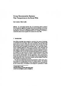
We utilize decision trees to initiate a profile for a new user. In particular we are using the top-down lazy decision tree (LazyDT) described in [4] as the base algorithm. However we are using a different splitting criterion described in Eq. 5 as the splitting criterion. The pairwise comparisons are located at the decision nodes. Each node in the tree is associated with a set of corresponding users. This allows the user to quit the profile initialization process anytime she wants. If the user does not wish to answer more questions, we take the list of users that are associated with the current node and calculate the mean of their factorized vectors. The more questions the user answers, the more specific her vector becomes. But even with answering only a few questions we can still provide the user a profile vector. Figure 1 illustrates the root of the decision tree. Each inner node represents a different pairwise comparison. Based on the response to the first (root) question, the decision tree is used to select the next pairwise comparison to be asked. Note that one possible outcome is ”unknown”, this option is selected when the user does not recognize the items. Every path in the decision tree represents a certain set of comparisons that the user is asked. Assuming that there are k clusters, then the longest possible path contains k·(k−1) inner nodes 2 (comparisons).

Fig. 1.

An illustration of the pairwise decision tree.

Note that if there are s possible outcomes in each pairwise comparison and there are k clusters, then the complete decision tree will have sk∗(k−1)/2 leaves. Even for moderate values of k this becomes impractical. Thus, instead of building the entire decision tree, we take the lazy approach. If the current newcomer has reached a leaf and is willing to answer additional questions, only then do we expand the current node using the suggested splitting criterion. In this way, the tree expands gradually and on-demand. Given a limited memory size, we keep only the most frequent visited nodes. A. Predicting ratings Since each tree node is associated with a set of users, we can create a new user profile vector for each node by taking the mean of the vectors of the corresponding users. When a user decides to terminate the profile initialization, we generate

5

her profile vector pu based on the node she has reached on the tree. Then Eq. 1 can be used to predict ratings. But for that we need to know the user bias. To do this, we first reconstruct the user’s supposed individual ratings ru,i ˜ . We distinguish supposed ratings from original ones by using the tilde notation. Supposed ratings are pairwise responses that are converted to ratings using the right dominant eigenvector mapping procedure presented above. In order to estimate bu , we solve the least squares problem presented in Eq. 2 by replacing ru,i with ru,i ˜ . Note that in this case the parameters pu , qi , bi and µ are fixed. Thus we need to minimize an univariate function with respect to bu over the domain [−5, +5] (when ratings range from 1 to 5). Minimization is performed by the golden section search. VI. E XPERIMENTAL S TUDY In order to evaluate the proposed method for eliciting initial preferences and to examine its effect on recommendations, we conducted an extensive field study on real users. The main goal of this study was to examine the efficiency of the questionnaire-based, pairwise model for eliciting user profiles. The performance of the proposed method was compared to alternative elicitation methods. Since previous researches utilized individual item ratings, it was sufficient to use a simulation over existing datasets in order to evaluate the method being studied. In our case we use pairwise comparisons that could not be obtained directly from publicly available datasets. Thus we took the following approach. We first used the Netflix dataset for creating the initial SVD model. Then we conducted a field study in which we asked more than 400 subjects to respond to a set of 100 pairwise questions and to rate 250 items that were selected from the Netflix item catalog. We compared the profiles that were derived from the pairwise responses with the profiles induced from the simple ratings. In order to present users with as lively a questionnaire as possible, we had to display movie posters. To this end, we used the Internet Movie Database. Our approach was compared to the three top methods for generating initial profiles: GreedyExtend , IGCN and Popularity. In addition we compared our process for selecting the pair of clusters with random selection of the pairs.

the system. However setting k to a moderate value, ensures that it is possible to search the pairwise space with a limited computational effort and thus can be performed online. B. Data collection In order to compare the various methods, 418 users from two countries (Israel and Germany) participated in the study. Two thirds of the participants were undergraduate students. Sixty two percent of the participants were male. Each subject was asked to complete a six-part questionnaire via a Web-based application. The first part contained 50 pairwise questions. These questions cover a small portion of the judgment matrix. Since we partitioned the items in this experiment into 100 clusters, there were exactly 99*100/2=4950 different pairs. The questions were determined by the system (based on a lazy decision tree). Thus in this first part, each user answered a potentially different set of questions. In the second part, an additional 50 pairwise questions, randomly selected, were presented to the user. Note that the clusters were selected randomly. But once they were selected we chose representative items according to the same procedure presented in section IV-D. Parts 3, 4 and 5 contained 50 single-item rating (1 to 5 stars) requests each. The requests corresponded to the top 50 items obtained from each compared method: GreedyExtend , IGCN and Popularity. The last part contained 100 single-item rating questions that were used as a test set for evaluating the efficiency of the elicitation processes. The items in the test set and the items presented in the other parts were mutually exclusive. All users responded to all parts of the questionnaire but in a certain permutation that was determined using a Latin square design in order to reduce the risk of a carryover effect. C. Measuring the Performance We measured the quality of the results by the root-meansquare error (RMSE). We performed the entire procedure for each method for every participant. We computed an average RMSE across all participants equally, rather than biasing the results towards participants with more ratings. In addition to the quality aspect, we also measured how many questions the users have skipped.

A. Values of the experimental parameters

D. Results and Discussion

As in [7] we used the following values for the SVD meta parameters: γ = 0.005, λ4 = 0.02. The parameter γ indicates the learning rate of the gradient descent optimization method used for solving Eq. 2. We also used 200 factors (i.e. f = 200). While accuracy is improved as more factors are used, it has been shown that for NetFlix data, using more than 200 factors would slow running time without significantly improving performance [7] As with the clustering phase, any clustering algorithm can be used. This work employs the popular k-means algorithm [8]. We group the items into k=100 clusters. In a preliminary pilot we also tested two other k-values: k=50 and k=200. The preliminary results indicate that using higher values of k slightly improve the performance. Thus one can use additional clusters and potentially improve the perceptivity of

Figure 2 presents the RM SE performance of five different methods: Popularity; GreedyExtend; IGCN and three pairwise methods. The label PWDT refers to our technique which uses pairwise clustered items whose order of presentation is defined by the proposed lazy decision tree procedure. The PWRandom algorithm refers to usage of pairwise clustered items presented in a random order. The results indicated that all methods improved as more information became available. The plots of Figure 2 show that even with a small number of pairwise comparisons, it was possible to obtain good quality. The proposed method demonstrated a major accuracy improvement when compared to static methods (such as Popularity and GreedyExtend). The improvement is also illustrated when PWDT is compared to a dynamic algorithm (IGCN) although in this case the

6

improvement is less prominent. Additionally, PWDT significantly outperformed PWRandom, indicating that pairwise comparisons should be chosen carefully. Although the idea of clustering the items gives up the fine granularity advantage of item-based pairwise comparison, it still obtains low RMSE.

Fig. 3. Number of users that skipped a question as a function of the progress in the elicitation process.

Fig. 2. Comparison of initial profile generation methods. Accuracy is measured by RMSE. Lower values indicate better performance.

To examine the effects of the total number of questions and of the elicitation method, a two-way analysis of variance (ANOVA) with repeated measures was performed. The dependent variable was the mean RMSE. The results of the ANOVA showed that the main effects of the number of questions F (49, 20433) = 17.3, p < 0.001 and the algorithm F (4, 1668) = 12.66, p < 0.001 were both significant. The post-hoc Duncan test was conducted in order to examine whether the proposed pairwise technique outperformed the four other methods. With α = 0.05, starting from the third question our method was significantly better than randomly selecting the pairwise questions. From the fifth question our technique was significantly better than all single-item algorithms. One can safely conclude that the proposed pairwise questionnaire for preference elicitation is efficient if a user answers a relatively small number of questions. Figure 3 specifies the number of users that skipped a question as a function of the progress in the elicitation process. All methods except PWRandom showed a moderate increase in the number of users that skipped the question. The random method was approximately constant across all iterations. In respect to the skipping rate, the proposed pairwise method was slightly worse than single-item rating methods. This can be partially explained by the fact that in pairwise cases the user might skip the question if she did not know one of the movies. Theoretically if the probability for not knowing a single movie is p, then the probability for not knowing at least one movie in a pair is: p2 = 1 − (1 − p)(1 − p) = p(2 − p) ≥ p. With p = 0.2 (which is the approximate skip rate in our experiment), we expect p2 = 0.36 which is significantly higher than p. Nevertheless, in the current experiment the differences were not so noticeable. This might indicate that users can provide a pairwise feedback even if they are not able to accurately rate each item separately. This happens, for example, when the user has clear opinions about the known item (i.e., she either extremely likes or dislikes the item). VII. C ONCLUSIONS AND F UTURE W ORK We presented a pairwise comparison method for initially generating user profiles. The method uses a decision tree-like

algorithm that adapts the questions to the user. Our empirical study showed an improvement in accuracy when compared to single item rating methods (either static or dynamic). Due to time and space limitations, our proposed model can be calculated in advance only for a small set of clusters. Hence, for large scale systems certain computations must still be done online. We are planning to introduce a caching mechanism that will reduce these computational effort to a minimum. Moreover, we are in the process of extending our algorithm to account for implicit feedback. Finally the proposed method was compared to several methods. However to get a complete picture the method should also be compared to other latent factor pairwise preferences elicitation methods. [1], [9], [12]. R EFERENCES [1] Balakrishnan S., Chopra S.: Two of a Kind or the Ratings Game? Adaptive Pairwise Preferences and Latent Factor Models. ICDM 2010: 725-730 [2] Choi, S.H. and Jeong, Y.S. and Jeong, M.K., A hybrid recommendation method with reduced data for large-scale application, IEEE Transactions on Systems, Man, and Cybernetics, Part C, 40(5):557-566, 2010. [3] Frias-Martinez, E. and Chen, S.Y. and Liu, X., Survey of data mining approaches to user modeling for adaptive hypermedia, IEEE Transactions on Systems, Man, and Cybernetics, Part C, 36(6):734-749, 2006. [4] Friedman, J.H. and Kohavi, R. and Yun, Y. (1996), Lazy decision trees, Proc. of AAAI. pp. 717–724. [5] Golbandi, N. and Koren, Y. and Lempel, R. (2011), Adaptive bootstrapping of recommender systems using decision trees, Proc. 4th ACM inter. conf. on Web search and data mining, pp. 595–604. [6] Golbandi N. and Koren Y. and Lempel R.(2010), On bootstrapping recommender systems., CIKM’10, pp. 1805–1808. [7] Koren Y., Bell R. (2011), Advances in Collaborative Filtering, In Recommender Systems Handbook, Springer, pp. 145-186. [8] Lloyd., S. P. (1982). Least squares quantization in PCM, IEEE Transactions on Information Theory 28 (2): 129137. [9] Liu N. N., Zhao M., and Yang Q., Probabilistic latent preference analysis for collaborative filtering. In CIKM 09, pages 759 766, New York, NY, USA, 2009. ACM. [10] Rashid A.M., Karypis G., Riedl J., Learning preferences of new users in recommender systems: an information theoretic approach, SIGKDD Explorations, 2008, 10(2): 90-100. [11] Rashid A.M., Albert I., Cosley D., Lam S.K., McNee S.M., Konstan J.A., Riedl J. (2002), Getting to know you: learning new user preferences in recommender systems, IUI, pp. 127–134. [12] Rendle S., Freudenthaler C., Gantner Z., and Schmidt-Thieme L., BPR: Bayesian Personalized Ranking from Implicit Feedback. In UAI 09, 2009. [13] Sarwar, B. and Karypis, G. and Konstan, J. and Riedl, J., Incremental singular value decomposition algorithms for highly scalable recommender systems, Proc. of the 5th Inter. Conf. in Computers and Information Technology(2002). [14] Satty T.L., The Analytic Hierarchy Process: Planning, Priority Setting, Resource Allocation, McGraw-Hill (1980).