Innocent Game Semantics via Intersection Type Assignment Systems simply-typed λ-calculus, a game model for it, based on games à la Abramsky-Jagadeesan-.
Innocent Game Semantics via Intersection Type Assignment Systems∗ Pietro Di Gianantonio and Marina Lenisa Dipartimento di Matematica e Informatica, Università di Udine, Italy {pietro.digianantonio,marina.lenisa}@uniud.it
Abstract The aim of this work is to correlate two different approaches to the semantics of programming languages: game semantics and intersection type assignment systems (ITAS). Namely, we present an ITAS that provides the description of the semantic interpretation of a typed lambda calculus in a game model based on innocent strategies. Compared to the traditional ITAS used to describe the semantic interpretation in domain theoretic models, the ITAS presented in this paper has two main differences: the introduction of a notion of labelling on moves, and the omission of several rules, i.e. the subtyping rules and some structural rules. 1998 ACM Subject Classification F.3.2 Semantics of Programming Languages. Denotational semantics Keywords and phrases Game Semantics, Intersection Type Assignment System, Lambda Calculus. Digital Object Identifier 10.4230/LIPIcs.CSL.2013.231
1
Introduction
Game semantics has been proved a powerful and flexible tool to describe the semantics of programming languages. Its main idea is to define the behaviour of a program as a sequence of elementary interactions between the program and the environment. Intersection types have first been used to provide logical descriptions of domain theory models of λ-calculus [7, 8], but they can be applied to general programming languages. The approach can be outlined as follows. The semantics of the λ-calculus can be given in two forms: a term can be interpreted either denotationally by a point in a particular domain, or logically by a set of properties. Stone-duality, as presented in [1], establishes an equivalence between these two alternative descriptions for suitable categories of domains. In the ITAS approach, properties of terms are normally called “types”. The logical semantics consists of the set of rules which allow to derive the properties satisfied by a term. ITAS can be used to provide concrete, finitary approximations of the semantics of a term. The present work continues the line of research of [10], aiming at correlating the game semantics and ITAS. These two approaches to the semantics of programming languages seem, at first sight, quite distant one from the other, establishing a relation can enlighten a different perspective on them. Moreover, compared to game semantics, intersection types have a simpler and more direct presentation, so it is interesting to consider what aspects of game semantics can be described through them. In [10], the authors have considered a
∗
Work partially supported by the Italian MIUR PRIN Project CINA 2010LHT4KM, and by the ICT COST Action BETTY IC1201.
© Pietro Di Gianantonio and Marina Lenisa; licensed under Creative Commons License CC-BY Computer Science Logic 2013 (CSL’13). Editor: Simona Ronchi Della Rocca; pp. 231–247 Leibniz International Proceedings in Informatics Schloss Dagstuhl – Leibniz-Zentrum für Informatik, Dagstuhl Publishing, Germany
232
Innocent Game Semantics via Intersection Type Assignment Systems
simply-typed λ-calculus, a game model for it, based on games à la Abramsky-JagadeesanMalacaria [2] (AJM games), and a corresponding ITAS. It has been shown that such ITAS gives a precise description of the interpretation of λ-terms in the AJM-game model. In particular, a type t for a term M describes a set of moves that the Proponent and the Opponent may exchange in some phases of the interaction of the term M with the environment, and the set of types assigned to a term gives a complete description of the history-free strategy of the term, seen as a partial function on moves. However, some aspects of game semantics are not captured by the ITAS description of AJM-games, for example in AJM-games the same strategies have several possible descriptions, differing by the use of indexes on moves. In order to capture the equivalence relation between strategies, a notion of equivariance between plays has been introduced. However, in the ITAS description, it is not clear how to capture this equivalence relation in a natural and simple way. In the present work, the aim is to extend results presented in [10], by enlarging the aspects of game semantics that can be described through ITAS, and by considering alternative paradigms of game semantics. In particular, we obtain an ITAS description of innocent games, i.e. games based on innocent strategies. In this way, we show that the ITAS approach can be used for different paradigms of game semantics. Moreover, for innocent games, each strategy has a single representation, therefore a drawback of the ITAS description of AJM-games, namely the missing equivalence relation between alternative representations of the same strategy, is avoided. In more detail, we show that, by introducing in the ITAS a limited set of structural rules, it is possible to describe the interpretation of λ-terms in the framework of innocent games. The structural rules considered state that the ∧ operator satisfies the associative and commutative properties, but not the idempotency. So, from an ITAS perspective, the difference between the two main paradigms of game semantics is reflected by the presence/absence of some structural rules. Technically, intersection types for innocent games carry more structure, since they represent sets of moves which are partitioned via a suitable labelling, and are (implicitly) endowed with justification pointers. Non-idempotent intersection types have been also considered in [15, 16, 9]. In particular, in [15, 16], it has be shown that in non-idempotent ITAS, any term t has a principal type τ that gives a complete description of the normal form of t. In this paper, we chose, for the sake of simplicity, as target language unary PCF, and we provide an innocent game model for it. The ITAS presentation of this model exploit an alternative description of innocent strategies via partitioned positions, which we introduce in this paper. Given a play on a game A, by forgetting the linear order along with moves are played, one obtains a set of moves together with justification pointers. We call this kind of structure position. A partitioned position is a play where only part of the information concerning the order in which the moves have been laid down has been omitted. In the ITAS that we present, types correspond to partitioned positions. The induced type semantics turns out to provide the same theory of the game semantics. When simple positions without partitions are considered, the corresponding types and ITAS result simplified, however the theory induced by the game semantics is strictly included in that induced by the type semantics. The idea to remove, partially or completely, the order information on games has been considered several times in the literature [3, 12, 14, 4, 6]. In [3], timeless games are used to build a model for classical linear logic. In timeless games the order on plays is completely forgotten as in the presentation of innocent strategies via simple positions. In [4], it has been shown that the operation of forgetting the time order can be described by a suitable functor. In [14], it has been shown that, for the particular class of asynchronous games, a
P. Di Gianantonio and M. Lenisa
233
strategy can be completely characterized by the set of its positions. In [12, 6], a faithful functor from the category of games to a category of relations is presented, that forgets part of the time order along with moves are played. Synopsis. In Section 2, we recall basic definitions and constructions on arenas and innocent strategies. In particular, we provide a characterisation of innocent strategies via partitioned positions. In Section 3, we present a game model of unary PCF. In Section 4, we introduce and study an ITAS giving a finitary description of the model of Section 3. In Section 5, we establish the connection between the ITAS and the game model of unary PCF. Finally, in Section 6, we discuss further developments. Acknowledgements. The authors thank the anonymous referees for their comments, which allowed to improve the presentation of the paper.
2
The Category of Arenas and Innocent Strategies
In this section, we recall basic notions and constructions on arenas and innocent strategies in the style of [11]. Notice that we define justification sequences as containing exactly one initial move. The following are the usual definitions of arena and strategy: I Definition 1 (Arena). An arena has two participants: the Proponent and the Opponent. An arena is specified by a triple A = (MA , λA , `A ), where MA is the set of moves. λA : MA → {OQ, OA, P Q, P A} is the labelling function: it tells us if a move is taken by the Opponent or by the Proponent, and if it is a question or an answer. We denote by − the function which exchanges Proponent and Opponent. `A is a relation between MA + {?} and MA , called enabling, which satisfies ? `A a =⇒ (b `A a ⇔ b = ?) ∧ λA (a) = OQ, and a `A b ∧ a 6= ? =⇒ a is a question, i.e. π2 ◦ λA (a) = Q, and π1 ◦ λA (a) 6= π1 ◦ λA (b). The enabling relation tells us either that a move a is initial and needs no justification (? `A a), or that it can be justified by another move b, if b has been played (b `A a). I Definition 2. A justified sequence s of moves in an arena A is a sequence of moves together with justification pointers such that: the first move is the only initial move, and for each other move a in s there is a pointer to an earlier move b of s such that b `A a. We say that the move b justifies the move a, and we extend this terminology to say that a move b hereditary justifies a if the chain of pointers back from a passes through b. Given a justified sequence s, the view of s, view(s), also called P-view, is defined as follows: view(�) = �, where � denotes the empty sequence, view(s · a) = a, if s = � or a is an initial move, view(s · a · t · b) = view(s) · a · b, if the move b is justified by a. If s is a justified sequence containing a move a, we say that a is visible at s if a appears in view(s). A non-empty justified sequence s is a play iff O moves first: s = as0 and π1 ◦ λ(a) = O s is alternating: if s = s1 abs2 then π1 ◦ λ(a) 6= π1 ◦ λ(b) the visibility condition holds: if s = s1 as2 , and a is not initial, then the justifier of a is visible at s1
CSL’13
234
Innocent Game Semantics via Intersection Type Assignment Systems
the well-bracketing condition holds: if s = s1 as2 , and a is an answer, then it must be justified by the most recent unanswered question. The set of plays of an arena A is denoted by PA . Notice that the above definition is slightly different from the standard one: plays are not empty, and the initial move is unique. This presentation will provide a better correspondence with the intersection type assignment system. I Definition 3 (Strategy). A strategy for the Proponent on an arena A is a set σ ⊆ PAeven of plays of even length such that: sab ∈ σ =⇒ s ∈ σ and sab, sac ∈ σ =⇒ b = c . A strategy σ on an arena A is innocent if for all sab, t ∈ σ, if ta ∈ PA and view(sa) = view(ta), then also tab ∈ σ, with b justified by the same element of view(ta) = view(sa) as in sab. A strategy can be seen as a set of rules which tells the Proponent which move to take after the last move by the Opponent. Innocent strategies are strategies which depend only on the view.
Constructions on Arenas I Definition 4 (Product). Given arenas A and B, the product A × B is the arena defined as follows: MA×B = MA + MB λA×B = [λA , λB ] ? `A×B m ⇐⇒ ? `A m ∨ ? `B m and m `A×B n ⇐⇒ m `A n ∨ m `B n. Here + denotes disjoint union of sets, that is A + B = {(l, a) | a ∈ A} ∪ {(r, b) | b ∈ B}, and [−, −] is the usual (unique) decomposition of a function defined on disjoint unions. The unit for × is I = (∅, ∅, ∅). I Definition 5 (Implication). Given games A and B, the compound game A → B is defined as follows: MA→B = MA + MB λA→B = [λA , λB ] ? `A→B m ⇐⇒ ? `B m and m `A→B n ⇐⇒ m `A n ∨ m `B n ∨ (? `B m ∧ ? `A n).
The Game Category G Objects: arenas. Morphisms: a morphism between arenas A and B is an innocent strategy σ on A → B. Composition: given innocent strategies σ : A → B and τ : B → C, τ ◦ σ : A → C is defined by: τ ◦ σ = {s � (A, C) | s ∈ σ||τ }even , where σ||τ = {s ∈ (MA + MB + MC )∗ | s � (A, B) ⊆ σ & s � (B, C) ∈ τ }, with s � (A, B) denoting the subsequence of s consisting of moves in A and B. Identity: id A : A → A, id A = {s ∈ PAeven | ∀t even-length prefix of s. t�1 = t�2} , where t�1 (t�2 ) denotes the restriction of s to the first (second) A component. The arena constructions of product and implication can be made functorial, in such a way that I Proposition 6. The category G is cartesian closed with × as cartesian product and → as exponential. The arena I is the terminal object of the category G.
P. Di Gianantonio and M. Lenisa
2.1
235
An Alternative Description of Innocent Strategies
The type assignment system we present describes the strategies associated to λ-terms in an indirect way. To establish the connection between ITAS and games semantics interpretation it is necessary to introduce an alternative description of strategies. Instead of describing an innocent strategy by a set of plays, we describe it by a set of partitioned positions. Given a play on a game A, by forgetting the linear order along with moves are played, one obtains a set of moves together with justification pointers for all moves but one (the initial move). We call this kind of structure position. For a particular class of games, i.e. the asynchronous games, Melliès [14] shows that a strategy is completely characterised by the set of its positions. This result is not anymore true for generic innocent games. We therefore introduce the new concept of partitioned position. A partitioned position is a play where only part of the information concerning the order in which the moves have been laid down has been omitted. The innocence condition on strategies assures that using the reduced information allows to reconstruct the original full description of the strategy. I Definition 7 (Partitioned Position). Let A be an arena. We define a position on the arena A as an unordered tree, whose nodes are (instances) of moves on A and such that 1. the root is an initial move, 2. for any node n, all children of n are moves enabled by n. We denote by (m, {p1 , . . . , pn }) the position with root m and subtrees p1 , . . . , pn . A partitioned position is a pair (p, Ep ), formed by a position p and a partition Ep on the nodes of p. On partitioned positions we consider the partial order j given by (p, Ep ) j (p, Ep0 ) if Ep is a partition finer than Ep0 , i.e. each equivalence class of Ep is contained in an equivalence class of Ep0 . Since a partition Ep can be also seen as an equivalence relation, for convenience, in some definitions, we will treat Ep as an equivalence relation. I Definition 8 (Position from Play). Given a play s on the arena A, we denote by [s]∗ the partitioned position (p, Ep ), where the position p is formed by the moves in s together with their justification pointers (a move n is a child of a move m in p if and only if n is justified by m in s); two distinct moves m, n lie in the same set of the partition Ep if and only if m is an Opponent move, and n is the Proponent move immediately following m in the play s. Given a strategy σ on the arena A, we denote with [σ]∗ the set of partitioned positions {(p, Ep ) | ∃s ∈ σ . [s]∗ j (p, Ep )}. The function [ ]∗ on plays is not injective, that is there can be two distinct plays s and t generating the same partitioned position. This is due to the fact that from the partitioned position [s]∗ it is not possible to completely recover the linear order of moves in a play s. However, the function [ ]∗ is injective on P-views, in fact, given a P-view s and any move m in [s]∗ , it is possible to define the predecessor of m in s: if m is a Proponent move then its predecessor is the Opponent move laying in the same partition, while if m is an Opponent move, by P-view definition, the predecessor of m is its parent in the tree. Since an innocent strategy is uniquely determined by the set of P-views that it contains ([11], Section 5.2), it follows that the function [ ]∗ is injective on innocent strategies. Moreover, from the set [σ]∗ , it is possible to reconstruct the innocent strategy σ. In fact, given a partitioned position (p, E), it is decidable to check if (p, E) is the image of a P-view s along [ ]∗ , and in this case to reconstruct the P-view s. Therefore, from [σ]∗ , it is possible to define the set of P-views
CSL’13
236
Innocent Game Semantics via Intersection Type Assignment Systems
of σ, and using the construction presented in [11] Section 5.2, from the set of P-views one can define the set of plays of σ. On the sets of partitioned positions it is possible to define an operation of composition in the following way. A partitioned position (q, Eq ) on the arena A → B can be decomposed in a partitioned position on B, denoted by (q, Eq ) � B, and in a multiset of partitioned positions in A, denoted by (q, Eq )�A. In more detail, if q = (m, {p1 , . . . , pm , q1 , . . . , qn }) with p1 , . . . , pm having moves in B and q1 , . . . , qn having moves in A, (p, Ep ) � B is the position (m, {p1 , . . . , pm }) with the inherited partition. The multiset (p, Ep )�A is composed of the multiset of positions {q1 , . . . , qn } with the inherited partitions. I Definition 9 (Composition). A finite multiset of partitioned positions {(q1 , Eq1 ), . . . , (qn , Eqn )} in A → B and a partitioned position (p, Ep ) in B → C compose if (p, Ep )�B = {(q1 , Eq1 )�B, . . . , (qn , Eqn )�B}. In this case, the composition {(q1 , Eq1 ) . . . (qn , Eqn )} ◦ (p, Ep ) is defined as the position: [ (m, {p1 , . . . , pm } ∪ {qi,1 , . . . , qi,ni } ) , i∈{1,...,n}
under the hypothesis that (p, Ep ) � C = ((m, {p1 , . . . , pm }), Ep0 ) and (qi , Eqi ) � A = {(qi,1 , Eqi,1 ), . . . , (qi,ni , Eqi,ni )}. On the above position we define a partition E as follows: two nodes m, n are related by E iff one of the following conditions holds: – the nodes m, n are related either by Ep or by Eqi ; – there exist an index i and a node m0 in the arena B such that (m, m0 ) ∈ Ep and (n, m0 ) ∈ Eqi ; – there exist indexes i, j and nodes m0 , n0 in the arena B such that (m, m0 ) ∈ Eqi , (n, n0 ) ∈ Eqj , and (m0 , n0 ) ∈ Ep . Given two sets of partitioned positions S in B → C and T in A → B, the composition S ◦ T is defined by {{(q1 , Eq1 ), . . . , (qn , Eqn )}◦(p, Ep ) | {(q1 , Eq1 ), . . . , (qn , Eqn )} ⊆ S, (p, Ep ) ∈ T compose}. With the above definition of composition, arenas and sets of partitioned positions form the objects and the arrows of a category. It is possible to refine the notion of partitioned position by defining the notion of well-formed partitioned position characterizing those positions that are the image, along [ ]∗ , of a play. Then one can further define a subcategory having as arrows sets of well-formed partitioned positions. In this subcategory the function [ ]∗ defines the arrow part of a faithful functor from the category of innocent strategies to the one of sets of partitioned positions. However, in the present work we omit this lengthy definition of the category, and we just prove the main property that will be used in the rest of the paper: the function [ ]∗ on strategies preserves composition. The proof of the proposition below appears in the Appendix. I Proposition 10. For any pair of innocent strategies σ : A → B and τ : B → C, we have that [τ ◦ σ]∗ = [τ ]∗ ◦ [σ]∗ .
2.2
Timeless Games
It is worthwhile to notice that the construction presented above can be repeated using the simpler notion of position, instead of partitioned position. Along this line, one can define a notion of composition between sets of positions, and a function [ ]• that associates to
P. Di Gianantonio and M. Lenisa
237
a strategy the set of positions of its plays. As corollary of Proposition 10, one can show that also the function [ ]• preserves composition. Although presented in different form, the function [ ]• appears in [4]. In this work, positions are described as relations, and it has been shown that [ ]• constitutes the arrow part of a functor from the category of arenas and innocent strategies to a suitable category of sets and relations. It turns out that positions are not sufficient to describe innocent strategies, in that it can be the case that two different innocent strategies are mapped to the same set of positions, see at the end of Section 3 below for an example.
3
A Game Model of Unary PCF
In this section, we define a game model of unary PCF. We chose to consider unary PCF, since it is a simple language, with a minimal set of constants, and it allows for a concise presentation of our ITAS. However, the ideas presented in this paper can be immediately extended to more elaborated functional languages with call-by-name reduction. Models of unary PCF have been extensively studied in the literature, especially extensional ones, see e.g. [13, 5]. Here we are interested in the intensional game model arising from the Sierpinski arena, which induces the theory of normal forms. In Section 4, we will provide a description of this model via a type assignment system. We recall that unary PCF is a typed λ-calculus with two ground constants, ⊥, >, and a sequential composition constant &1 , which takes two arguments of ground type: if its first argument is >, then & returns its second argument, otherwise, if its first argument is ⊥, then & returns ⊥.
Unary PCF I Definition 11. The class SimType of simple types over a ground type o is defined by: (SimType 3) A ::= o | A → A . Raw Terms are defined as follows: Λ 3 M ::= ⊥ | > | & | x | λx : A.M | M M , where ⊥, >, & are constants, and x ∈ Var. We denote by Λ0 the set of closed λ-terms. Well-typed terms. We introduce a proof system for deriving typing judgements of the form ∆ ` M : A, where ∆ is a type environment, i.e. a finite set x1 : A1 , . . . , xk : Ak . The rules of the proof system are the following: ∆ `⊥: o
∆`>:o
∆, x : A ` M : B ∆ ` λx : A.M : A → B
∆`&:o→o→o
∆, x : A ` x : A
∆`M :A→B ∆`N :A ∆ ` MN : B
Conversion rules. The conversion relation between well-typed terms is the least relation generated by the following rules together with the rules for congruence closure (which we omit): ∆ ` (λx : A.M )N = M [N/x] ∆ ` &⊥M = ⊥ ∆ ` &>M = M ∆ ` &M > = M 1
In the literature, this constant is usually denoted by ∧; here we prefer to denote it by &, since the symbol ∧ is used in the intersection type assignment system.
CSL’13
238
Innocent Game Semantics via Intersection Type Assignment Systems
Notice that the conversion rules for & include reductions where the first or the second argument is >, but only the reduction where the first argument is ⊥. The reduction in the case the second argument is ⊥ is omitted, in order to keep the correspondence between normal forms and strategies (see Theorem 15 below).
Game Model In the cartesian closed category G, simple types are interpreted by the hierarchy of arenas over the following Sierpinski arena: I Definition 12 (Sierpinski Arena). The arena O is defined as follows: MO = {q, a} λO (q) = OQ λO (a) = P A ? `O q and q `O a In the game model, terms in contexts are interpreted as innocent strategies in the usual way, using standard categorical combinators, i.e. x1 : A1 , . . . , xk : Ak ` M : A is interpreted as a strategy on the arena [[A1 ]]G × . . . × [[Ak ]]G → [[A]]G . Before giving the formal interpretation of terms, we first need to define the interpretation of constants. Interpretation of the basic constants. The interpretation of the constants ⊥, > is given by the two strategies on the Sierpinski arena: [[⊥]]G is the empty strategy, while [[>]]G = {qa}. The interpretation of the constant & is the strategy [[&]]G on the arena O → O → O, defined by the set of plays generated by the even-prefix closure of the play (r, (r, q))(l, q)(l, a)(r, (l, q))(r, (l, a))(r, (r, a)) (where justification pointers are omitted).
[[&]]G
: O
−→
O
−→
O
e c a =/ qL ~ i g l � � n � q � �J
� a � � � ! q �J " a $
a Given an arena A, we denote by !A the unique empty strategy from the arena A to the terminal arena I. With the obvious isomorphism, a strategy on the arena A can also be seen as a strategy on the arena I → A. The complete definition of the type and term interpretation in the model is the following: I Definition 13 (Type and Term Interpretation). Type interpretation: [[o]]G = O [[A → B]]G = [[A]]G → [[B]]G . Term interpretation: [[x1 : A1 , . . . , xk : Ak ` c : A]]G = [[c]]G ◦![[A ]]G ×...×[[A ]]G if c is a constant. 1 k [[x1 : A1 , . . . , xk : Ak ` xi : Ai ]]G = πi : [[A1 ]]G × . . . × [[Ak ]]G → [[Ai ]]G [[∆ ` λx : A.M : A → B]]G = Λ([[∆, x : A ` M : B]]G ) [[∆ ` M N : B]]G = ev ◦ h[[∆ ` M : A → B]]G , [[∆ ` N : A]]G i where πi denotes the i-th projection, ev denotes the natural transformation, and Λ denotes the functor characterizing G as cartesian closed category. Using standard methods, one can prove that the theory induced by the game model is the theory of βη-normal forms. The notions of β-normal forms and βη-normal forms on unary PCF are the following:
P. Di Gianantonio and M. Lenisa
239
I Definition 14 (β-normal forms, βη-normal forms). (i) A typed term ∆ ` M : A is in β-normal form if M ≡ λx1 : A1 . . . xn : An . ⊥ or M ≡ λx1 : A1 . . . xn : An .> or M ≡ λx1 : A1 . . . xn : An .&M M 0 , where M, M 0 are in β-normal form, M 6= ⊥, >, and M 0 6= >, or M ≡ λx1 : A1 . . . xn : An .xi M1 . . . Mqi , where M1 , . . . , Mqi are in β-normal form. (ii) A typed term ∆ ` M : A is in βη-normal form if it is in β-normal form and each occurrence of a variable x of type B1 → . . . → Bk → o in M appears applied to k arguments of types B1 , . . . , Bk , respectively. We omit the proof of the following theorem, which is standard: I Theorem 15. The theory Th G induced by the game model [[ ]]G is the βη-theory. In view of the results in [13], the extensional quotient of the above game model is universal for the observational equivalence on unary PCF (see [13] for more details). I Example 16. We conclude this section by providing an example of two different innocent strategies with the same set of positions. Namely, let us consider the terms P ≡ λx : o → o → o.λy : o.x(x ⊥ (& y ⊥))(x ⊥⊥) and Q ≡ λx : o → o → o.λy : o.x(x ⊥⊥)(x(& y ⊥) ⊥). Then, the strategies σP and σQ interpreting P and Q are different for only two plays: σP : (O → O → O) → O → O σQ : (O → O → O) → O → O b _/ j g d q n 6E q m � t b _/ q p
w jg d m { p � q ~ � � � o e0q } � q � q
b _/ j g d q n 6E q m � p t o e0q
w } { � q ~ � � b _/ q � jg d � pm q � q
The first play is contained in σP but not in σQ , while the second one is contained in σQ but not in σP . However, the two plays above induce the same position, so as all plays extending them, and hence the strategies interpreting P and Q have the same sets of positions.
4
The Type Assignment System
In this section, we introduce and study a type assignment system, which gives a finitary description of the game model of Section 3. The types involved are essentially the standard intersection types, where some structural rules are missing. Our approach to intersection types is “typed”, i.e. intersection types are built inductively over arenas. The usual untyped intersection semantics (for the untyped λ-calculus) can be recovered as a special case of the typed case. Intuitively, a type on an arena A represents a partitioned position induced by a play on A. Types on the Sierpinski arena are just sets of moves contained in the possible plays on this arena. As a further ingredient, moves in types are indexed on natural numbers. Indexes are used to describe partitions: two moves lie in the same partition if and only if they have the same index. A type (t1 ∧ . . . ∧ tn ) → t on the arena A → B represents a partitioned position composed by a partitioned position on B, described by t, and several partitioned positions
CSL’13
240
Innocent Game Semantics via Intersection Type Assignment Systems
on A, described by the types t1 , . . . , tn . In this approach, the intersection type constructor (∧) is used to build types on exponential arenas, possibly having multiple instances of the same move. Consequently, the ∧ constructor is not idempotent. The formal correspondence between the type semantics and the game semantics is established in Section 5. We define a syntax for types that is more complex than the standard one for intersection types. The extra conditions we put on types reflect the alternating and well-bracketing conditions on plays. Namely, for each arena A, we define the set of corresponding intersection A types, which divides into P-types (tA P ) and O-types (tO ), i.e. types representing partitioned positions where the Proponent is next to move and types representing partitioned positions where the Opponent is next to move, respectively. Moreover, O-types are divided into “resolved types” (tA Or ), which are intended to represent plays with no pending questions, and “pending types” (tA Op ), which represent plays with pending questions. Notice that all P-types are pending types in this sense. I Definition 17 (Types). We define two families of types, i.e. Proponent types (P-types), A {Type A P }A , and Opponent types (O-types), {Type O }A , these latter are divided into Opponent resolved types and Opponent pending types, by induction on the structure of the arena A via the following abstract syntax: Types on Sierpinski arena: O (Type O P 3) tP ::= {qi }
O (Type O O 3) tOr ::= {qi , aj }
i, j ∈ N
Types on arrow arenas: B !A B (Type A→B 3) tA→B ::= t!A P P Or → tP | tOp → tP B (Type A→B 3) tA→B ::= t!A O Or Or → tOr B !A B !A B (Type A→B 3) tA→B ::= t!A O Op Or → tOp | tOp → tOp | tP → tP
where
!A A A !A (MType !A | t!A O 3) tOr ::= tOr | ∅ Or ∧ tOr !A A !A !A !A !A (MType !A O 3) tOp ::= tOp | tOp ∧ tOp | tOp ∧ tOr !A A !A !A !A !A (MType !A P 3) tP ::= tP | tOr ∧ tP | tOp ∧ tP
!A ∅A denotes the empty type on A, and MType !A P (MType O ) denotes the set of Proponent multiple types (Opponent multiple types). A !A !A Moreover, we define Type A = Type A = MType !A P ∪ Type O , MType P ∪ MType O , Type = S S A !A A A !A !A to denote A Type , and MType = !A MType . We use the symbols t , u , and t , u A !A !A A A !A !A types and multiple types respectively, and the symbols tA , u (t , u ) and t , u P P P P O O (tO , uO ) to denote P (multiple) types and O (multiple) types, respectively. Finally, we endow the types with the equivalence relation induced by: !A !A !A (commutativity) ∅A ∧ t!A = t!A (identity) t!A 1 ∧ t2 = t2 ∧ t1 !A !A !A !A !A !A (t1 ∧ t2 ) ∧ t3 = t1 ∧ (t2 ∧ t3 ) (associativity) .
In the definition of types, justification pointers are not explicitly represented, but they can be recovered from the structure of types.
P. Di Gianantonio and M. Lenisa
241
I Example 18. The partitioned positions describing the copycat strategy on the arena O → O are induced by the types {q0 } → {q0 } and {q0 , a1 } → {q0 , a1 }. Notice that, since the type {q0 , a1 } → {q0 , a1 } contains as subexpression the type {q0 , a1 }, the grammar for types needs to generate also types where all indexes are distinct. To make a more complex example, the two plays that differentiate the strategies σP and σQ in Example 16 are described by the types: (({q1 } → ∅O → {q0 }) ∧ (∅O → {q2 } → {q1 })) → {q2 } → {q0 } (({q2 } → ∅O → {q1 }) ∧ (∅O → {q1 } → {q0 })) → {q2 } → {q0 } Notice that types on the arena O → O containing a single move are P-types in the form ∅ → {qi }, while types containing two moves are either Opponent resolved types in the form ∅ → {qi , aj } or Opponent pending types in the form {qj } → {qi }. !A Since the grammar does not contain the production t!A P ∧tP , the type ({q0 }∧{q1 }) → {q0 } does not belong to the grammar; this type describes a play not respecting the alternating condition. B Since the grammar does not contain the production t!A Op → tOr , the type ({q1 } → {q0 }) → {q0 , a1 }) does not belong to the grammar; this type describes a play not respecting the bracketing condition. I Definition 19 (Environments). Environments Γ are finite sets {x1 : t1!A1 , . . . , xk : tk!Ak } with the variables x1 , . . . , xk all distinct. For simplicity, we omit braces in writing the environments. The symbol Γ∅ stands for an environment in the form x1 : ∅A1 , . . . , xk : ∅Ak . Given two environments Γ, Γ0 in the form Γ = x1 : t1!A1 , . . . , xk : tk!Ak and Γ0 = x1 : 0 0 0 0 !Ak k t1!A1 , . . . , xk : tk!Ak , we define Γ∧Γ0 as the environment x1 : t1!A1 ∧t1!A1 , . . . , xk : t!A k ∧tk We introduce a typing system for deriving judgements of the shape x1 : t1!A1 , . . . , xk : ` M : tA , whose intended meaning is to represent a partitioned position in the strategy interpreting the term M in the game model of Section 3.
k t!A k
I Definition 20 (Typing System). The typing rules for deriving judgements x1 : t1!A1 , . . . , xk : k t!A ` M : tA are the following: k i∈N Γ∅ ` > : {qi , ai } i∈N Γ∅ ` & : {qi } → ∅O → {qi } i, j ∈ N Γ∅ ` & : {qi , aj } → {qj } → {qi } i, j, k ∈ N Γ∅ ` & : {qi , aj } → {qj , ak } → {qi , ak } tA ∈ Type A Γ∅ , x : tA ` x : tA
(>)
(&1 ) (&2 ) (&3 )
(var)
CSL’13
242
Innocent Game Semantics via Intersection Type Assignment Systems
Γ, x : u!A ` M : tB Γ ` λx : A.M : u!A → tB A B Γ ` M : uA Γ1 ` N : uA ... 1 ∧ . . . ∧ un → t 1 B Γ ∧ Γ1 ∧ . . . ∧ Γn ` M N : t
(abs)
Γn ` N : uA n
Γ ` M : ∅A → tB Γ ` N : A Γ ` M N : tB
(app)
(app’)
where Γ denotes the simple type environment induced by Γ. Notice that, in the judgements derivable in the typing system above there is a clear separation between types appearing in the left part (i.e. in the environment) and types appearing in the right part: namely, the types in the left part are multiple types, while in the right part only (arrow) types appear. The extra rule for application (app0 ) is necessary because the expression ∅A only belongs to the grammar of multiple types but not to the grammar of types. I Example 21. By the axioms: x : ∅O→O→O , y : ∅O ` & : {q2 } → ∅O → {q2 } , x : ∅O→O→O , y : {q2 } ` y : {q2 } , x : ∅O → {q2 } → {q1 }, y : ∅O ` x : ∅O → {q2 } → {q1 } , x : {q1 } → ∅O → {q0 }, y : ∅O ` x : {q1 } → ∅O → {q0 } , using the rules (app) and (app0 ), we get x : ∅, y : {q2 } ` &y⊥ : {q2 } . Again by the rules (app0 ) and (app), x : ∅O → {q2 } → {q1 }, y : {q2 } ` x⊥(&y⊥) : {q1 } . By the rules (app) and (app0 ), x : ({q1 } → ∅O → {q0 } ∧ ∅O → {q2 } → {q1 }), y : {q2 } ` x(x⊥(&y⊥))(x⊥⊥) : {q0 } , and by a double application of the rule (abs), ` λx : o → o → o.λy : o.x(x ⊥ (& y ⊥))(x ⊥⊥) : (({q1 } → ∅O → {q0 }) ∧ (∅O → {q2 } → {q1 })) → {q2 } → {q0 } . Notice that the following rule is admissible: Γ ` M : tA φ : N → N Γφ ` M : tA φ
(sub)
where φ is a generic a function on natural numbers and tA φ denotes the type tA where all indexes on moves are substituted according to the function φ. The rule (sub) can be usefully employed on the premises of the rule (app), in order to derive premises sharing identical indexes on the corresponding types. Notice that, to obtain this result, it can be necessary to identify different indexes, and so the function φ, used as parameter in sub, needs to be a general function and not simply a permutation. The fact that the types in any derivable judgement are well-formed intersection types follows from Lemma 22 below. This lemma can be easily proved by induction on derivations. !Ak 1 I Lemma 22. If x1 : t!A ` M : tA is derivable, then: 1 , . . . , xk : tk !A1 A if t is a resolved O-type, then all t1 , . . . , tk!Ak are resolved O-types; !Ak 1 if tA is a pending O-type, then all t!A are O-types; 1 , . . . , tk if tA is a P-type, then at most one of the types in t1!A1 , . . . , tk!Ak is a P-type.
As a consequence, we have:
P. Di Gianantonio and M. Lenisa
243
!Ak 1 2 1 I Proposition 23. If x1 : t!A ` M : tA is derivable, then (t!A → (t!A → 1 2 1 , . . . , xk : tk !Ak (A1 →(A2 →...(Ak →A))) A . . . (tk → t ))) ∈ Type .
The type assignment system immediately induces a semantics of λ-calculus based on types, whereby any term in context is interpreted by a set of tuples of types as follows: I Definition 24 (Type Semantics). Let [[ ]]T be the interpretation function defined by: !Ak A !Ak !A1 1 [[x1 : A1 , . . . , xk : Ak ` M : A]]T = {(t!A ` M : tA }. 1 , . . . , tk , t ) | x1 : t1 , . . . , xk : tk
5
From Types to Games
In this section, we show that the type semantics coincides with the game semantics. This result follows from the fact that the types appearing in judgements derivable in the intersection type system correspond to partitioned positions in the strategy interpreting the term. In order to formally state this correspondence, it is useful to introduce the notion of indexed position, which is a position where moves are indexed. Clearly, any indexed position determines a partitioned position, where two moves belong to the same partition if and only if they have the same index; we denote by U : IP → P P the natural map from indexed to partitioned positions. Vice versa, any partitioned position determines a class of indexed positions, differing by an injective renaming of indexes. Notice that it would have been possible to use only the notion of indexed position, but we have preferred to introduce also partitioned positions, which provide canonical representatives for strategies. One can easily define a natural map E A : Type A → IP A , for any set of types Type A : I Definition 25. For any set of intersection types Type A , we define E A : Type A → IP A , by induction on the arena A: E O ({qi }) = (qi , ∅) E O ({qi , aj }) = (qi , {(aj , ∅)}). A A E A→B (t!A → tB ) = (m0 , {p01 , . . . , p0k , E A (tA 1 ), . . . , E (tn )}), where A t!A = tA 1 ∧ . . . ∧ tn , B B 0 E (t ) = (m , {p01 , . . . , p0k }), E A (tA i ) denotes the position where the polarity of moves has been reversed, A A the move names in (m0 , {p01 , . . . , p0k , E A (tA 1 ), . . . , E (tn )}) are taken up to the obvious injection in MA + MB . The maps E A can be extended to k + 1-tuple of types (t1!A1 , . . . , tk!Ak , tA ) as follows: I Definition 26. For all MType !A1 , . . . , MType !Ak , Type A , for any k ≥ 0, we define a map E A1 ×...×Ak →A : MType !A1 × . . . × MType !Ak × Type A → IP A1 ×...×Ak →A by induction on the arenas A1 , . . . , Ak , A as follows: for k = 0, E A (tA ) is defined as in Definition 25; !Ak A 1 for k > 0, E A1 ×...×Ak →A (t!A 1 , . . . , tk , t ) = 1 A1 (tA1 ), . . . , E Ak (tAk ), . . . , E Ak (tAk )}) , (m0 , {p01 , . . . , p0h , E A1 (tA 11 ), . . . , E 1n1 k1 knk
where Ai i i t!A = tA i i1 ∧ . . . ∧ tini , for all i, A A 0 0 E (t ) = (m , {p1 , . . . , p0h }), i E Ai (tA ij ), for all i, j, denotes the position where the polarity of moves has been reversed,
CSL’13
244
Innocent Game Semantics via Intersection Type Assignment Systems
1 A1 (tA1 ), . . . , E Ak (tAk ), . . . , E Ak (tAk )}) move names in (m0 , {p01 , . . . , p0h , E A1 (tA 11 ), . . . , E 1n1 k1 knk are taken up to the obvious injection in MA1 + . . . + MAk + MA .
The maps E A and U determine a correspondence between the type semantics and the game semantics, namely: I Definition 27. We define F([[x1 : A1 , . . . , xk : Ak ` M : A]]T ) = !Ak !Ak A !A1 1 ` M : tA } . {U ◦ E A1 ×...×Ak →A (t!A 1 , . . . , t k , t ) | x1 : t 1 , . . . , x k : t k Then, we have the following theorem (whose proof appears in the Appendix): I Theorem 28. (i) For any well-typed term ∆ ` M : A, F([[∆ ` M : A]]T ) = [[[∆ ` M : A]]G ]∗ . (ii) The type semantics and the game semantics induce the same theory.
5.1
ITAS without Indexes
A simplified model for unary PCF can be obtained by using an alternative version of ITAS where types are without indexes. In this alternative version the type semantics of a term M defines the set of positions (and not of partitioned positions) in the strategy [[M ]]G . It turns out that the simplified model does not provide the theory of the game model. The terms P and Q considered in the Example 16 are interpreted in the game model by two different strategies, σP , σQ , containing the same set of positions. More precisely, the theory of the simplified model is intermediate between the theory of the game model and its extensional collapse. Intersection types without idempotency and without indexes have been considered also in [15, 16]. In these works, it has been shown that two terms having the same set of types have also the same normal form. This result is in contrast with what happen in the above sketched ITAS without indexes, where terms P and Q have different normal forms but the same set of types. This difference can be explained by the fact that in our setting the set of types without indexes contains too few elements; in particular on the Sierpinski arena just three types are definable. In contrast, in [15], the untyped lambda calculus and types built over a countable set of type variables are considered. A posteriori, one can argue that, in order to precisely characterize the normal forms of terms, it is necessary to have a sufficiently rich set of types, and the introduction of indexes on types can be seen not only as a way to encode part of the time order on moves, but also as a way to obtain a richer set of types.
6
Conclusions and Further Work
In this work we have shown how a type assignment system can be used to determine the interpretation of λ-terms in an innocent game model. An interesting aspect that has emerged is that using very similar ITAS, essentially differing among them by the use of structural rules, it is possible to capture a large variety of denotational models: various domain theoretic and game models. It will be interesting to systematically investigate the relations between structural rules and the model counterpart. As a further result, we hope to construct, in the type semantics setting, fully abstract models of programming languages. In game semantics, fully abstract models are obtained by extensional collapse, exploiting full definability results. To repeat the same construction in the type semantics, it is necessary to obtain an analogous result of full definability. This will imply to find a concrete characterisation of semantical objects, that is to characterise
P. Di Gianantonio and M. Lenisa
245
those sets of types which are interpretations of terms, or, by the full definability of innocent strategies, to characterise those sets of types corresponding to innocent strategies. In a different setting, a similar result has been obtained by Mellies, in [14], for asynchronous games. There, it has been shown that an innocent strategy can be described by the set of its positions; moreover, it has been presented a direct characterisation of those sets of positions which correspond to innocent strategies. An analogous characterisation for partitioned positions could be studied. Since in our setting positions are described by types, this is the sort of result we are looking for. In general, there are several other aspects in game semantics that arguably can be expressed in terms of intersection types. Game semantics is a quite sophisticated theory and so far we have formulated just one part of it in the ITAS approach. Thus, it is natural to investigate what will be a suitable translation of other game semantics concepts. References 1 2 3 4
5 6 7 8
9 10 11 12 13 14 15
16
S. Abramsky. Domain theory in logical form. In Annals of Pure and Applied Logic, volume 51, pages 1–77, 1991. S. Abramsky, R. Jagadeesan, and P. Malacaria. Full abstraction for PCF. Information and Computation, 163:409–470, 2000. P. Baillot, V. Danos, T. Ehrhard, and L. Regnier. Timeless games. In M. Nielsen et al., editor, CSL, volume 1414 of LNCS, pages 56–77. Springer, 1997. P. Boudes. Thick subtrees, games and experiments. In Typed Lambda Calculi and Applications: Proc. 9th Int. Conf. TLCA 2009, pages 65–79. Springer-Verlag, 2009. LNCS Vol. 5608. A. Bucciarelli, B. Leperchey, and V. Padovani. Relative definability and models of unary PCF. In TLCA’03, volume 2701 of LNCS, pages 75–89. Springer, 2003. A. Calderon and G. McCusker. Understanding game semantics through coherence spaces. Electr. Notes Theor. Comput. Sci., 265:231–244, 2010. M. Coppo and M. Dezani-Ciancaglini. An extension of the basic functionality theory for the λ-calculus. Notre Dame J. Formal Logic, 21(4):685–693, 1980. M. Coppo, M. Dezani-Ciancaglini, F. Honsell, and G. Longo. Extended type structure and filter lambda models. In G. Lolli, G. Longo, and A. Marcja, editors, Logic Colloquium ’82, pages 241–262. Elsevier Science Publishers B.V. (North-Holland), 1984. D. de Carvalho. Execution Time of Lambda-Terms via Denotational Semantics and Intersection Types. Mathematical Structure in Computer Science, 1991. To appear. P. Di Gianantonio, F. Honsell, and M. Lenisa. A type assignment system for game semantics. Theor. Comput. Sci., 398(1-3):150–169, 2008. J. M. E. Hyland and C.-H. L. Ong. On full abstraction for PCF. Information and Computation, 163:285–408, 2000. M. Hyland and A. Schalk. Abstract games for linear logic. ENTCS, 29:127–150, 1999. J. Laird. A fully abstract bidomain model of unary PCF. In TLCA’03, volume 2701 of LNCS, pages 211–225. Springer, 2003. P.A. Melliès. Asynchronous games 2: The true concurrency of innocence. Theor. Comput. Sci., 358(2-3):200–228, 2006. P. M. Neergaard and H. G. Mairson. Types, potency, and idempotency: Why nonlinearity and amnesia make a type system work. In Proc. 9th Int. Conf. Functional Programming. ACM Press, 2004. S. Salvati. On the membership problem for non-linear abstract categorical grammars. Journal of Logic, Language and Information, 19(2):163 – 183, 2010.
CSL’13
246
Innocent Game Semantics via Intersection Type Assignment Systems
A
Proofs
Proof of Proposition 10. First we prove that the first set of partitioned positions is included in the second one. Given a play s ∈ τ ◦σ, by the definition of composition of strategies, there exist a set of plays s1 , . . . , sn ∈ σ and a play t ∈ τ , whose interleaving composition gives s. Let (p, Ep ) = [t]∗ , (qi , Eqi ) = [si ]∗ . Starting from the partition Ep , we build a coarser partition Ep0 by considering each pair of Opponent-Proponent moves m, n belonging to the arena B and forming a partition of Eqi , the corresponding instances are contained in separated partitions of Ep , the two instances are equated in Ep0 . In a symmetric fashion, we build a set of partitions Eq0 i k Eqi . It is not difficult to verify that the partitioned positions (p, Ep0 ) and {(qi , Eq0 i ) | i ∈ I} compose and their composition coincides with [s]∗ . This fact proves that [s]∗ ∈ [τ ]∗ ◦ [σ]∗ . Moreover any other partitioned position (q, Eq ) k [s]∗ , can be shown to belong to [τ ]∗ ◦ [σ]∗ by repeating the above construction using suitable partitioned position (p, Ep00 ) k (p, Ep0 ) and (qi , Eq00i ) k (qi , Eq0 i ). The proof of the reverse inclusion is more complex. From the hypothesis (p, Ep ) ∈ [τ ]∗ ◦ [σ]∗ , by definition, it follows that there exists a set of plays s1 , . . . , sn ∈ σ, a play t ∈ τ and a set of partitioned positions (q1 , Eq1 ), . . . , (qn , Eqn ), (p0 , Ep0 ) such that: [si ]∗ j S (qi , Eqi ), [t]∗ j (p0 , Ep0 ), (p, E) � C = (p0 , Ep0 ) � C, (p, E) � A = i∈1..n (qi , Eqi ) � A, and S (p0 , Ep0 )�B = i∈1..n (qi , Eqi )�B. Since the plays s1 , . . . sn , and t not necessarily have an interleaving composition, using the innocence hypothesis for the strategies σ and τ , we need to construct a second set of plays s01 , . . . , s0n and t0 , that do have an interleaving composition and such that [s0i ]∗ j (qi , Eqi ), [t0 ]∗ j (p0 , Ep0 ). Essentially s01 , . . . , s0n and t0 coincide with s1 , . . . , sn and t on the components A and C, while on B the move following a move m is determined by considering the behaviour of the Proponent in either the plays s1 , . . . , sn or in the play t. In more detail, the plays s01 , . . . , s0n and t0 are defined incrementally as follows. First, one considers a bijection j between the B moves in s1 , . . . , sn and the B moves in t induced by S the equality (p0 , Ep0 )�B = i∈1..n (qi , Eqi )�B. Since (p0 , Ep0 )�B is a multiset, the bijection j is not unique. The initial sequence of t0 coincides with the initial sequence t1 of t till the first instance of a move b1 in the arena B; b1 must be a Proponent move. Then one considers the move b1 associated to b1 by j; assume that b1 lies in the plays si , next, one considers the subsequence si,1 of si starting from b1 till the next move b2 in the arena B. The sequence si,1 forms the initial sequence of s0i . Notice that si,1 can be composed by just two moves, but can also contain moves in A. Notice moreover that b1 is an Opponent move, while b2 must be a Proponent move. The construction goes on considering the move b2 in t associated to b2 by j and the subsequence t2 of t starting from b2 till the next move b3 in the arena B. The concatenation t1 t2 defines the initial sequence of t0 . Notice that b2 and b3 are, respectively, Opponent and Proponent moves. Repeating the steps presented above, one considers the move b3 , associated to b3 by j. If, by chance, b3 is contained in the play si , one considers the subsequence si,2 of s1 starting from the move b3 to the next move b4 in the arena B, the concatenation si,1 si,2 forms the initial sequence of s0i . If b3 lies in a different sequence sh , the subsequence from b3 to b4 defines the initial sequence of s0h . The construction carries on in this way, moving continuously from the play t to the plays s1 , . . . , sn , till all moves have been considered. It is immediate to check that the constructed plays t0 and s01 , . . . , s0n compose. It remains to prove that the the plays t0 and s01 , . . . , s0n satisfy the visibility condition and belong to the innocent strategies τ , σ. The plays t0 and s01 , . . . , s0n belong to the innocent strategies since
P. Di Gianantonio and M. Lenisa
247
the Proponent view of a move in t0 and s01 , . . . , s0n coincides with the Proponent view of the corresponding moves in t and s1 , . . . , sn . The visibility condition is satisfied since, for any B move, the Proponent view in t0 coincides with the Opponent view in s01 , . . . , s0n , and vice versa. To conclude the proof, from t0 , s01 , . . . , s0n one constructs a play s in the strategy τ ◦ σ such that (p, Ep ) k [s]∗ . J Proof of Theorem 15. Clearly, two βη-equivalent terms have the same interpretation in the model. Vice versa, if two terms at a given type have different βη-normal forms, then, by induction on the structure of them, one can show that the corresponding strategies are ~ &M M 0 must be of the shape different. First of all notice that any normal form λ~x : A. 0 0 ~ ~ ~ , and hence the strategy λ~x : A. &(. . . (&(xi M )M1 ) . . .)Mk , i.e. there is a subterm xi M interpreting the whole normal form interrogates the variable xi , and it is not constant. ~ ⊥ and λ~x :A. ~ >, being constant, Therefore, the strategies interpreting the normal forms λ~x :A. are different from all strategies interpreting other normal forms. Moreover, if the normal ~ &(. . . (&(xi M ~ )M 0 ) . . .)M 0 and λ~x :A. ~ xj N ~ , then, if i 6= j, the forms are of the shape λ~x :A. 1 k corresponding strategies are extensionally different (e.g., when xi is ⊥ and xj is > of the appropriate types, they provide different results). If i = j, then, when xi is >, the strategy corresponding to the second term yields immediately >, while the strategy corresponding to the first term would yield > immediately only if the strategy interpreting the second argument would be the >-strategy. But, by induction hypothesis, this means that the second argument is >, which cannot be by hypothesis. Now, if the two normal forms are ~ &M1 M2 and λ~x :A. ~ &N1 N2 , then the strategies interpreting them would of the shape λ~x :A. G be Λ ◦ ev ◦ hev ◦ h[[&]] , f1 i, f2 i and Λ ◦ ev ◦ hev ◦ h[[&]]G , g1 i, g2 i, where f1 , f2 , g1 , g2 are the interpretations of M1 , M2 , N1 , N2 in the appropriate environments. By induction hypothesis, f1 6= g1 or f2 6= g2 . Notice that the strategy interpreting & starts by interrogating the first argument and, if this provides an answer, it interrogates the second one. But, since the first argument is different from ⊥, it must provide an answer. Hence, from the fact that f1 6= g1 or f2 6= g2 , we can conclude that the strategies interpreting the the two normal ~ i M1 . . . Mq and λ~x : forms are different. Finally, if the normal forms are of the shape λ~x : A.x i 0 0 ~ j M . . . M , and the head variable is different, then the strategies are different, because A.x qj 1 the first starts by interrogating the i-th argument, while the second starts by interrogating the j-th argument. If the head variable is the same in the two terms, but the strategies ~ i M1 . . . Mq : B]]G = Λn ◦ interpreting one of the arguments are different, i.e. [[∆ ` λ~x : A.x i n 0 0 ~ i M . . . Mq : B]]G = Λn ◦ ev ◦ h. . . hev ◦ ev ◦ h. . . hev ◦ hπi , g1 i, g2 i . . . , gqi i and [[∆ ` λ~x : A.x 1 i hπin , g10 i, g20 i . . . , gqi0 i with gj 6= gj0 for some j, then, by definition of ev, πin and h , i, one can easily check that the overall strategies are also different. J Proof of Theorem 28. (i) The proof proceeds by induction on the derivation of ∆ ` M : A, by showing that F([[∆ ` M : A]]T ) is the set of partitioned positions of the strategy [[∆ ` M : A]]G . For M the ground constants ⊥, >, & or a variable, the thesis directly follows from the definitions of type assignment system and game semantics. For ∆ ` λx : A.M : A → B, the thesis easily follows by induction hypothesis. For ∆ ` M N : B, applying the induction hypothesis, we have that F([[∆ ` M : A → B]]T ) is the set of partitioned positions of the strategy [[∆ ` M : A → B]]G , while F([[∆ ` N : A]]T ) is the set of partitioned positions of the strategy [[∆ ` N : A]]G . Then, the thesis follows by rule (app) of the type assignment system, and by the characterisation of strategy application when strategies are viewed as sets of partitioned positions (see Section 2.1). (ii) By item (i), since both [ ]∗ and F are injective maps, T hT = T hG . J
CSL’13