Integrating a Partial Model into Model Free Reinforcement Learning

Journal of Machine Learning Research 13 (2012) 1927-1966

Submitted 1/12; Revised 3/12; Published 6/12

Integrating a Partial Model into Model Free Reinforcement Learning Aviv Tamar Dotan Di Castro Ron Meir

AVIVT @ TX . TECHNION . AC . IL DOT @ TX . TECHNION . AC . IL RMEIR @ EE . TECHNION . AC . IL

Department of Electrical Engineering Technion Haifa 32000, Israel

Editor: Peter Dayan

Abstract In reinforcement learning an agent uses online feedback from the environment in order to adaptively select an effective policy. Model free approaches address this task by directly mapping environmental states to actions, while model based methods attempt to construct a model of the environment, followed by a selection of optimal actions based on that model. Given the complementary advantages of both approaches, we suggest a novel procedure which augments a model free algorithm with a partial model. The resulting hybrid algorithm switches between a model based and a model free mode, depending on the current state and the agent’s knowledge. Our method relies on a novel definition for a partially known model, and an estimator that incorporates such knowledge in order to reduce uncertainty in stochastic approximation iterations. We prove that such an approach leads to improved policy evaluation whenever environmental knowledge is available, without compromising performance when such knowledge is absent. Numerical simulations demonstrate the effectiveness of the approach on policy gradient and Q-learning algorithms, and its usefulness in solving a call admission control problem. Keywords: reinforcement learning, temporal difference, stochastic approximation, markov decision processes, hybrid model based model free algorithms

1. Introduction In Reinforcement Learning (RL) an agent attempts to improve its performance over time at a given task, based on continual interaction with the (usually unknown) environment, (Bertsekas and Tsitsiklis, 1996; Sutton and Barto, 1998). This improvement takes place by modifying the action selection policy, based on feedback from the environment and prior knowledge available to the agent. Formally, RL is often phrased as the problem of finding a mapping, the so called policy, from the environment’s states to the agent’s actions that maximizes a given functional of a reward function. Most RL algorithms can be classified into either model based (also termed indirect) or model free (direct) approaches (Sutton and Barto, 1998; Bertsekas and Tsitsiklis, 1996). In the former setting, taking its inspiration from the field of Adaptive Control (Kumar, 1985), the agent maintains an explicit model of the environmental dynamics, typically in the form of a Markov Decision Process (MDP), while interacting with it. Based on this model, a planning problem is solved where techniques from Dynamic Programming (Bertsekas, 2006) are applied in order to find the optimal policy function. On the other hand, within the model free setting, the agent does not try to build a model of the MDP, but rather attempts to find the optimal policy by directly mapping environmental c

2012 Aviv Tamar, Dotan Di Castro and Ron Meir.

TAMAR , D I C ASTRO AND M EIR

states to actions. In this sense, no model of the environmental dynamics is required. While it can be shown that both approaches, under mild conditions, asymptotically reach the same optimal policy on typical MDP’s, it is known that each approach possesses distinct merits. Model based methods often make better use of a limited amount of experience and thus achieve a better policy with fewer environmental interactions. On the other hand, model free methods are simpler, require less computational resources, and are not affected by biases in the design (or estimation) of the model. The view taken in this work is that this dichotomy between algorithmic approaches, although popular, is not necessarily desirable. As an example, consider a scenario where some parts of the environment are known in advance, but computational resources are limited, restricting the use of proper model based approaches. In this case, a hybrid approach may allow us to benefit from using parts of the model in the algorithm, without sacrificing its simplicity, thus striking a balance between the merits of each approach. Surprisingly, the concept of combining model free and model based algorithms has received very little attention in the RL literature, and theoretical guarantees to its advantages are lacking. In this work we pursue such a hybrid approach applicable to cases where partial model information is available in a specific form which we term partially known MDP. We provide a method for integrating such information into RL algorithms of the Stochastic Approximation (SA) type (Kushner and Yin, 2003; Borkar, 2008). This class of online model free algorithms includes many standard RL approaches that have been used effectively in practice (e.g., Tesauro, 1995; Crites and Barto, 1996). The method we propose reduces uncertainty in the algorithm trajectory, thereby improving its performance. Our theoretical analysis focuses on a particular model free algorithm the well known TD(0) policy evaluation algorithm, and we prove that our hybrid method leads to improved performance, as long as sufficiently accurate partial knowledge is available. The effectiveness and generality of our method is further demonstrated in two numerical simulations. In the first, we apply it to a policy gradient type algorithm, and investigate its performance in randomly generated MDPs. In the second, we consider a call admission control problem. As it turns out, our partially known MDP definition is a natural choice for describing plausible partial knowledge in such problems, and performance improvement is demonstrated for a Q-learning algorithm.

1.1 A High-Level Sketch of the Method Online SA algorithms attempt to optimize some parameter of the system, using “noise corrupted” system measurements as a data stream for an iterative optimization process. These algorithms deal with noise by making only small changes to the parameters at each step, so that over many iterations the noise averages out, and the parameters asymptotically follow a mean trajectory. Intuitively, any prior knowledge about the system should reduce our uncertainty about its behavior and thus enable some noise reduction. In this work we propose a method that reduces the noise at each step. We do this by observing that the update at each step can be viewed as a simple estimate of the mean update. Using the partially known MDP we propose an improved estimator, thereby reducing the noise variance. A key property of our estimator is that it is unbiased, thus it preserves the algorithm’s mean trajectory. This assures us that the overall function of the algorithm will remain intact, while the reduction in noise variance gives reason to expect an improvement in performance. 1928

I NTEGRATING A PARTIAL M ODEL INTO M ODEL F REE RL

1.2 Related Work One difficulty of RL is coping with the stochasticity inherent to RL algorithms. In this work we define a partially known MDP, and use this partial knowledge to improve the asymptotic performance of stochastic approximation type algorithms. Our method is novel, and specifically deals with this difficulty. We note that a different notion of a partially known MDP was used by Kearns and Singh (2002) and Brafman and Tennenholtz (2003) to tackle a different difficulty of RL - the ‘exploration exploitation’ tradeoff. Thus, the partial model which we use only to reduce stochastic fluctuations may further be used to explore or exploit more efficiently. On the other hand, the advantage of our approach is that it is general, and may be easily applied to a large class of model free algorithms. When a full model of state transitions is available, applying our method to Q-learning results in an algorithm known as Real Time Dynamic Programming (RTDP) (Barto et al., 1995). Thus, the method presented in this work may be viewed as a bridge between the model free Q-Learning and the model based RTDP. In Section 4 we analyze the asymptotic fluctuations in a fixed step TD(0) algorithm with a partial model. A similar analysis of TD(0) without partial model was given by Dayan and Sejnowski (1994) for a decreasing step size and without explicit convergence rate results, and by Konda (2002) using a similar technique to bound the convergence rate. Singh and Dayan (1998) provided update equations for the MSE of TD(0), which we use as a measure of convergence rate, though their equations were only solvable by simulation. This work presents explicit values of the asymptotic MSE. On a slightly different note, an early approach towards a hybrid model based - model free RL algorithm is the Dyna architecture (Sutton, 1990), in which interactions with the environment are used both for a direct policy update, using a model free RL algorithm, and for an update of an environmental model. This model is then used to generate simulated trajectories which are fed to the same model free algorithm for further policy improvement. In a more recent work by Abbeel et al. (2006), a hybrid approach is proposed that combines policy search on an inaccurate model, with policy evaluations in the real environment. Finally, we note that the idea of combining model based and model free approaches has been proposed in the context of animal and human learning, suggesting an explanation for behavioral choice experiments (Daw et al., 2005). To the best of our knowledge, our work presents the first formal proof of the advantage of a hybrid algorithm over a standard model free algorithm. 1.3 Organization This paper is organized as follows. In Section 2 we describe our estimator in the context of estimating the expectation of a random variable. This allows us to derive all its important properties without the notational burden of the SA setting. In Section 3 we describe the RL environment and introduce the partially known MDP. We then describe a method that integrates it in model free SA algorithms. Our main results are in Section 4, in which we analyze how our proposed method influences the algorithm’s overall performance. Focusing on TD(0), we show that improvement in performance is achieved. In Section 5 we investigate the effects of inaccuracies in the partial model, and extend our results to inaccurate partially known MDP’s. In Section 6 we demonstrate through simulation the applicability of our method to other model free RL algorithms. We conclude and discuss future work in Section 7. 1929


2. Estimation of a Random Variable Mean with Partial Knowledge Our method of using partial knowledge in an SA algorithm is based on constructing a better estimator for the mean update at each step. In this section we describe our estimator in the context of estimating the mean of a random variable. This allows us to derive all its important properties without the notational burden of the SA setting. The results we derive will then easily transfer to the more complicated SA setting. Let X be a random variable over a finite and discrete set Ω and let P (ω) , Pr (X = ω) denote the probability distribution of X. Since P (ω) contains all the information about X, a natural definition for partial knowledge in this setting is information regarding some of its attributes. In particular, we assume that for an a-priori given subset of Ω, the ratios between the probability distribution values are provided. Denote by K this set for which the ratios of P are known,1     P (ω) K , ω : ω ∈ Ω s.t. is known . (1)   ∑ P (ω′ ) ω′ ∈K

We refer to K as the partial knowledge set. Suppose we are given one sample of X, denoted by x, and we wish to estimate (without bias) the expectation µ = E [X] , ∑ω∈Ω ωP (ω). Our estimator can be any function of x, and of values and probability ratios in the partial knowledge set K. The Maximum Likelihood (ML) estimator of µ is derived by first using x to generate the ML estimate of the complete probability distribution Pˆ (ω), and then calculating the expectation ∑ω ωPˆ (ω). For a given known set K, let PK (ω) denote the set of all probability distributions P (ω) that satisfy the ratios in (1). If the observed sample x is not in K, then the ML estimate for the probability distribution Pˆ (ω; x ∈ / K) is given by Pˆ (ω; x ∈ / K) = argmax P (x) = δx,ω ,

(2)

P(ω)∈PK (ω)

where δx,ω is Kronecker’s delta. Conversely, if x is in K, the ML estimate Pˆ (ω; x ∈ K) is 1K P (ω) Pˆ (ω; x ∈ K) = argmax P (x) = ω , ∑ P (ω′ ) P(ω)∈PK (ω)

(3)

ω′ ∈K

where 1Kω denotes the indicator function that equals 1 if ω ∈ K and 0 otherwise. Letting K¯ denote the complement of the set K, combining (2) and (3) gives the ML estimate for the probability distribution Pˆ (ω) 1K P (ω) Pˆ (ω; x) = 1Kx ω + 1Kx¯ δx,ω . (4) ∑ P (ω′ ) ω′ ∈K

By taking an expectation of (4), we derive the ML estimate for µ given the partial knowledge, which we denote by µˆ K µˆ K (x) = 1Kx ·

E [X · 1KX ] + 1Kx¯ · x. E [1KX ]

1. Note that knowledge of the exact probability distribution values is a special case of this definition.

1930

(5)


Note that (5) uses the partial knowledge in a very intuitive way. It ‘replaces’ samples in the known set with their weighted average, which by (1) is known. An important property of the estimator µˆ K is that it is unbiased, as expressed in the following Lemma. Lemma 1 The estimator µˆ K is unbiased, namely E [ˆµK ] = µ. Proof By direct calculation E [X · 1KX ] E [ˆµK ] = E [1KX ] · + E 1KX¯ · X K E [1X ] K = E X 1X + 1KX¯ = E [X] . In the following Lemma the Mean Squared Error (MSE) of µˆ K is computed. Let P (K) = ∑ω∈K P (ω), and let PK (ω) denote the probability measure over the known set K, namely PK (ω) , 1Kω P (ω) /P (K) . Denote by EK [·] and VarK [·] the expectation and variance under the probability measure PK . h i Lemma 2 The MSE of µˆ K is E (ˆµK − µ)2 = Var [X] − P (K) · VarK [X] .

Proof Observe that for any function f (·) h h i i EK ( f (X) − µ)2 = EK ( f (X) − EK f (X) + EK f (X) − µ)2 = VarK f (X) + (EK [ f (X)] − µ)2 ,

(6)

where the cross terms in the second equality vanish. Next, we have i h E [ˆµK (X) − µ]2 = E 1KX + 1KX¯ (ˆµK (X) − µ)2 i i h h 2 2 ¯ K = P (K) EK (ˆµK (X) − µ) + E 1X (X − µ) h i = P (K) (EK [X] − µ)2 + E 1KX¯ (X − µ)2 h i h i = P (K) EK (X − µ)2 − VarK [X] + E 1KX¯ (X − µ)2 h i = E (X − µ)2 − P (K) · VarK [X] , where in the fourth equality we used (6) with f (X) = X.

One could disregard the partial knowledge altogether, and choose to use the sample x itself as an unbiased estimate for µ. Denote this estimator, which will be referred to as the sample estimator, by µˆ (x) = x.

(7)

When no partial information is available, µˆ seems like the most reasonable choice (actually, it can be shown that µˆ is the only unbiased estimator in that case). It is easy to see that the MSE of µˆ is 1931


Var [X], and from Lemma 2 we deduce that when the cardinality of the known set satisfies |K| > 1, and P (K) > 0, the MSE of µˆ K is smaller than that of µˆ . In parameter estimation parlance, we say that µˆ K dominates µˆ (Schervish, 1995). As will be shown in the next section, the update at each iteration of an SA algorithm can be seen as the estimation of an expected update direction. This estimation is based on one sample, obtained through observation of the system dynamics at that step, and the estimator used is just µˆ . When partial knowledge of these dynamics is available, we propose to use µˆ K instead, and benefit from its reduced variance. An appropriate question at this point is whether a better estimator than µˆ K exists. We refer the interested reader to appendix A, where we show that µˆ K is admissible. For the following discussion however, the results of Lemmas 1 and 2 suffice.

3. A Stochastic Approximation Algorithm with Partial Model Knowledge In this section we describe our method of endowing a model free RL algorithm with partial model knowledge. We start with some general definitions of the RL environment and SA algorithms. Then, we consider a situation where partial knowledge of the environment model is available. Based on the estimator developed in the previous section, we propose a general form of SA algorithms that incorporate such knowledge. 3.1 Preliminaries We describe the notation used throughout the paper, the RL environment, and the stochastic approximation method. 3.1.1 N OTATION Throughout the rest of the paper the following notation is used. All vectors are column vectors, and (·)T denotes the transpose operator. The product A ◦ B denotes the element-wise product (Hadamard product) of A and B. Tr [·] is the trace of a matrix. The cardinality of a set K is denoted by |K|, and its ¯ Unless noted otherwise, a subscript of a variable denotes time. The i-th element complement by K. of a vector A is denoted by [A]i or A (i), depending on the context. The (i, j) element of a matrix B is denoted by [B]i j . 3.1.2 RL E NVIRONMENT We consider an agent interacting with an unknown environment, modeled by an MDP in discrete time with a finite state set X and action set U . Each selected action u ∈ U at a state x ∈ X determines a stochastic transition to the next state y ∈ X with a probability Pu (y|x). For each state x the agent receives a corresponding deterministic reward r(x), which is bounded by rmax , and depends only on the current state.2 The agent maintains a policy function, µθ (u|x), parametrized by a vector θ ∈ RL , mapping a state x into a probability distribution over the actions U . Under policy µθ , the environment and the agent induce a Markovian transition matrix, denoted by Pµθ , which we assume to be ergodic.3 This Markovian transition matrix has a stationary distribution 2. Generalizing the results presented here to state-action rewards is straightforward. Generalization to stochastic rewards is also possible by considering mean rewards. 3. That is, aperiodic, recurrent, and irreducible.

1932


over the state space X , denoted by πµθ . Let Πµθ ∈ R|X |×|X | be a diagonal matrix where its elements are Πµθ = diag (πµθ ). Our goal is to optimize θ with respect to some performance criteria. The tuning of θ is performed online in the following fashion. At time n, the current parameter value equals θn and the agent is in state xn . It then chooses an action un according to µθn (u|xn ), observes xn+1 , and updates θn+1 according to some protocol. 3.1.3 S TOCHASTIC A PPROXIMATION Stochastic approximation methods (Kushner and Yin, 2003; Borkar, 2008) are a class of iterative stochastic algorithms, to which many model free RL algorithms belong (Bertsekas and Tsitsiklis, 1996). Analysis of SA methods has received considerable attention over the past few decades, and many analysis techniques are available. In particular, the ODE approach introduced by Ljung (1977), is a widely used method for investigating the asymptotic behavior of SA iterates. The algorithms that we deal with in this paper are all cast in the following SA form,4 θn+1 = θn + εn F (θn , xn , un , xn+1 ) ,

(8)

where {εn } are positive step sizes. The key idea of the technique is the following. Iterate (8) can be decomposed into a deterministic function of the current state, action and parameter, denoted by g(θn , xn , un ), and a martingale difference noise term δMn , θn+1 = θn + εn (g (θn , xn , un ) + δMn ) ,

(9)

where g(θn , xn , un ) , E [ F (θ, xn , un , xn+1 )| θn , xn , un ], δMn , F (θn , xn , un , xn+1 ) − g (θn , xn , un ), and the expectation is taken over the next state xn+1 . Suppose that the effect of the martingale difference noise weakens due to repeated averaging, and further assume that there exists a continuous function g¯ (θ) such that

1 m

m+n−1

∑ g (θ, xi , ui ) →

i=n

g¯ (θ) w.p.1 as m, n → ∞.5 Consider the following ordinary differential equation (ODE) dθ/dt = g(θ). ¯

(10)

Then, a typical result of the ODE method in the SA setup suggests that the asymptotic limits of (8) and (10) are identical. Another aspect of SA relates to the rate of convergence of such iterates (Kushner and Yin, 2003), an issue that will be elaborated on later. 3.1.4 A N OTE ON T YPES OF C ONVERGENCE The type of convergence to the asymptotic limit depends primarily on the step size used. Let θ∗ denote an asymptotically stable fixed point of (10), and assume that it is unique. Then, for a suitably decreasing step size, convergence w.p. 1 of θn to θ∗ can be established. For a constant step size, θn can be shown to converge weakly to a random variable centered on θ∗ . In the following we use the term convergence ambiguously, and the precise definition should be inferred from the context. For a detailed and rigorous discussion of the types of convergence in SA the reader is referred to Kushner and Yin (2003). 4. This is not the most general SA form, but one that is cast to the RL setup. 5. Note that for stationary policies, the strong law of large numbers for Markov chains may be used to write g¯ explicitly g¯ (θ) = E [ g (θ, x, u)| θ] = ∑x∈X πµθ (x) ∑u∈U µθ (u|x)g (θ, x, u).

1933


3.2 Partial Model Based Algorithm A key observation obtained from examining Equations (8-9), is that F (θn , xn , un , xn+1 ) in the SA algorithm is just the sample estimator (7) of g (θn , xn , un ), the mean update at each step. The estimation variance in this case stems from the stochastic transition from xn to xn+1 . In the following we assume that we have, prior to running the algorithm, some information about these transitions in the form of partial transition probability ratios. Similarly to Section 2, define the known set for state x and action u as       Pu (y|x) is known . (11) Kx,u , y : y ∈ X s.t.   ∑ Pu (y′ |x)   ′ y ∈Kx,u

We refer to the known sets for all states and actions as the partially known MDP. It is clear that definition (11) is motivated by the theoretical results presented in Section 2, and at this point it may well be questioned whether such a definition has any use in practice. We refer the concerned reader to Section 6, where it is shown that in certain problems definition (11) arises as the natural representation of partial model knowledge. Denote by 1Kn+1 an indicator function that equals 1 if {xn+1 } belongs to Kxn ,un and 0 otherwise. Based on the estimator introduced in Section 2, we propose the following update rule for the tunable parameter, denoted by θK , which we refer to as the Integrated Partial Model (IPM) iteration ¯ F (θKn , xn , un , xn+1 ) , (12) θKn+1 = θKn + εn 1Kn+1 FnK + 1Kn+1

where, abusing notation, FnK = FnK (θKn , xn , un ), and

∑ Pun (y|xn )F (θKn , xn , un , y)

FnK ,

y∈Kxn ,un

∑ Pun (y|xn )

.

(13)

y∈Kxn ,un

Similarly to (9), iterate (12) can also be decomposed into a mean function gK (θKn , xn , un ) and a martingale difference noise δMnK θKn+1 = θKn + εn (gK (θKn , xn , un ) + δMnK ) , and by Lemma 1 we have gK (θ, x, u) = g(θ, x, u). Similarly, defining g¯K (θ) = E [ gK (θ, x, u)| θ] we get that g¯K (θ) = g¯ (θ), and we reach the following important conclusion, which is summarized as a theorem. Theorem 3 The IPM iteration defined in (12) leads to the same characteristic ODE dθ/dt = g¯ (θ) as the regular SA iteration (8). Since the asymptotic behavior of the SA iterate (8) is governed by its ODE, Theorem 3 assures us that using the IPM iteration (12) does not change this behavior, and thus the function of the algorithm remains intact. If (8) can be shown to converge to some limit point, iterate (12) can be shown to converge to the same limit. Furthermore, from Lemma 2 we have that if the partially known MDP is not null, then on each iteration the variance of the noise term is reduced. This gives us reason to expect an improvement in the overall performance of the algorithm. 1934


3.3 Step Size Considerations As it turns out, the improvement in performance attained by the IPM iteration is heavily influenced by the step size used. This can be intuitively explained using the following example. Let {zi } be a sequence of i.i.d. bounded random variables, with mean µz and variance σ2z . Consider the following SA iteration θn+1 = θn + εn (zn+1 − θn ) . For a decreasing step size of the form εn = 1/(n + 1), the value of θn is simply the empirical average, which converges w.p. 1 to µz . As a performance measure, consider the MSE defined by E kθn − µz k2 , which equals σ2z /n. Integration of partial knowledge based on (12) in this case is equivalent to averaging variables with the same mean but with a reduced variance, and the MSE still approaches zero at a rate O (1/n). On the other hand, when the step size is constant, θn converges in mean to µz , but the MSE converges to a non-zero value which, intuitively, is proportional6 to the variance σ2z . Any variance reduction in this case would thus prove valuable. The use of a constant step size, though clearly undesirable in the preceding example, is quite common in RL applications, as it allows the iterates to quickly reach a neighborhood of the desired solution, and can cope with time varying environments. In the following discussion, we shall thus focus our analysis on algorithms with a constant step size.

4. TD(0) with Partial Model Knowledge In this section we apply our IPM method of Equation (12) to the well known model free algorithm Temporal Difference (TD(0); Sutton and Barto, 1998). The simplicity of TD(0) allows us to mathematically characterize its performance in terms of convergence rate, and to quantify the impact of using the IPM method on it. The mathematical results we derive specifically for TD(0) are also characteristic of more complex algorithms, as will be shown in subsequent sections. 4.1 Definitions Throughout this section, we assume that the agent’s policy µ is deterministic and fixed, mapping a specific action to each state, denoted by u (x). 4.1.1 VALUE F UNCTION E STIMATION Letting 0 < γ < 1 denote a discount factor, define the value function for state x under policy µ as the expected discounted return when starting from state x and executing policy µ " # ∞ µ t V (x) , E ∑ γ r(xt ) x0 = x . t=0 Since in this section the policy µ is constant, from now on we omit the superscript µ in V µ (x), and the subscript µ in Pµ , πµ , and Πµ . The value function is a vector of size |X |. When the state space is large, Function Approximation (FA) is often used to find an approximation to the value function in a subspace of size L < |X|. Linear 6. A precise value is given in the next section.

1935


FA is implemented as follows. Given a set of |X| linearly independent basis vectors φ(x) ∈ RL , the goal is to find an approximation to V (x), denoted by Vˆ (x, θ) and defined as Vˆ (x, θ) = φ(x)T θ. Note that the tunable parameter θ in this case is a vector of L linear weights. In vector form we write Vˆ (θ) = Φθ, where Φ ∈ R|X|×L is a matrix composed of rows of basis vectors. Define the Temporal Difference (TD) at time n as dn , r (xn ) + γφ(xn+1 )T θn − φ(xn )T θn . For some small step size ε, the fixed step TD(0) algorithm updates θ online in the following manner, θn+1 = θn + εdn φ (xn ) .

(14)

This is an SA algorithm as defined in (8), and its associated ODE is (Bertsekas and Tsitsiklis, 1996, Lemma 6.5) dθ = b + Aθ. (15) dt where A , ΦT Π (γP − I) Φ,

(16)

T

b , Φ Πr.

Equation (15) is linear and has a fixed point θ∗ that satisfies Aθ∗ = −b. Furthermore, the eigenvalues of A all have a negative real part (Bertsekas and Tsitsiklis, 1996, Lemma 6.6b), and therefore θ∗ is a unique and stable fixed point. 4.1.2 I NTEGRATED PARTIAL M ODEL TD(0) We now use the method developed in Section 3 to integrate a partial model into the TD(0) algorithm. Since the policy is deterministic we drop the u subscript in the known set definition. Using (12) and (13) we define IPM-TD(0) θKn+1 = θKn + εdnK φ (xn ) , ¯ φ(xn+1 )T θKn − φ(xn )T θKn , dnK , r (xn ) + γ 1Kn+1 FnK + 1Kn+1

(17)

∑ P ( y| xn ) φ(y)T θKn

FnK ,

y∈Kxn

∑ P ( y| xn )

.

y∈Kxn

Using Theorem 3 we conclude that the IPM-TD(0) iterates have the same characteristic ODE as the TD(0) iterates of Equation (14), and therefore converge to the same fixed point θ∗ of (15). After establishing that the asymptotic trajectory (or, in other words the algorithmic ‘function’) of the algorithm remains intact, we shall now investigate whether adding the partial knowledge can be guaranteed to improve performance. 1936


4.2 Performance Improvement Proof In this section we prove that the performance of the IPM-TD(0) iteration is superior in terms of asymptotic MSE to regular TD(0). The formal approach we follow here may be carried out for other SA algorithms as well, though the expressions involved may become more complicated. Recall that the asymptotic limit point of both regular TD(0) and IPM-TD(0) is θ∗ . A natural performance measure in this case is the asymptotic MSE defined by lim E kθn − θ∗ k2 .

n→∞

The remainder of this section is devoted to showing that integrating a partial model reduces the asymptotic MSE, namely lim E kθKn − θ∗ k2 < lim E kθn − θ∗ k2 , n→∞

n→∞

whenever the known set K is not null. By Lemma 2, at each iteration step we are guaranteed (as long as our partial model is not null) a reduction in the noise variance. This clearly indicates that some improvement in the asymptotic MSE can be expected, but a precise quantification of this is more complicated. A powerful tool for this task is the rate of convergence theory for SA (or a ‘limit theorem for fluctuations’, as termed by Borkar, 2008). In their treatment of rate of convergence, Kushner and Yin (2003, p. 315) discuss the properties of the sequence √ ρn , (θn − θ∗ ) / ε. (18) Application of their Theorem 10.1.3 to the TD(0) iteration results in the following theorem. Theorem 4 The sequence ρn converges in distribution, as ε → 0 and n → ∞ such that nε → ∞,7 to a normally distributed random variable, which is the stationary distribution of the stochastic differential equation dU = AUdt + dW. (19) A is defined in (16), and W is a Wiener process with covariance matrix Σ = Σ0 + Σ1 + ΣT1 where i h (20) Σ0 = lim E (dn φ (xn )) (dn φ (xn ))T θn = θ∗ , n→∞

∞

Σ1 =

lim E ∑ n→∞

j=1

h

i (dn φ (xn )) (dn+j φ (xn+j ))T θn = θn+j = θ∗ .

For the IPM iteration (17) we have ΣK0 , ΣK1 where dnK replaces dn in (20).

The proof of Theorem 4 consists of verifying a lengthy set of technical assumptions required for Theorem 10.1.3 of Kushner and Yin (2003), and is fully described in Appendix E. The stationary solution to (19) is normally distributed with zero mean and covariance R, which can be easily computed (Papoulis and Pillai, 2002, §9.2) by observing that (19) describes Gaussian white noise filtered through a linear system, leading to    Zt T T (21) e−As Σ e−As ds eAt . R = lim eAt t→∞   0

7. We retain this assumption on ε and n in the sequel.

1937


Let {λi }Li=1 denote the eigenvalues of A, which all have a negative real part (Bertsekas and Tsitsiklis, 1996, Lemma 6.6b), and let Γ be its diagonalizing matrix, that is, ,A = ΓΛΓ−1 where Λ is diagonal. Also, define a matrix χ ∈ RL×L such that [χ]i j = −1/ (λi + λ j ). The limit in (21) can be written as R = lim Γ t→∞

 Zt 

eΛ(t−s) Γ−1 Σ Γ−1

0

T

 

eΛ(t−s) ds ΓT . 

(22)

Note that the term in the curly brackets in (22) is a matrix, with its (i, j)th component equal to Zt 0

=

h T i λ (t−s) eλi (t−s) Γ−1 Σ Γ−1 e j ds i, j

h T i Γ−1 Σ Γ−1 (λi + λ j )−1 −1 + e(λi +λ j )t . i, j

Substituting in (22) and taking the limit gives T T R = Γ χ ◦ Γ−1 Σ Γ−1 Γ ,

and using (18) and Theorem 4, the limit of the MSE is h T T i E kθn − θ∗ k2 → εTr Γ χ ◦ Γ−1 Σ Γ−1 Γ .

(23)

The difference in MSE between the original iterate (14) and the IPM iterate (17) lies in the difference between Σ0 , ΣK0 and Σ1 , ΣK1 . We now derive explicit expressions for these matrices. In the following, for clarity we adopt the following notation. Let x′ denote the state following x. Let P (Kx ) = ∑x′ ∈Kx P(x′ |x), and let PKx (x′ ) denote the probability measure over the known transitions from state x, namely P(x′ |x)/P (Kx ) i f x′ ∈ Kx ′ PKx x , . 0 i f x′ ∈ / Kx Denote by EK [ f (x′ )| x], VarK [ f (x′ )| x], and CovK [ f (x′ )| x] the expectation, variance, and covariance matrix of some function f of x′ given that the current state is x, under the probability measure PKx . Lemma 5 We have Σ0 = ΣK0 + γ2 ∑ [π]x φ (x) VarK φ(x′ )T θ∗ x φ (x)T . x

Proof See Appendix B.

In order to simplify calculations, in the remainder of the analysis we deal with a table based algorithm. Assumption 6 The algorithm is table based, namely Φ = I. Under the table based assumption, the temporal difference terms at subsequent times are not correlated, leading to the following result. Proposition 7 Under assumption 6 we have Σ1 = ΣK1 = 0. 1938


Proof For a table based case, θ∗ satisfies Bellman’s equation for a fixed policy (Bertsekas and Tsitsiklis, 1996) (24) θ∗ (x) = r (x) + γE θ∗ x′ x . Now, for every j we have i h E (dn φ (xn )) (dn+j φ (xn+j ))T θn = θn+j = θ∗

= E [(r (xn ) + γθ∗ (xn+1 ) − θ∗ (xn )) (r (xn+ j ) + γθ∗ (xn+ j+1 ) − θ∗ (xn+ j ))] = E E (r (xn ) + γθ∗ (xn+1 ) − θ∗ (xn )) (r (xn+ j ) + γθ∗ (xn+ j+1 ) − θ∗ (xn+ j )) xn , . . . , xn+ j

= 0,

where the last equation follows from (24). Thus, in the expression for Σ1 , every element in the sum is zero. For ΣK1 we can use Lemma 1 to obtain the same result. Generalizing these results to the FA case involves analysis of the correlations in Σ1 , ΣK1 and is deferred to future work. Nevertheless, we provide numerical simulations with FA that demonstrate similar behavior to the table based case. Let ∆Σ denote the diagonal matrix defined by ∆Σ , Σ0 − ΣK0

= γ2 ∑ [π]x φ (x) P (Kx ) VarK φ(x′ )T θ∗ x φ (x)T . x

Substituting Φ = I gives a simple expression for the diagonal elements of ∆Σ [∆Σ ]xx = γ2 [π]x P (Kx ) VarK θ∗ x′ x .

Note that ∆Σ has no negative elements. We are interested in the difference in asymptotic MSE, which, based on (23) is given by δMSE

E kθn − θ∗ k2 − E kθKn − θ∗ k2 h T T i → ε · Tr Γ χ ◦ Γ−1 ∆Σ Γ−1 Γ . =

(25)

If the known set is not null, then δMSE is positive (it can be seen as the asymptotic MSE of an iterate with the same matrix A, but with ∆Σ instead of Σ0 , which by definition is positive), and thus the algorithm’s performance improves. We summarize this result in the following theorem. Theorem 8 Consider the table based online TD(0) iterate for θn described by (14) with Φ = I, and the IPM-TD(0) iterate for θKn described by (17) with the same requirement on Φ. Assuming that there is at least one state x ∈ X such that P (Kx ) VarK [ θ∗ (x′ )| x] > 0, then the asymptotic MSE of the iterates satisfy lim E kθKn − θ∗ k2 = lim E kθn − θ∗ k2 − δMSE , where δMSE is given in (25), and n→∞

n→∞

δMSE > 0.

Theorem 8 therefore assures us that the reduction in noise variance at each step, guaranteed by Lemma 2, translates into a reduction in the overall error of the algorithm. Note that the simple dependence of the MSE on ε allows for a different interpretation of the performance in terms of convergence rate - for some desired MSE, the partial knowledge allows us to use a larger step size ε, and thus converge faster. This issue will also be demonstrated in simulation. 1939


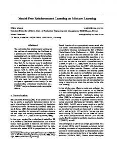
We comment on a decreasing step size. For a step size of the form εn = 1/nα , 0.5 < α ≤ 1, a similar analysis can be performed with ρn defined as ρn = nα/2 (θn − θ∗ ). In this case, θn converges to θ∗ w.p. 1, and the MSE decreases to zero at a rate O n−α/2 . Integrating a partial model in this case will reduce fluctuations in the converging path of the system. The performance gain of integrating a partial model is therefore more pronounced when the step size is constant. 4.3 Numerical Simulations of IPM-TD(0) We conclude this section with a demonstration of the performance of the IPM-TD(0) algorithm, and a comparison with the theory established above.8 Our simulations are on a set of abstract randomly constructed MDP’s termed Generalized Average Reward Non-stationary Environment Test-bench or in short GARNET (Bhatnagar et al., 2007). GARNET MDP’s comprise a class of randomly constructed finite MDP’s serving as a test-bench for RL algorithms. A GARNET MDP is characterized in our case by four parameters and is denoted by GARNET (|X | , |U | , B, σ). The parameter |X | is the number of states in the MDP, |U | is the number of actions, B is the branching factor of the MDP, that is, the number of uniformly distributed nonzero entries in each line of the MDP’s transition matrices, and the reward in each state is normally distributed with variance σ. For each GARNET MDP we also construct a ‘partially known’ MDP characterized by a parameter pK , 0 ≤ pK ≤ 1 such that each transition in the original MDP is known w.p. pK . The value of pK therefore indicates our level of knowledge about the MDP, ranging from no knowledge at all (pK = 0) up to knowing the complete MDP (pK = 1). For a GARNET(10, 5, 10, 1) MDP, a random deterministic policy was chosen and its value function was evaluated using algorithm (17). The error kθKn − θ∗ k2 , averaged over 500 different runs with the same initial conditions, is plotted in Figure 1 (left) for different values of pK . The asymptotic MSE was calculated using (23) and is shown for comparison. In Figure 1 (middle), the step size for an iteration with partial knowledge was set such that the asymptotic MSE would match that of the iteration without partial knowledge. As can be seen, this caused the IPM iteration to converge faster. For the next simulation a linear FA was used, with basis vectors φ(x) ∈ {0, 1}L , where the number of nonzero values in each φ(x) is l. The nonzero values were chosen uniformly at random, with any two states having different feature vectors. Figure 1 (right) shows the error kθKn − θ∗ k2 for a GARNET(30, 5, 10, 1) MDP, where we used linear FA with L = 10 and l = 2. As can be seen, the behavior observed in the tabular case is characteristic of the FA case as well.

5. Inaccuracy of the Partial Model Until now, we have assumed that our partial model contained accurate probability ratios. Obviously, such a strong assumption is not realistic, and in any practical situation our partial knowledge would contain some degree of error. In this section we consider the effect of inaccuracies in the partial model on the performance of the IPM-TD(0) method. Specifically, our goal is to show that if the inaccuracy in the partially known model is small enough, then an improvement in performance over regular TD(0) can still be guaranteed, and we seek bounds on the error in the algorithm induced by the inaccuracy in the model. Before we go into mathematical detail we first describe our conceptual approach. 8. The code for generating the results presented here can be found at the author’s web site.

1940


2

25 pk = 0

pk = 0.3

pk = 0.5

pk = 0.5

1.5

2

pk = 0 20

p =0 p = 0.3

1.6

p = 0.5

k k

p = 0.8

pk = 0.8

k

1.4

15

MSE

MSE

k

1.8

1 10

1.2 1

0.5

0.8

5 0.6

0

0

100

200

300

400

Iteration

500

600

0

0

100

200

300

400

500

600

700

0.4

0

50

Iteration

100

150

200

250

Iteration

Figure 1: TD(0) with a Partial Model. Left : MSE of Table Based IPM-TD(0) on a GARNET(10,5,10,1) MDP with a deterministic random policy, for different values of pK . Step size is ε = 0.2. Dashed lines show the asymptotic MSE calculated by (23). Middle : MSE of Table Based IPM-TD(0) on a GARNET(10,5,10,1) MDP with a deterministic random policy. For pK = 0 (black-solid) a step size ε = 0.15 was used, and the asymptotic MSE was calculated using (23) (black-dashed). For pK = 0.5 (red-solid) a step size was calculated (using (23)) such that its asymptotic MSE would equal that of pK = 0. Right : MSE of linear FA IPM-TD(0) on a GARNET(30,5,10,1) MDP with a deterministic random policy, for different values of pK . Step size is ε = 0.15. The linear FA parameters are L = 10 and l = 2. A discount factor of γ = 0.7 was used in all simulations. All results are averaged over 500 different runs with the same initial conditions. Error bars display the standard error of the mean; for clarity of presentation the bars are displayed only for the last iteration.

A key point in the analysis of IPM-TD(0) in Section 4 was that since the estimator µˆ K in (5) is unbiased, then the ODE of the stochastic approximation does not change, and asymptotically the algorithm concentrates around its fixed point which is the true value function. This is no longer valid when the partial model is not accurate, as the inaccuracy induces a bias in µˆ K . Since we use the estimator at every time step, this bias may accumulate, and the crucial question here is how it affects the algorithm asymptotically, and whether it can be guaranteed that small model errors do not cause a large deviation from the true value function. The improvement in performance of IPM-TD(0) relied on the variance reduction property of µˆ K . We shall see that if the inaccuracy in the partial model is small enough, then this property can still be guaranteed. Thus, our analysis consists of investigating the bias and the variance of IPM-TD(0) with an inaccurate model. As we have done earlier, we first describe some results in the context of estimating the mean of a random variable, and later extend the results to the MDP setting. 5.1 Estimation of a Random Variable Mean Consider the definitions of Section (2), and let Pˆ (ω) ω∈Ω denote inaccurate probabilities, obtained by some means. For some ε > 0 we define an ε−known set K ε by K ε , ω : ω ∈ Ω s.t. PˆKε (ω) − PKε (ω) < ε , 1941

(26)


where the probability measures PˆKε and PKε are defined by PˆKε (ω) , Pˆ (ω) / ∑ Pˆ (ω′ ) and PKε (ω) , ω′ ∈K ε

ˆ Kε [·] the expectation and variance P (ω) / ∑ P (ω′ ), respectively. Also denote by Eˆ Kε [·] and Var ω′ ∈K ε

under the measure PˆKε , and by EKε [·] and VarKε [·] the expectation and variance under the measure PKε . n We motivate the definition of the ε−known set with an example. Let xi i=1 denote i.i.d. samples of X. For some set K ⊂ Ω let PˆK (ω) denote the count ratios in K n  ∑ 1(xi =ω)   i=1 for ω ∈ K n , PˆK (ω) = ∑ 1(xi ∈K) i=1    0 else where 1 is the indicator function. It can be shown that PˆK (ω) is an unbiased estimate of PK (ω), and by the law of large numbers we have that for large n, the difference PˆK (ω) − PK (ω) is small. Furthermore, for a finite n, Chernoff type bounds can be used to bound this difference with high probability by some small ε, motivating definition (26). An estimator for µ that uses the ε−known set is derived by plugging K ε instead of K in (5) ε ε µˆ Kε (x) = 1Kx Eˆ Kε [X] + 1Kx¯ x.

(27)

Note that since the known set is not accurate, the estimator (27) is no longer unbiased. The following theorem, which we prove in Appendix C, bounds the bias and variance of µˆ Kε (x). Theorem 9 The bias of µˆ Kε (x) satisfies |E [ˆµKε (X)] − E [X]| ≤ εP (K ε )

∑ |x| .

x∈K ε

The variance of µˆ K ε (x) satisfies Var [ˆµKε (X)] ≤ Var [X] − P (K ε ) · VarKε [X]  !

(28)

2

ε

+εP (K ) ε

∑ |x|

x∈K ε

+2

∑ |x|

x∈K ε

!



|EK ε [X] − E [X]| .

5.2 Error Bound for IPM-TD(0) We now derive asymptotic error bounds for IPM-TD(0) with a constant stepsize ε˜ , when the partial model is inaccurate. We treat only the table based algorithm θn+1 (xn ) = θn (xn ) + ε˜ dnK , ε ¯ε θn (xn+1 ) − θn (xn ), dnK , r (xn ) + γ 1Kn+1 Eˆ Kεxn [ θn (xn+1 )| xn ] + 1Kn+1

(29)

where Eˆ Kεxn [ θn (xn+1 )| xn ] denotes expectation under the probability measure in the ε−known set Kxεn       Pˆ ( y| x) P ( y| x) ε < ε . (30) Kx , y : y ∈ X s.t. −   ∑ Pˆ ( y′ | x) P ( y′ | x) ∑   y′ ∈K ε y′ ∈K εx x

1942


The ODE for (29) can be written as dθ = Π (r + (γ (P + δP) − I) θ) , dt where δPi j =

   

! ∑ P ( k| i) 

k∈K εi

   0,

ˆ j|i) P( ˆ k|i) ∑ P(

k∈K εi

−

(31) 

P( j|i)  , ∑ P( k|i)

k∈K εi

j ∈ Kiε ,

(32)

j∈ / Kiε .

Recalling that the true value function satisfies θ∗ = (I − γP)−1 r, the asymptotic limit point of the ODE (31) is denoted by θ∗ + δθ , and satisfies θ∗ + δθ = (I − γ (P + δP))−1 r.

(33)

In the next subsection we show how to bound the error term δθ. 5.2.1 A B OUND

ON THE

B IAS

We would like to bound the term δθ, which is the error in the value function, and can be seen as the total bias induced by the IPM method with the inaccurate model. Note that (33) describes a perturbed linear system (Horn and Johnson, 1985, §5). Using tools for dealing with such systems, we can bound the error as presented in the following theorem. ε Theorem 10 Let Kmax denote the cardinality of the largest ε−known set Kxε , ε Kmax = max |Kxε | ,

(34)

x

and let ε satisfy ε
1 − γ,

since P is stochastic and thus its largest eigenvalue is 1. Using (39) we therefore have kγδPk∞ γK ε ε ≤ max . kI − γPk∞ 1−γ

We now bound κ (I − γP) = kI − γPk∞ (I − γP)−1 . First, by the triangle equality we have ∞

kI − γPk∞ ≤ kIk∞ + γ kPk∞ = 1 + γ,

(40)

since P is a stochastic matrix and by definition (38) we have kPk∞ = 1. Next we have by definition of the induced norm

1

−1 −1 , (41)

(I − γP) = max (I − γP) r ≤ 1−γ ∞ ∞ krk∞ =1 since (I − γP)−1 r can be seen as the value function associated with a reward vector r, which can have a maximum value of rmax / (1 − γ). From (40) and (41) we have 1+γ κ (I − γP) ≤ . 1−γ

All is left is to verify that (I − γP)−1 kγδPk∞ < 1. Using (39) and (41) this is satisfied if ∞

ε
0 .

The possible controls are to accept or reject a call, denoted by u ∈ {ua , ur }, respectively, and the immediate reward is ( c (m) if u = ua , ω (m) = 1, (s + ω, ω) ∈ X , r (x, u) = 0 else. The goal is to find the optimal policy with respect to the the average reward η = E[r(x)]. 11. We note that a learning policy may be required even when the model is fully known, as finding the optimal policy is often an intractable problem. This ’fully known’ scenario may be seen as a special case of the following presentation.

1947


6.1.3 T RANSITION P ROBABILITIES In order to transform the continuous time process into discrete transitions between events, a uniformization technique (Gallager, 1995, §6.4) is used. Define z to be the maximal transition rate, given by ( ) M

z = max x∈X

∑ (α (m) + s (m) β (m))

.

(44)

m=1

For a state x = (s, ω), the probability that the next event is an arrival of a call of type m is equal to α (m) /z. The probability for a departure of a call of type m is β (m) s (m) /z. By normalization, the M

probability that in the next event nothing happens is 1 − ∑ (α (m) + s (m) β (m)) /z. m=1

6.1.4 PARTIALLY K NOWN MDP For this problem, a natural definition for partial model knowledge is through the arrival and departure rates α, β, namely MK , {m : m ∈ 1, . . . , M s.t. α (m) , β (m) are known} . As an example where such partial knowledge arises in practice, consider a case where new jobs (with unknown rates) are added to an existing system (with previously known rates). Note that generally, the values in MK do not suffice for calculating z in (44), hence the transition probabilities of the MDP are not known. Nevertheless, the key point here is that in the ratios between transition probabilities, the z terms cancel out, therefore the partial MDP definition (11) can be satisfied. In particular, letting i ∈ MK , we have α (i) P (arrival of type i) = , ∑ P (arrival of type j) ∑ α ( j) j∈MK

j∈MK

and similar expressions hold for probabilities of departures. 6.1.5 IPM Q-L EARNING The model free RL algorithm we use for this problem is a variant of the popular Q-Learning algorithm for average return.12 For each state-action pair, a Q value is maintained, and updated according to ! 1 Qn xn+1 , u′ − Qn (xn , un ) − Qn+1 (xn , un ) = Qn (xn , un ) + εn r (xn , un ) + max Qn (x, u) . |X | |U | ∑ u′ x,u (45) The greedy deterministic policy u (x) w.r.t. the Q values at time n is u (x) = argmaxQn x, u′ . u′

Update (45) is an SA, and was shown to converge (Abounadi et al., 2001) under suitable step sizes εn to a fixed point Q∗ , such that the greedy policy w.r.t. Q∗ is optimal. Applying the IPM method in 12. This is also known as relative value iteration.

1948


Call Type m α (m) β (m) b (m) c (m)

1 1.8 0.4 1 1.4

2 1.4 0.7 1 1

3 1.6 0.5 1 1.6

4 1.4 0.4 1 1

Table 1: Call Types Qn (xn+1 , u′ ) in (45) with this case simply amounts to replacing max ′ u

1Kn+1 ·

Qn (y, u′ ) ∑ Pun (y|xn )max ′ u

y∈Kxn ,un

∑ Pun (y|xn )

¯ ′ x , u . · max Q + 1Kn+1 n+1 n ′ u

y∈Kxn ,un

(46)

We now report on the results of using IPM Q-learning for optimizing a call admission control policy. 6.1.6 R ESULTS In our experiments, we consider a link with a bandwidth of 7 units, and 4 call types. The parameters for each call are summarized in Table 1, and the size of the state space in this configuration is |X | = 2490. IPM Q-Learning was run with initial values Q0 (x, u) = r (x, u) and a step size εn = γ0 / (γ1 + vn (xn , un )) , where vn (x, u) denotes the number of visits to the state action pair (x, u) up to time n. The values of γ0 , γ1 were manually tuned for optimal performance, and set to γ0 = γ1 = 40. The action selection policy while learning was ε − greedy, with ε = 0.1. The partial model for each experiment is represented by a single parameter k, such that the arrival and departure rates of all calls of type m ≤ k are known. Figure 2 shows the average reward η as a function of iteration. As can be seen, incorporation of partial model knowledge by the IPM method resulted in a significant performance improvement. 6.2 IPM Policy Gradient In this experiment simulations were performed on randomly generated MDP’s, as described in Section 4.3. In the experiments, the agent maintains a stochastic policy function parametrized by θ ∈ RL·|U | , and given by T T ′ µθ (u|x) = eθ ξ(x,u) / ∑ eθ ξ(x,u ) , u′

where the state-action feature vectors ξ(x, u) ∈ {0, 1}L·|U | are constructed from the state features φ(x) defined in Section 4.3 as follows ξ(x, u) , (0, ...(L × (u − 1) zeros), φ(x), 0, ...(L × (|U | − u) zeros))T . The agent’s goal is to find the parameter θ which maximizes the average reward η = E[r(x)]. Policy Gradient algorithms achieve this goal by estimating the gradient w.r.t. θ of the average reward, ∇θ η, and performing a stochastic gradient ascent on the parameters to reach a local maximum. One such algorithm was proposed by Marbach and Tsitsiklis (1998). At time n we update the parameter vector θ and a scalar λ which is an estimate of η, 1949


0.354 k=0 k=2 k=3

0.352 0.35

average reward

0.348 0.346 0.344 0.342 0.34 0.338 0.336 0.334

0

1

2

3

4

iteration

5 5

x 10

Figure 2: IPM Q-Learning for Admission control. Implementation of IPM Q-Learning, (45) and (46), for the call admission control problem of Table 1. Average reward of the greedy policy is plotted vs. iteration number for different values of k. Results are averaged over 100 different runs with the same initial conditions. Error bars display the standard error of the mean; for clarity of presentation the bars are displayed only for the last iteration.

θn+1 = θn + ε (r (xn ) − λn ) zn , ′

λn+1 = λn + ε (r (xn ) − λn ) ,

(47) (48)

where ε and ε′ are step sizes, and ε′ < ε. We then simulate a transition to the next state, and update the vector z by zn+1 = zn + Lxn ,un (θn ) , where Lxn ,un (θn ) is the likelihood ratio Lx,u (θ) = ∇θ log µθ (u|x). Every time a predefined recurrent state of the MDP is visited, zn+1 is reset to zero. Denote by 1Kn an indicator function that equals 1 if xn belongs to Kxn−1 ,un−1 and 0 otherwise. Incorporating partial knowledge into the algorithm using (12) simply amounts to replacing r (xn ) in (47-48) with ∑ K

1n ·

y∈Kxn−1 ,un−1

Pun−1 (y|xn−1 )r (y)

∑ y∈Kxn−1 ,un−1

Pun−1 (y|xn−1 )

+ 1Kn¯ · r (xn ) .

We simulated the policy gradient algorithm on a GARNET(30, 5, 10, 1) MDP. The state features were constructed as described in Section 4.3 with L = 10, l = 2. Figure 3 shows the average reward η as a function of iteration. These results indicate that the variance reduction in each iteration (guaranteed by Lemma 2) resulted, on average, in a better estimation of the gradient ∇θ η, and therefore a better policy at each step.

7. Discussion and Future Work Generally, when devising a solution to a difficult problem, one should incorporate into it all reliably available information. Model free RL algorithms typically operate without explicit knowledge of 1950


−0.1

Average Reward

−0.15

−0.2

−0.25

−0.3

−0.35

pk = 0 pk = 0.5

−0.4

−0.45

pk = 0.8 0

2

4

6

8

Iteration

10

12

14

16 4

x 10

Figure 3: Policy Gradient with a Partial Model. Implementation of the algorithm described in Section 6.2 on a GARNET(30,5,10,1) MDP, with step size parameters ε = 0.03 and ε′ = 0.003. The linear FA parameters are L = 10 and l = 2. Average reward is plotted vs. iteration number for different values of pK . Results are averaged over 500 different runs with the same initial conditions. Error bars display the standard error of the mean; for clarity of presentation the bars are displayed only for the last iteration.

the underlying environment, and therefore, when such knowledge is available, using these algorithms ‘out of the box’ is clearly suboptimal. In this work we have presented a general method of integrating partial environmental knowledge into a large class of model free algorithms. Our method improves the asymptotic behavior of the algorithm, and at each iteration reduces the estimation variance due to the uncertainty in the environment. We have proved mathematically (for TD(0)) and demonstrated in simulation (for Policy Gradient and Q-learning) an improvement in the algorithm’s overall performance. From a more conceptual point of view, we have shown that two distinct approaches to RL, the model free and the model based approaches, can be combined in such a way that gains from their respective merits. From this perspective, this work is just a first step towards a theoretical understanding of the combination of different RL approaches. A few issues are in need of further investigation. In this work we have not addressed the question of how the partially known model can be acquired. A number of possibilities come to mind. In a transfer learning or tutor learning settings, the partial model can come from an expert who has exact knowledge of a model that is partially similar. In a multi-agent setting with communication, information about different parts of the model can be gathered independently by each of the agents, and combined to create a partial model of the environment. An interesting possibility is to simultaneously gather information while adapting the policy using some model free algorithm. Using the SA algorithm (8), at the time of the n’th update of θ, we have already encountered a state-action trajectory of size n. Can we use this trajectory to construct an estimated partial MDP model, use it as in algorithm (12), and guarantee an improvement in the algorithm’s performance? This should be done with caution, since using the same trajectory for updating the parameter and the estimated model may cause overfitting. To see this consider the following example. Let {xi } be a sequence of normally distributed i.i.d. random variables with 1951


mean m, and assume that our goal is to estimate m. A natural approach is to use the empirical mean given by θn = 1n ∑ni=1 xi , which can also be calculated recursively using the following SA iterate θn+1 = θn +

1 (xn+1 − θn ) , n+1

(49)

θ0 = 0. One may hope, that by the time of the n’th update of θ we could use the n − 1 values of xi already observed to build a partial model for xn , and similarly to (12), use it to manipulate (49) in such a way that guarantees a performance improvement (in the estimation of m). However, it is known that for a normal distribution, the empirical mean is also the minimum variance unbiased estimator for m (Schervish, 1995). Our manipulation of (49) would therefore either add bias or increase the variance. Though this issue deserves careful analysis, we note that when a constant step size is used, the major influences on the current value of the parameter are the most recent measurements, thus older samples can be safely used to construct a partial model, mitigating the severity of this problem. Finally, we note that the IPM method adds to the algorithm a computational cost of O (Kmax ) evaluations of F (θn , xn , un , xn+1 ) at each iteration. In our experiments, this cost proved to be negligible in comparison to the computational cost of the simulator. However, if the computation of F (θn , xn , un , xn+1 ) is demanding, one may face a tradeoff between the performance of the resulting policy and the computational cost of obtaining it.

Acknowledgments The authors would like to thank Nahum Shimkin for helpful discussions.

Appendix A. Admissibility of µˆ K In this section, based on the definitions of Section 2, we address the following issue. Can a better estimator than µˆ K (x) be found? Since the MSE of any estimator, within a non-Bayesian setting, depends on the unknown µ, comparison of different estimators is a difficult task. A popular comparison framework is that of admissible estimators (Schervish, 1995). For a given known set K, an estimator is said to be admissible if there is no other estimator that achieves a smaller MSE for every distribution in PK (ω). Clearly, admissibility is a desirable property for an estimator, since an inadmissible estimator is guaranteed to be sub-optimal. The next theorem states that µˆ K is admissible. Theorem 15 The estimator µˆ K of (5) is admissible. Proof Let P˜ (ω) ∈ PK (ω) be defined as 1K P (ω) . P˜ (ω) = ω ∑ P (ω′ ) ω′ ∈K

For X ∼ P˜ (ω) it is clear that µˆ K (x) = E [X] for all x, therefore E [ˆµK (X) − µ]2 = 0, and no other estimator achieves a smaller MSE in this case.

1952


Appendix B. Proof of Lemma 5 Proof By the ergodicity of the Markov chain the joint probability for subsequent states is lim P (xn , xn+1 ) = P ( xn+1 | xn ) [π]xn .

n→∞

Now, observe that h i E (dn φ (xn )) (dn φ (xn ))T θn = θ∗ , xn

= Cov [ dn φ (xn )| θn = θ∗ , xn ] + E [ (dn φ (xn ))| θn = θ∗ , xn ] E [ (dn φ (xn ))| θn = θ∗ , xn ]T = γ2 φ (xn ) Cov φ(xn+1 )T θ∗ xn φ (xn )T + E [ dn φ (xn )| θn = θ∗ , xn ] E [ dn φ (xn )| θn = θ∗ , xn ]T ,

where the second equality follows from Cov [ dn φ (xn )| θn , xn ] = Cov dn φ (xn ) − r (xn ) + φ(xn )T θn θn , xn ,

since adding constants does not change the covariance. Using Lemma 1 and Lemma 2 we derive an expression for the IPM iteration h i E (dnK φ (xn )) (dnK φ (xn ))T θn = θ∗ , xn = γ2 φ (xn ) Cov φ(xn+1 )T θ∗ xn − P (Kx ) CovK φ(xn+1 )T θ∗ xn φ (xn )T + E [ dnK φ (xn )| θn = θ∗ , xn ] E [ dnK φ (xn )| θn = θ∗ , xn ]T h i = E (dn φ (xn )) (dn φ (xn ))T θn = θ∗ , xn − γ2 φ (xn ) P (Kx ) CovK φ(xn+1 )T θ∗ xn φ (xn )T .

We therefore have that

h i lim E (dn φ (xn )) (dn φ (xn ))T θn = θ∗ n→∞ h h ii = lim E E (dn φ (xn )) (dn φ (xn ))T θn = θ∗ , xn n→∞ h i = ∑ [π]x E (dn φ (xn )) (dn φ (xn ))T θn = θ∗ , xn

Σ0 =

x

= ΣK0 + γ2 ∑ [π]x φ (x) P (Kx ) CovK φ(x′ )T θ∗ x φ (x)T x

K

2

= Σ0 + γ

∑ [π]x φ (x) P (Kx ) Var x

K

φ(x′ )T θ∗ x φ (x)T .

Appendix C. Proof of Theorem 9 Proof First, observe that Eˆ Kε [X] − EKε [X] = ∑ x PˆKε (x) − PKε (x) ≤ ε ∑ |x| . x∈Kε x∈K ε 1953

(50)


Using (50) a simple bound on the bias of µˆ Kε is derived |E [ˆµKε (X)] − E [X]| = ∑ P (x) Eˆ K ε [X] − x x∈Kε = P (K ε ) Eˆ K ε [X] − EK ε [X] ≤ εP (K ε ) We now derive a bound on the MSE of µˆ Kε . h i 2 E (ˆµKε (X) − E [X])2 = ∑ P (x) Eˆ Kε [X] − E [X] + x∈K ε

∑ |x| .

x∈K ε

∑ P (x) (x − E [X])2

x∈K¯ ε

2 = P (K ε ) Eˆ Kε [X] − EKε [X] + EK ε [X] − E [X] + ∑ P (x) (x − E [X])2 x∈K¯ ε

≤ Var [X] − P (K ε ) · VarKε [X]  ! 2

+P (K ε )  ε ∑ |x|

+ 2ε

x∈K ε

∑ |x|

x∈K ε

!



|EK ε [X] − E [X]|

where in the inequality in the third line we used (50) and Lemma 2. We see that we have an 2 improvement in MSE terms if ε ∑ |x| + 2ε ∑ |x| |EK ε [X] − E [X]| < VarK ε [X], which is x∈K ε

x∈K ε

always satisfied as ε → 0. Similarly, for the variance we have h i h i E (ˆµK ε (X) − E [ˆµK ε (X)])2 = E (ˆµK ε (X) − E [X])2 − (E [ˆµK ε (X)] − E [X])2 ≤ Var [X] − P (K ε ) · VarK ε [X]  ! 2

+P (K ε )  ε ∑ |x| x∈K ε

+ 2ε

∑ |x|

x∈K ε

!



|EKε [X] − E [X]| .

Appendix D. Proof of Theorem 12 Note that without the δθ terms in (42), the bound on the variance for a random variable (28) could be used to compare [ΣK0 ]xx with [Σ0 ]xx . For small δθ, the difference in the variance should be small, as is proved in the following Lemma, which we first motivate with a simple example. Let X ∈ {1, 2} and X ′ ∈ {1 + η, 2 + η} be two random variables satisfying P(X = 1)=P (X ′ = 1+η) and P (X = 2) = P (X ′ = 2 + η). We expect that for small η, the difference between Var [X] and Var [X ′ ] should also be small. Lemma 16 Let X ∼ P (·) be a random variable over a finite set {Ωi }Ni=1 , where Ωi ∈ R. Let X ′ ∼ P (·) be a random variable over a finite set {Ω′i }Ni=1 , such that |Ωi − Ω′i | < η, i = 1, . . . , N. The variance of X ′ satisfies p Var X ′ ≤ Var [X] + η2 + 2η Var [X]. 1954


Proof First we have

since

h h 2 i 2 i Var X ′ = E X ′ − E X ′ ≤ E X ′ − E [X] , E

Next we have

h

2 i 2 X ′ − E [X] = Var X ′ + E X ′ − E [X] . E

h

2 i 2 X − E [X] = ∑P x′ x′ − E [X] , ′

x′

but since |Ωi − Ω′i | < η, ∀i then by the triangle equality we have |x′ − E [X]| ≤ |x − E [X]| + η, so we have h 2 i ≤ ∑P (x) (|x − E [X]| + η)2 E X ′ − E [X] x

= Var [X] + η2 + 2η∑P (x) |x − E [X]| x

p ≤ Var [X] + η + 2η Var [X], 2

where in the last inequality we used Cauchy–Schwartz under the expectation inner product: h|x − E [X]| , 1i2 ≤ h|x − E [X]| , |x − E [X]|i h1, 1i = Var [X] .

We now combine the result of Lemma 16 and the bound on the variance developed for the random variable (28) to prove Theorem 12. Proof (of Theorem 12) First, we use Lemma 16 to bound (42) i i h ε h ε ε ε Var 1K Eˆ K ε [θ∗ + δθ] + 1K¯ (θ∗ + δθ) ≤ Var 1K Eˆ Kε [θ∗ ] + 1K¯ (θ∗ ) 2η p +η2 + Var [θ∗ ], γ

ε ε and substitute [Σ0 ]xx = γ2 Var [θ∗ ]. We now use (28) to bound Var 1K Eˆ Kε [θ∗ ] + 1K¯ (θ∗ ) , which results in (43).

Appendix E. Proof of Theorem 4 As stated before, Theorem 4 is a consequence of Theorem 10.1.3 in Kushner and Yin (2003), for which a long set of assumptions is required. For the sake of clarity, this section is organized as follows. We first present a constrained version of the IPM-TD(0) algorithm and show that it converges weakly to a unique point. We then present some definitions needed for Theorem 10.1.3 in Kushner and Yin (2003), followed by an explicit statement of the theorem, without the required assumptions. Finally, we present the assumptions one by one, and prove that they are indeed fulfilled. 1955


E.1 Constrained Algorithm An important issue in the analysis of an SA algorithm (8) is the boundedness of the iterates. For many convergence results, a required condition is that the sequence θn be bounded almost surely. This condition is not trivial, and there are several approaches to satisfying it. One simple approach is to truncate the iterate θn when it leaves some prespecified constraint set denoted by H (Kushner and Yin, 2003). This will be done by introducing a ‘correction’ term Zn θn+1 = θn + εF (θn , xn , un , xn+1 ) + εZn ,

(51)

where εZn is the vector of shortest Euclidean length needed to take θn + εF (θn , xn , un , xn+1 ) back to the constraint set H if it is not in H. Respectively, the correction term needs to be added to the associated ODE dθ = g¯ (θ) + zt , (52) dt where zt maintains θ in H. Recall the unconstrained ODE for TD(0) (15), and its fixed point θ∗ . Since in TD(0) θ∗ is bounded by the maximal value of the MDP rmax / (1 − γ), we can choose H to be large enough such that θ∗ ∈ H. The following Lemma guarantees that in this case, the additional zt term in (52) does not change the ODE’s unique fixed point. Lemma 17 Assuming θ∗ ∈ H, the constrained ODE for IPM-TD(0) with linear function approximation dθ/dt = b + Aθ + zt , with b, A, zt defined in Section 4.1, has a unique and asymptotically stable fixed point θ∗ , which satisfies Aθ∗ = −b.

Proof Consider as a Lyapunov function the Euclidean distance to θ∗ , V (θ) = (θ − θ∗ )T (θ − θ∗ ). For the unconstrained ODE (10), we have13 V˙ (θ) = θT A + AT θ, and since A is negative definite we have V˙ (θ) < 0, and V (θ) is a valid Lyapunov function. Let V˙ H (θ) correspond to the constrained ODE. Since θ∗ is in H, by the geometric definition of the correction terms, we have V˙ H (θ) ≤ V˙ (θ) < 0, therefore V is also valid for the constrained ODE (52). We now state a convergence theorem that relates between the limit point of the ODE (52) and the asymptotic behavior of algorithm (51). The assumptions needed for this theorem are satisfied by default, by the definition of our RL environment and algorithm, and are thus omitted. Let θ (t) denote the piece-wise constant continuous time interpolation θn , where θ (t) = θn on the time interval [nε, nε + ε) for t ≥ 0 and θ (t) = θ0 for t < 0. Similarly define Z (t) as the piece-wise constant continuous time interpolation of Zn . Theorem 18 (Theorem 8.2.2 in Kushner and Yin, 2003) Consider algorithm (51). For any non decreasing sequence of integers qε , for each sub-sequence of {θ (εqε + ·) , Z (εqε + ·)} , ε > 0, there exist a further sub-sequence and a process (θ (·) , Z (·)) such that (θ (εqε + ·) , Z (εqε + ·)) ⇒ (θ (·) , Z (·)) as ε → 0 through the convergent sub-sequence, where θ (t) = θ (0) +

Zt

g¯ (θ (s)) ds + Z (t) .

0

Let εqε → ∞ as ε → 0. Then, for almost all ω, the path θ (ω, ·) lies in a limit set of (53). 13. See derivation in the proof of 20.3.3.

1956

(53)


E.2 Definitions The following technical definitions are required for the convergence result. Let DL (−∞, ∞) (and DL [0, ∞), respectively) denote the L−fold product space of real valued functions on the interval (−∞, ∞) (resp. on [0, ∞)) that are right continuous and have left-hand limits, with the Skorohod topology used.14 Let {qε } be a sequence of non-negative integers. In order to investigate the asymptotic behavior we will examine θ (εqε + ·), where εqε → ∞. We also demand ε (qε − pε ) → ∞ where pε are non decreasing and non-negative integers used in assumption 20.3. Define the normalized error process √ Un = (θqε +n − θ∗ ) / ε, and let U ε (·) denote its piecewise constant right continuous interpolation, with interpolation intervals ε, on [0, ∞). Define W ε (·) on (−∞, ∞) by  √ qε +t/ε−1   ∗  t ≥0  ε ∑ F (θ , xi , ui , xi+1 ) , i=qε ε W (t) = (54) √ qε +t/ε−1   ∗ − ε ∑ F (θ , xi , ui , xi+1 ) , t < 0  i=qε

E.3 A Theorem on Fluctuations in SA

Theorem 19 (10.1.3 in Kushner and Yin, 2003) Consider algorithm (51) and let assumption 20 hold. Then the sequence {U ε (·) ,W ε (·)} converges weakly in DL [0, ∞) × DL (−∞, ∞) to a limit denoted by {U (·) ,W (·)}, and dU = AUdt + dW, where the matrix A is defined in 20.8, W (·) is a Wiener process with covariance matrix Σ described in 20.5, and U (·) is stationary. Theorem 4 is a direct consequence of Theorem 19, with n = ω (1/ε) satisfying the requirement on qε . E.4 Assumptions for Theorem 19 The set of assumptions 20 which we describe in the following is designed to fit a wide variety of algorithms, and are thus quite complicated. The IPM-TD(0) algorithm with which we are concerned is a very simple case of this theorem, as it is linear, bounded, and stationary, and the Markovian state transitions are ergodic, and defined over a finite state space.15 Moreover, many of the assumptions that follow are used in order to reduce a more complicated algorithm to these simpler settings, and to show that the residual that remains is small in some sense. Thus, many complicated terms in the assumptions just vanish, and some assumptions are true by default. 14. See Kushner and Yin (2003, p. 228, 238) for more details on DL . 15. In Borkar (2008) a simpler result regarding fluctuations with a fixed step size is given, albeit for a martingale difference noise scenario. The Markovian state dependent noise in our case requires the more complicated approach of Kushner and Yin (2003).

1957


Assumption 20 The following holds16 1. F (θn , xn , un , xn+1 ) I{|θn −θ∗ |≤ρ} is uniformly integrable for small ρ > 0.

Proof F (θn , xn , un , xn+1 ) is uniformly integrable since on every sample path θn is bounded (by the constraint), r (xn ) is bounded by rmax and φ (xn ) is also bounded by definition. Since this is true for every sample path, F (θn , xn , un , xn+1 ) I{|θn −θ∗ |≤ρ} is uniformly integrable for all ρ.

2. There is a sequence of non-negative and non decreasing integers Nε such that θ (εNε + ·) converges weakly to the process with constant value θ∗ strictly inside the constraint set. Proof By the weak convergence Theorem 18, choosing Nε such that εNε → ∞, and by Lemma 17, we have that IPM-TD(0) converges weakly to the process with constant value θ∗ strictly inside the constraint set.

3. There are non decreasing and non-negative integers pε (that can be taken to be greater than Nε ) such that √ (θ pε +n − θ∗ ) / ε; ε > 0, n ≥ 0 is tight.

Proof For the proof of this assumption we use Theorem 10.5.2 in Kushner and Yin (2003), which we now state. Theorem 21 (10.5.2 in Kushner and Yin, 2003) Assume the constrained algorithm 51 with constraint set H, where θ∗ is in the interior of H. Assume that 20.2 and 20.3.1-20.3.7 hold in √ H. Then there are pε < ∞ such that (θ pε +n − θ∗ ) / ε; ε > 0, n ≥ 0 is tight.

3.1 θ∗ is a globally asymptotically stable (in the sense of Lyapunov) point of the ODE dθ/dt = g¯ (θ) + zt . Proof This is satisfied by Lemma 17.

3.2 The non-negative and continuously differentiable function V (·) is a Lyapunov function for the ODE. The second order partial derivatives are bounded and |∇θV (θ)|2 ≤ K1 (V (θ) + 1), where K1 is an arbitrary positive number. Proof Choose V to be of the form V (θ) = (θ − θ∗ )T (θ − θ∗ ). As was in the proof of Lemma 17, V is a valid Lyapunov function. The second order partial derivatives are zero, and ∇θV (θ) = 2 (θ − θ∗ ) 16. We exclude assumptions which are true by definition of our RL settings.

1958


|∇θV (θ)|2 = 4 |θ − θ∗ |2 = 4V (θ) .

3.3 There is a λ > 0 such that VθT (θ) g¯ (θ) ≤ −λV (θ) Proof Recalling from (15) and (16) that g¯ (θ) = b + Aθ, we have

T 1 = (θ − θ∗ )T (b + Aθ) + (b + Aθ)T (θ − θ∗ ) (∇θV (θ))T g¯ (θ) + (∇θV (θ))T g¯ (θ) 2 = (θ − θ∗ )T b + bT (θ − θ∗ )

+ (θ − θ∗ )T Aθ + θT AT (θ − θ∗ )

= (θ − θ∗ )T b + bT (θ − θ∗ ) + (θ − θ∗ )T A + AT (θ − θ∗ )

+ (θ − θ∗ )T Aθ∗ + θ∗T AT (θ − θ∗ )

= (θ − θ∗ )T (b + Aθ∗ ) + (b + Aθ∗ )T (θ − θ∗ ) + (θ − θ∗ )T A + AT (θ − θ∗ ) = (θ − θ∗ )T A + AT (θ − θ∗ ) .

Let λ′ denote the largest eigenvalue of A + AT . We have that (θ − θ∗ )T A + AT (θ − θ∗ ) ≤ λ′ (θ − θ∗ )T (θ − θ∗ ), and (∇θV (θ))T g¯ (θ) = (θ − θ∗ )T A + AT (θ − θ∗ ) ≤ λ′V (θ) .

3.4 For each K > 0, supE |F (θn , xn , un , xn+1 )|2 I{|θn −θ∗ |≤K} ≤ K1 E [V (θn ) + 1], where K1 does not n

depend on K. Proof Satisfying this requirement is immediate, since F (θn , xn , un , xn+1 ) is bounded on every sample path. This follows from the fact that on every sample path θn is bounded (by the constraint), r (xn ) is bounded by rmax and φ (xn ) is also bounded by definition. ∞

3.5 The sum Γn (θ) = ε ∑ (1 − ε)i−n En [g (θ, xi , ui ) − g¯ (θ)], where En denotes expectation condii=n

tioned on the history up to time n, is well defined in that the sum of the norms of the summands is integrable for each θ, and E |Γn (θn )|2 = O ε2 . Proof From Lemma 6.7 in Bertsekas and Tsitsiklis (1996) (which relies on the exponential mixing time of Markov chains) we have that |En [g (θ, xi , ui ) − g¯ (θ)]| ≤ cρi−n |θ| for some 1959


c > 0 and ρ < 1. This gives ∞ i−n (1 − ε) E [g (θ, x , u ) − g ¯ (θ)] ∑ ≤ n i i i=n

≤

=

∞

∑ |En [g (θ, xi , ui ) − g¯ (θ)]|

i=n ∞

∑ cρi−n |θ|

i=n

c |θ| , 1−ρ

and E |Γn (θn )|

2

c |θn | 2 ≤ ε E 1−ρ ε2 c ∗ 2 |θ | = 1−ρ = O ε2 . 2

3.6 E |Γn+1 (θn+1 ) − Γn+1 (θn )|2 = O ε2 . Proof

We have

Γn+1 (θn+1 ) − Γn+1 (θn ) ∞

= ε

∑

i=n+1 ∞

−ε

(1 − ε)i−n−1 En+1 [g (θn+1 , xi , ui ) − g¯ (θn+1 )]

∑

i=n+1 ∞

= ε

∑

i=n+1

(1 − ε)i−n−1 En+1 [g (θn , xi , ui ) − g¯ (θn )]

(1 − ε)i−n−1 En+1 [g (θn+1 , xi , ui ) − g (θn , xi , ui ) − (g¯ (θn+1 ) − g¯ (θn ))] .

Using the triangle inequality |Γn+1 (θn+1 )−Γn+1 (θn )| ≤ ∞

ε

∑ (1 − ε)i−n−1 |En+1[g (θn+1 , xi , ui )−g (θn , xi , ui )−(g¯ (θn+1 )−g¯ (θn ))]|

i=n+1

By the linearity of g, g, ¯ and since θn is bounded, we have that|g (θn+1 , xi , ui ) − g (θn , xi , ui )| < ¯ for some k. ¯ We therefore have : kε for some k, and |g¯ (θn+1 ) − g¯ (θn )| < kε |En+1 [g (θn+1 , xi , ui ) − g (θn , xi , ui )]| ≤ En+1 [|g (θn+1 , xi , ui ) − g (θn , xi , ui )|] < kε, 1960


and similarly ¯ |En+1 [g¯ (θn+1 ) − g¯ (θn )]| < kε. Now |Γn+1 (θn+1 ) − Γn+1 (θn )| ≤ ε2 k + k¯

∞

∑

i=n+1

(1 − ε)i−n−1

= ε k + k¯ ,

and

2 |Γn+1 (θn+1 ) − Γn+1 (θn )|2 ≤ ε2 k + k¯ = O ε2 .

3.7 Let θH denote the projection of θ onto H. Then for all θ, V θH ≤ V (θ). Proof This assumption was shown to hold in the proof of Lemma 17.

4. For a small ρ > 0, and any sequence ε → ∞ and n → ∞ such that θn → θ∗ in probability, i h E |δMn − δMn (θ∗ )|2 I{|θn −θ∗ |≤ρ} → 0. Proof Recall that we have δMn = E [ dnK φ (xn )| xn , un ] − dnK φ (xn ) = γ∑Pun ( y| xn ) φ(y)T θn φ (xn ) y



∑ Pun ( y| xn ) φ(y)T

y∈Kxn ,un  −γ 1Kn+1 ∑ Pun ( y| xn ) y∈Kxn ,un





 ¯ φ(xn+1 )T  θn φ (xn ) + 1Kn+1

∑ Pun ( y| xn ) φ(y)T

y∈Kxn ,un  = γ ∑Pun ( y| xn ) φ(y)T − 1Kn+1 ∑ Pun ( y| xn ) y y∈Kxn ,un

The difference δMn − δMn (θ∗ ) can therefore be written as



 ¯ φ(xn+1 )T  θn φ (xn ) . − 1Kn+1

δMn − δMn (θ∗ ) = a (xn )T (θn − θ∗ ) b (xn ) , where a and b are vector valued functions of xn . By the Cauchy–Schwarz inequality, for every xn |δMn − δMn (θ∗ )| ≤ |a (xn )| |θn − θ∗ | |b (xn )| , 1961


and since the state space is finite, a and b are bounded, therefore there exists some constant k such that for every xn |a (xn )| |b (xn )| ≤ k, and we have that i h E |δMn − δMn (θ∗ )|2 I{|θn −θ∗ |≤ρ} ≤ k2 |θn − θ∗ |2 → 0.

5. The sequence of processes W (·) defined on (−∞, ∞) by (54) converges weakly in DL (−∞, ∞) to a Wiener process W (·), with covariance matrix Σ. Proof For the proof of this assumption we use Theorem 10.6.2 in Kushner and Yin (2003),which we now state. Theorem 22 (10.6.2 in Kushner and Yin, 2003) Assume 20.5.1-20.5.4. Then {W (·)} defined in (54) converges weakly to a Wiener process with covariance matrix Σ = Σ0 + Σ1 + ΣT1 .

5.1 The following equations hold:

Proof

∞ lim supE ∑ E F (θ∗ , x j , u j , x j+1 ) xn , un = 0, N→∞ n j=n+N ∞ lim supE ∑ E ( F (θ∗ , xn , un , xn+1 ) F (θ∗ , xi , ui , xi+1 )| xn , un )T = 0. N→∞ n i=n+N

Since the transition probabilities at step j converge to the steady state transition probabilities (a property of ergodic Markov chains) exponentially fast in j, and since at the steady state E (F (θ∗ , x, u, x′ )) ≡ g¯ (θ∗ ) = 0, we have that for some ρ < 1 and some vector c E F (θ∗ , x j , u j , x j+1 ) xn , un < cρ j−n , therefore for every n

∞ ∗ lim ∑ E F (θ , x j , u j , x j+1 ) xn , un ≤ N→∞ j=n+N

=

∞

lim c ∑ ρ j

N→∞

lim

N→∞ 1 − ρ

= 0. 1962

j=N cρN


The same goes for the covariance, since there exists some ρ′ < 1 and some matrix c′ such that E ( F (θ∗ , xn , un , xn+1 ) F (θ∗ , xi , ui , xi+1 )| xn , un )T < c′ ρ′i−n .

o n 5.2 The sets |F (θ∗ , xn , un , xn+1 )|2 and tegrable.

( 2 ) ∞ ∑ E F (θ∗ , x j , u j , x j+1 ) xi , ui are uniformly in j=i

o n Proof As was shown before, F (θ∗ , xn , un , xn+1 ) is bounded, and therefore |F (θ∗ , xn , un , xn+1 )|2 is uniformly integrable. Also, as was shown in the proof of A5.1, for every i ∞ c , ∑ E F (θ∗ , x j , u j , x j+1 ) xi , ui ≤ 1−ρ j=i ( ) ∞ 2 ∗ which is bounded, and therefore ∑ E F (θ , x j , u j , x j+1 ) xi , ui is uniformly integrable. j=i 5.3 There is a matrix Σ0 such that i 1 n+m−1 h T ∗ ∗ x , u E F (θ , x , u , x ) F (θ , x , u , x ) j j j+1 j j j+1 n n − Σ0 → 0 ∑ m j=n

in probability as n, m → ∞. Proof

Since the Markov chain is ergodic, by the law of large numbers this is satisfied by defining h i Σ0 = lim E F (θ∗ , xn , un , xn+1 ) F (θ∗ , xn , un , xn+1 )T . n→∞

5.4 There is a matrix Σ1 such that i h 1 n+m−1 ∞ T ∗ ∗ E F (θ , x j , u j , x j+1 ) F (θ , xk , uk , xk+1 ) xn , un − Σ1 → 0 ∑ ∑ m j=n k= j+1

in probability as n, m → ∞. Proof

Since the Markov chain is ergodic, by the law of large numbers this is satisfied by defining h i ∞ Σ1 = ∑ lim E F (θ∗ , xn , un , xn+1 ) F (θ∗ , xn+ j , un+ j , xn+ j+1 )T . n→∞ j=1

1963


6. g (·, x, u) is continuously differentiable for each x, u, and can be expanded as g (θ, x, u) = g (θ∗ , x, u) + [∇θ g (θ∗ , x, u)]T (θ − θ∗ ) + [y (θ, x, u)]T (θ − θ∗ ) , where [y (θ, x, u)]T (θ − θ∗ ) =

Z 1 0

[∇θ g (θ∗ + s (θ − θ∗ ) , x, u) − ∇θ g (θ∗ , x, u)] ds,

(55)

and if δ → 0 as ε → 0 and n → ∞, then E |y (θn , xn , un )| I{|θn −θ∗ |≤δ} → 0 as ε → 0 and n → ∞. Proof Recall that for IPM-TD(0) T

r (x) + γ∑Pu ( y| x) φ(y) − φ(x)

g (θ, x, u) =

T

y

! !

θ φ (x) ,

which is linear in θ and thus can be expanded as g (θ, x, u) =

T

r (x) + γ∑Pu ( y| x) φ(y) − φ(x) y

∗

T

!

T

∗

!

(θ − θ + θ ) φ (x)

= g (θ , x, u) + γ∑Pu ( y| x) φ(y) − φ(x) y

∗

T

!

(θ − θ∗ ) φ (x)

= g (θ , x, u) + [∇θ g (θ∗ , x, u)]T (θ − θ∗ ) . ∗

Since ∇θ g (θ, x, u) does not depend on θ, the integral in (55) is zero and y (θ, x, u) = 0, thus the assumption is satisfied.

7. The set {∇θ g (θ∗ , xn , un )} is uniformly integrable.

Proof As was shown above, ∇θ g (θ∗ , xn , un ) is clearly bounded, and therefore uniformly integrable.

8. There is a Hurwitz matrix A such that 1 n+m+1 E ∇θ gT (θ∗ , x j , u j ) xn , un − A → 0 ∑ m j=n

in probability as ε → 0 and n, m → ∞.

1964


Proof We have, ∇θ gT (θ∗ , x, u) = φ(x) γ ∑Pu ( y| x) φ(y) − φ(x) y

!T

.

Recall our definition of A A , ΦT Πµ (γPµ − I) Φ. Then, by the law of large numbers, we have 1 n+m+1 E ∇θ gT (θ∗ , xi , ui ) xn , un − A → 0. ∑ m j=n

As was stated before, it can be shown (Bertsekas and Tsitsiklis, 1996, Lemma 6.6b) that the eigenvalues of A all have a negative real part, therefore A is Hurwitz.

References P. Abbeel, M. Quigley, and A.Y. Ng. Using inaccurate models in reinforcement learning. In Proceedings of the 23rd International Conference on Machine Learning, pages 1–8. ACM, 2006. J. Abounadi, D. Bertsekas, and V.S. Borkar. Learning algorithms for markov decision processes with average cost. SIAM Journal on Control and Optimization, 40(3):681–698, 2001. A.G. Barto, S.J. Bradtke, and S.P. Singh. Learning to act using real-time dynamic programming. Artificial Intelligence, 72(1-2):81–138, 1995. D.P. Bertsekas. Dynamic Programming and Optimal Control, Vol I & II. Athena Scientific, third edition, 2006. D.P. Bertsekas and J. Tsitsiklis. Neuro-dynamic Programming. Athena Scientific, 1996. S. Bhatnagar, R. Sutton, M. Ghavamzadeh, and M. Lee. Natural actor–critic algorithms. Technical Report TR09-10, Univ. of Alberta, 2007. V.S. Borkar. Stochastic Approximation: a Dynamical Systems Viewpoint. Cambridge University Press, 2008. R.I. Brafman and M. Tennenholtz. R-max a general polynomial time algorithm for near-optimal reinforcement learning. The Journal of Machine Learning Research, 3:213–231, 2003. R. Crites and A. Barto. Improving elevator performance using reinforcement learning. In Advances in Neural Information Processing Systems 8, pages 1017–1023. MIT Press, 1996. N.D. Daw, Y. Niv, and P. Dayan. Uncertainty-based competition between prefrontal and dorsolateral striatal systems for behavioral control. Nature Neuroscience, 8(12):1704–1711, 2005. 1965


P. Dayan and T.J. Sejnowski. TD(λ) converges with probability 1. Machine Learning, 14:295–301, 1994. R.G. Gallager. Discrete Stochastic Processes. Kluwer Academic Publishers, 1995. R. A. Horn and C. R. Johnson. Matrix Analysis. Cambridge University Press, 1985. M. Kearns and S. Singh. Near-optimal reinforcement learning in polynomial time. Machine Learning, 49(2):209–232, 2002. V. Konda. Actor-Critic Algorithms. PhD thesis, Massachusetts Institute of Technology, 2002. P.R. Kumar. A survey of some results in stochastic adaptive control. SIAM Journal on Control and Optimization, 23:329–380, 1985. H.J. Kushner and G. Yin. Stochastic Approximation and Recursive Algorithms and Applications. Springer Verlag, 2003. L. Ljung. Analysis of recursive stochastic algorithms. IEEE Transactions on Automatic Control, 22 (4):551 – 575, 1977. P. Marbach and J. Tsitsiklis. Simulation-based optimization of markov reward processes. IEEE Transactions on Automatic Control, 46(2):191–209, 1998. P. Marbach, O. Mihatsch, M. Schulte, and J.N. Tsitsiklis. Reinforcement learning for call admission control and routing in integrated service networks. In Advances in Neural Information Processing Systems 10, pages 922–928. MIT Press, 1998. A. Papoulis and S.U. Pillai. Probability, Random Variables, and Stochastic Processes. McGraw Hill, fourth edition, 2002. M.J. Schervish. Theory of Statistics. Springer, 1995. S. Singh and P. Dayan. Analytical mean squared error curves for temporal difference learning. Machine Learning, 32:5–40, 1998. R.S. Sutton. Integrated architectures for learning, planning, and reacting based on approximating dynamic programming. In Proceedings of the Seventh International Conference on Machine Learning, pages 216–224. Morgan Kaufmann, 1990. R.S. Sutton and A.G. Barto. Reinforcement Learning. MIT Press, 1998. G. Tesauro. Temporal difference learning and td-gammon. Commun. ACM, 38, March 1995.

1966

Integrating a Partial Model into Model Free Reinforcement Learning

Integrating a Partial Model into Model Free Reinforcement Learning

Suggest Documents

Model-Free Reinforcement Learning as Mixture Learning

A Reinforcement Learning Model of Reaching Integrating ... - PUMA

PAC Model-Free Reinforcement Learning - Semantic Scholar

A Generalized Reinforcement-Learning Model - Semantic Scholar

A neural-network reinforcement-learning model of

Reinforcement Learning Versus Model Predictive Control: A

A Reinforcement Learning Model Equipped with

Integrating a Usability Model into Model-Driven Web Development ...

Integrating a Usability Model into Model-Driven Web ... - UPV

Integrating e-learning into the Direct-instruction Model ...

The model of KM Learning Activities Integrating into ... - wseas.us

The model of KM Learning Activities Integrating into Business ...

Totally Model-Free Reinforcement Learning by Actor-Critic ... - CiteSeerX

Model-free Reinforcement Learning of Impedance Control ... - CiteSeerX

Model-free Reinforcement Learning of Impedance ... - Freek Stulp

PAC Model-Free Reinforcement Learning - University of California ...

Model-free off-policy reinforcement learning in continuous ... - CiteSeerX

Model-based hierarchical reinforcement learning and ... - BioMedSearch

An Environment Model for Nonstationary Reinforcement Learning

PAC-Bayesian Model Selection for Reinforcement Learning

Fuzzy Model-Based Reinforcement Learning - Semantic Scholar

Model-based Reinforcement Learning Approach for

Reinforcement Learning based Dynamic Model Selection for

Reinforcement Learning with Misspecified Model Classes