potential plant stress); spatial scales (e.g. association of soil and disease .... geographic and environmental) were assessed performing the Mantel test ... SDMtoolbox: a python-based GIS toolkit for landscape genetic, biogeographic and. 133.
Integrating GIScience and Crop Science datasets: a study involving genetic, geographic and environmental data
1
2
3
4
Roberto Santos1,2 , Adam Algar1 , Richard Field1 , and Sean Mayes3
5
1 School
6
2 Nottingham
of Geography, University of Nottingham, UK Geospatial Institute, University of Nottingham, UK 3 Plant and Crop Sciences, University of Nottingham, UK
7
ABSTRACT
8
9 10 11 12 13 14 15 16 17
Sharing and reusing data in research is a welcome and encouraged practice since it maximises the scientific outcomes given limited financial, material and human resources. Interdisciplinary research is considered to benefit from this practice, uniting researchers and data from two or more disciplines to advance fundamental understanding or tackle problems whose solution is beyond the limit of an individual body of knowledge. Here we discuss the challenges of combining data across disciplines, focusing in particular on associating geographic location data with genetic data in the context of a project involving Crop Science and Geospatial Information Science disciplines. This project aims to improve understanding of how geographical, environmental and anthropogenic factors affect the genetic variation in a neglected and underutilised crop called Bambara groundnut.
18
Keywords:
19
INTRODUCTION
20 21 22 23 24 25 26 27 28 29 30 31 32 33 34 35 36 37 38 39 40 41 42 43
Data integration, GIScience, Crop Science, Landscape Genetics, Bambara groundnut
Research challenges in the 21st century require an interdisciplinary approach, to advance fundamental understanding or to tackle problems whose solutions are beyond the scope of a single discipline or body of knowledge (Academies, 2004). Interdisciplinarity is encouraged, with funding organisations recently increasing support for research that integrates multiple disciplines. Interdisciplinary science represents the current reality for increasing numbers of scientists, through the composition of research teams and the nature of the hypotheses being examined (Dyer, 2015). In this context, sharing and reusing datasets from different disciplines is common practice and aims to strength the research by adding new dimensions to the data available or verifying the results obtained from a different perspective. However, integration of discipline-associated datasets is not a smooth process and is subject to varying concepts of quality and abundance. Geographic Information Science (GIScience) explores the location property of entities such as objects, events and processes, associating them with co-ordinates, such as longitude and latitude (Goodchild, 2010; Stevens and Pfeiffer, 2015). This process may seem straightforward, given the increasing presence of location-based sensors and mapping technologies in our daily lives. However, it is still a challenge because of the nature and contexts of the facts examined. In museums and herbaria, artefacts and specimens have usually been collected over decades or centuries and their finding location is often ambiguous or very imprecise (van Erp et al., 2015). In Health Science, investigation of historical records of disease occurrence in individuals relies on the names of locations and vague addresses. The lack of historical address databases undermines the potential use of those health data (Lash et al., 2012). In Crop Science, breeding programs rely on the collections of seeds available to germplasm banks. Knowledge about the origin of these seeds is necessary to characterise the environment around their collection location, and to go beyond basic measurements of diversity. However, again, location information about their origin may be vague or associated with markets where the seeds were obtained instead of where they grew or were originally sourced from (Richards, 2011).
PeerJ Preprints | https://doi.org/10.7287/peerj.preprints.2248v4 | CC BY 4.0 Open Access | rec: 26 May 2017, publ: 26 May 2017
44
A MODEL FOR INTEGRATION OF MULTIPLE DISCIPLINE DATA
76
In the cases just mentioned, integration of data from other disciplines with GIScience is not straightforward. In fact, the integration often involves transformation and filtering operations using arbitrary criteria. Given two datasets from different disciplines, these operations typically discard or reduce records or items, often greatly, resulting in a relative subset of the original dataset that can be used in both disciplines. In Figure 1, a Venn diagram shows this concept using three distinct disciplines. Given the initial amount of data in a discipline (D1), only a subset (D1 ∩ D2 or D1 ∩ D3) fits the criteria of both disciplines (D1 and D2 or D1 and D3). As the number of disciplines involved increases, so there is further diminution of the available data. These criteria involve requirements common and unique to the disciplines involved. Examples include the following cases: exclusion of records with missing data (i.e. records must have longitude and latitude or postcode); temporal scales (e.g. growing season must match respective weather data to investigate potential plant stress); spatial scales (e.g. association of soil and disease resistance among individuals in a small to medium farm demands detailed soil maps); sample units (e.g. if the location is available at the population level, the genetic information for individuals must be grouped by the same definition of the population). Another issue with integrating data from distinct disciplines concerns variation of concepts such as abundance and diversity. A dataset may fit criteria of relatively high abundance and diversity in discipline D1, but be classed as scarce and uniform in discipline D2. Figure 2A shows one seedling being planted in the glasshouse. In the context of Crop Science, this individual has the potential to generate a significant amount of genetic data through genotyping or sequencing processes (see figure 2C), and the resulting dataset could be considered abundant. However, genetic information among individuals of the same species can be very similar and in order to get data that represents the differences it is important to choose highly polymorphic molecular markers in the genotyping process. In the context of GIScience, this individual seedling, whose origin information is available at the population level, has only one associated location, and would be considered scarce if the objective were to analyse the genetic data over a broad geographic area. Even if more seedlings from the same population were cultivated (see figure 2B), the number of population locations is still one, and all the genetic data generated from these samples are still associated with one point in space (see figure 2D). Cultivating seeds from different populations would provide a better representation of the geographic space. However, it would be necessary to investigate the characteristics of interest around this location in order to guarantee a reasonable representation of environmental variables. Experiment design and sampling strategy are important, and should be discussed taking into account the characteristics of the data of the disciplines involved.
77
THE BAMBARA GROUNDNUT STUDY CASE
45 46 47 48 49 50 51 52 53 54 55 56 57 58 59 60 61 62 63 64 65 66 67 68 69 70 71 72 73 74 75
78 79 80 81 82 83 84 85 86 87 88
89 90 91 92 93 94 95
Bambara groundnut is classed as a neglected and underutilised species of legume, mainly cultivated in Sub-Saharan Africa. It is believed that the process of its domestication and further cultivation started thousands of years ago. However, despite its long history, this crop is still cultivated from landraces (locally developed mixtures of genotypes) (Molosiwa et al., 2015). The development of proper varieties of Bambara groundnut demands a better understanding of its genetic structure and diversity. Despite being a human-associated species cultivated in human-managed landscapes, we expected that the genetic resources of Bambara groundnut still have an influence of geographic and environmental factors. Initially, we mapped the results clustering analysis on the genetic data to explore potential spatial patterns of genetic variation. In the next step, we investigated the correlation between genetic, geographic and environmental by performing the Mantel test using three measures of distance among the samples. The next section includes a description of these analyses. The proposed pipeline We developed a pipeline to assimilate and analyse the genetic, geographic and environmental data using a mix open source tools such as Python, R and their respectively libraries and packages running in a Linux environment (see Figure 3). By adopting open source software in our project, we pursued a set of best practices in computational research (?Joppa et al., 2013). One practice, in particular, was critical since the start, the ability to automate all steps of the analysis. As new data would frequently arrive, we would like to rerun the analysis with minimum human interference, avoiding unintentional mistakes such 2/6
PeerJ Preprints | https://doi.org/10.7287/peerj.preprints.2248v4 | CC BY 4.0 Open Access | rec: 26 May 2017, publ: 26 May 2017
123
as forgetting to follow particular steps of the analysis and being flexible to explore the computational resources available. Both environments, Python and R, have seen an increasing amount of tools to deal with the integration of genetic and geographic data, mixing complete open source software and open source and proprietary software (Jombart and Ahmed, 2011; Gruber and Adamack, 2015; ?; van Etten, 2012; Etherington, 2011; Brown, 2014; Dick et al., 2014). We used genetic and geographic datasets to explore spatial patterns of genetic variation. We included environmental datasets to examine distinct measures of distance (geographic, genetic and environmental) of Bambara groundnut landraces. The genetic dataset was composed of the genotyping information about the presence or absence of twenty Single Sequence Repeat (SSR) molecular markers of 33 distinct landraces of Bambara groundnut, with a total of 128 samples. Using the package adegenet (Jombart and Ahmed, 2011), we calculated the allele frequency for each group of landraces and based on the allele frequency we produced a matrix of genetic distance among each pair of landraces using Nei’s genetic distance method (Nei, 1972). The geographic information about the origin of these seeds was provided by the International Institute of Tropical Agriculture (IITA) at landrace level. Using the package gdistance (van Etten, 2012), we performed a least cost path analysis based on the altitude data of WorldClim (Hijmans et al., 2005). Therefore, we produced a matrix of cost among each group of landraces. We also used the location of the landraces to characterise temperature, rainfall and altitude using the WorldClim layers BIO 5, 6, 13 and 14. The correlation among the matrices of distance (genetic, geographic and environmental) were assessed performing the Mantel test (Wagner et al., 2016). Although the environmental and genetic dataset were large, putting the two together led to a small dataset that was only just big enough to analyse. So far, we have conducted exploratory analyses using the datasets and process presented here. We identified some imprecision in the location data that did not affect the initial analyses (mostly PCA and k-means cluster analysis of the genetic data and mapping of the first and second axes); however, future investigations of distance matrices to include anthropocentric factors may require the exclusion of the most compromised samples. Although the environmental and genetic datasets were large, putting the two together led to a small dataset that was only just big enough to analyse.
124
CONCLUSIONS
96 97 98 99 100 101 102 103 104 105 106 107 108 109 110 111 112 113 114 115 116 117 118 119 120 121 122
129
If, as a scientific community, we are serious about interdisciplinarity then we need a lot more work in co-ordinating data-collection activities, to guarantee the data acquired are useful for all disciplines involved. We propose that existing research on interoperability, an established concept in GIScience, be extended to other areas of science, and particularly the co-ordination of data collection. It holds potential for helping to address the challenges presented in the integration of multidisciplinary data.
130
REFERENCES
125 126 127 128
131 132 133 134 135 136 137 138 139 140 141 142 143 144 145 146 147
Academies, N. (2004). Facilitating Interdisciplinary Research. National Academies Press, Washington, District of Columbia. Brown, J. L. (2014). SDMtoolbox: a python-based GIS toolkit for landscape genetic, biogeographic and species distribution model analyses. Methods in Ecology and Evolution, 5(7):694–700. Dick, D. M., Walbridge, S., Wright, D. J., Calambokidis, J., Falcone, E. A., Steel, D., Follett, T., Holmberg, J., and Baker, C. S. (2014). geneGIS : Geoanalytical Tools and Arc Marine Customization for Individual-Based Genetic Records. Transactions in GIS, 18(3):324–350. Dyer, R. J. (2015). Is there such a thing as landscape genetics? Molecular Ecology, 24(14):3518–3528. Etherington, T. R. (2011). Python based GIS tools for landscape genetics: visualising genetic relatedness and measuring landscape connectivity. Methods in Ecology and Evolution, 2(1):52–55. Goodchild, M. F. (2010). Twenty years of progress: GIScience in 2010. Journal of Spatial Information Science, (1). Gruber, B. and Adamack, A. T. (2015). landgenreport : a new r function to simplify landscape genetic analysis using resistance surface layers. Molecular Ecology Resources, 15(5):1172–1178. Hijmans, R. J., Cameron, S. E., Parra, J. L., Jones, P. G., and Jarvis, A. (2005). Very high resolution interpolated climate surfaces for global land areas. International Journal of Climatology, 25(15):1965– 1978. 3/6
PeerJ Preprints | https://doi.org/10.7287/peerj.preprints.2248v4 | CC BY 4.0 Open Access | rec: 26 May 2017, publ: 26 May 2017
Figure 1. This figure shows a model for integration of data from distinct disciplines. Circles in the Venn diagram represent various disciplines (D1, D2 and D3) and their respective data criteria. Numbers represent a hypothetical amount (%) of the data that only fit the criteria of each discipline (D1 = 78, D2 = 89 and D3 = 84), or the combined criteria of two disciplines (D1 ∩ D2 = 8, D1 ∩ D3 = 13, D2 ∩ D3 = 2), or the combined criteria of all disciplines (D1 ∩ D2 ∩ 3 = 0.1). Given two or more datasets from different disciplines, the combined criteria typically discard or reduce records or items, often greatly, resulting in a relatively small subset of the original datasets that can be used by the combined bodies of knowledge.
148 149 150 151 152 153 154 155 156 157 158 159 160 161 162 163 164 165 166 167 168 169
Jombart, T. and Ahmed, I. (2011). adegenet 1.3-1: new tools for the analysis of genome-wide SNP data. Bioinformatics, 27(21):3070–3071. Joppa, L. N., McInerny, G., Harper, R., Salido, L., Takeda, K., O’Hara, K., Gavaghan, D., and Emmott, S. (2013). Troubling Trends in Scientific Software Use. Science, 340(6134):814–815. Lash, R., Carroll, D. S., Hughes, C. M., Nakazawa, Y., Karem, K., Damon, I. K., and Peterson, A. (2012). Effects of georeferencing effort on mapping monkeypox case distributions and transmission risk. International Journal of Health Geographics, 11(1):23. Molosiwa, O., Aliyu, S., Stadler, F., Mayes, K., Massawe, F., Kilian, A., and Mayes, S. (2015). SSR marker development, genetic diversity and population structure analysis of Bambara groundnut [Vigna subterranea (L.) Verdc.] landraces. Genetic Resources and Crop Evolution, 62(8):1225–1243. Nei, M. (1972). Genetic Distance between Populations. The American Naturalist, 106(949). Richards, G. M. V. C. M. (2011). Integration of Georeferencing, Habitat, Sampling, and Genetic Data for Documentation of Wild Plant Genetic Resources. HortScience, 46(11):1446–1449. Stevens, K. B. and Pfeiffer, D. U. (2015). Sources of spatial animal and human health data: Casting the net wide to deal more effectively with increasingly complex disease problems. Spatial and Spatio-temporal Epidemiology, 13:15–29. van Erp, M., Hensel, R., Ceolin, D., and van der Meij, M. (2015). Georeferencing Animal Specimen Datasets. Transactions in GIS, 19(4):563–581. van Etten, J. (2012). gdiatnce: Distances and routes on geographical grids. R package version 1.1-4. Wagner, J. O., Blanchet, F. G., Friendly, M., Kindt, R., Legendre, P., McGlinn, D., Minchin, P. R., O’Hara, R. B., Simpson, G. L., Solymos, P., Stevens, M. H. H., Szoecs, E., and Helene (2016). vegan: Community Ecology Package.
4/6 PeerJ Preprints | https://doi.org/10.7287/peerj.preprints.2248v4 | CC BY 4.0 Open Access | rec: 26 May 2017, publ: 26 May 2017
Figure 2. Integration of geographic and genetic datasets of Bambara groundnut. (A) shows a seedling to be planted in the glasshouse. (B) shows a trial of Bambara groundnut planted in the glasshouse. (C) genotyping results with highlighted data of a specific sample. (D) geographic localisation of the landraces (populations) of Bambara groundnut used in this study.
5/6 PeerJ Preprints | https://doi.org/10.7287/peerj.preprints.2248v4 | CC BY 4.0 Open Access | rec: 26 May 2017, publ: 26 May 2017
Figure 3. Flow of transformations and filter operations applied to the genetic, geographic and environmental data.
6/6
PeerJ Preprints | https://doi.org/10.7287/peerj.preprints.2248v4 | CC BY 4.0 Open Access | rec: 26 May 2017, publ: 26 May 2017
WorldClim (raster)
Landraces Location (csv)
Worldclim Altitude (raster)
Genetic data (csv)
Extracting values From WorldClim (Python, Fiona library)
Principal Component Analysis (R, function prcomp)
Geographic distance matrix
Calculating genetic distance (R, pkg adegenet)
Calculating allele frequency by landrace (R, pkg adegenet)
Executing least cost path analysis (R, pkg gdistance)
Performing Clustering analysis (R, function kmeans)
Principal Component Analysis (R, function prcomp)
Calculating environmental distance based (R, function dist)
Performing Mantel tests (R, vegan)
Genetic distance matrix
Mapping cluster results (R, plot functions)
Environmental distance matrix